Survey Measurement of Income Tax Rates
by
Michael Steven Gideon
A dissertation submitted in partial fulfillment of the requirements for the degree of
Doctor of Philosophy (Economics)
in The University of Michigan 2014
Doctoral Committee:
Professor Robert J. Willis, Co-chair Professor Matthew D. Shapiro, Co-chair Assistant Professor Pamela Giustinelli Professor Tyler G. Shumway
c
DEDICATION
This dissertation is dedicated to my mother. I know she would be proud.
ACKNOWLEDGMENT
I am grateful to my advisors Matthew Shapiro, Bob Willis and Pamela Giustinelli for their ongoing support, patience and expert direction throughout the process of completing this dissertation. Jim Adams, John Bound, Charlie Brown, Jim Hines, Miles Kimball, Tyler Shumway, Dan Silverman, Joel Slemrod and Jeff Smith provided valuable guidance at various times during graduate school. My colleagues and friends Josh Hyman, Eric Ohrn, David Agrawal, Andrew Goodman-Bacon, Max Farrell, Gretchen Lay, Peter Hudomiet, Italo Gutierrez, Michael Gelman, Brooke Helppie McFall, and Joanne Hsu taught me a lot and made this journey much more enjoyable. Finally, I thank my dad and brother for thirty years of patience, love and encouragement.
TABLE OF CONTENTS
DEDICATION ii
ACKNOWLEDGMENT iii
LIST OF TABLES viii
LIST OF FIGURES x
ABSTRACT xi
Chapter I. Survey Measurement of Income Tax Rates: Estimation 1
1.1 Introduction . . . 1
1.2 Survey methodology . . . 3
1.2.1 Cognitive Economics Study . . . 3
1.2.2 The survey instrument . . . 4
1.2.3 Measuring tax rates using income . . . 6
1.2.4 Descriptive analysis . . . 7
1.3 Structural measurement model . . . 9
1.3.1 Variables . . . 10
1.3.2 Known income tax functions . . . 10
1.3.2.1 Statutory relationship between income and MTR . . . 10
1.3.2.2 Statutory relationship between income and tax liability . . . 11
1.3.3 Measurement equations . . . 12
1.3.3.1 Marginal and average tax rates . . . 13
1.3.4 Likelihood function . . . 16
1.3.6 Estimation . . . 19
1.4 Parameter Estimates . . . 21
1.4.1 Specification checks and further analyses . . . 22
1.5 Systematic heterogeneity in tax perceptions . . . 25
1.5.1 Results . . . 26
1.6 Ex-post predictions of true income, MTR, and ATR . . . 27
1.6.1 Imputing true income . . . 28
1.6.2 Imputing true tax rates . . . 29
1.6.2.1 Using imputed income . . . 29
1.6.2.2 Conditional expectation . . . 30
1.6.2.3 MTR associated with maximum probability . . . 31
1.6.3 Do tax rate perceptions help improve imputated true rates? . . . 31
1.6.3.1 Analyzing distribution of modal MTR probabilities . . . 33
1.7 Related literature . . . 35
1.8 Conclusion . . . 35
Chapter II. Uncovering Heterogeneity in Tax Perceptions 67 2.1 Introduction . . . 67
2.2 Data . . . 69
2.2.1 Measuring tax rates using income . . . 70
2.2.2 Known income tax rate functions . . . 70
2.3 Mixture model . . . 71
2.3.1 Descriptive evidence of heterogeneous types . . . 71
2.3.2 Specification of mixture model . . . 73
2.3.2.1 Data generating process 1: Not Reporting Statutory MTR . . . 74
2.3.2.2 Data generating process 2: Report Statutory MTR . . . 75
2.3.3 Likelihood function . . . 77
2.3.4 Maximum Simulated Likelihood . . . 79
2.3.5 Discussing the assumptions underlying identification of the mixture model . 79 2.3.6 Estimation . . . 80
2.4 Results . . . 81
2.5 Heterogeneity within and between classes . . . 88
2.5.1 Analyzing determinants of ex-post class membership . . . 88
2.5.2 Mixture model with covariates . . . 90
2.6 Conclusion . . . 91
Appendix 105 A.1 Survey Instruments . . . 105
A.1.1 Tax Rates in 2011 . . . 105
A.1.2 Tax Rates in 2013 . . . 106
A.2 Data construction and measurement . . . 107
A.2.1 Constructing baseline taxable income measure . . . 107
A.2.1.1 Measuring gross income: Total and components . . . 107
A.2.1.2 Measuring Adjusted Gross Income (AGI) . . . 111
A.2.1.3 Measuring Taxable Income (TI) . . . 112
A.2.1.4 Limitations . . . 113
A.2.2 Description of variables . . . 114
A.3 Maximum Likelihood Estimation . . . 115
A.3.1 Estimation . . . 115
A.3.2 The simulation algorithm . . . 115
A.3.3 Gradient-based optimization methods . . . 118
A.4 Chapter 1 Derivations . . . 120
A.4.1 Two equation models (in chapter 1) . . . 120
A.4.1.1 ATR and income . . . 120
A.4.1.2 MTR and income . . . 120
A.4.2 Derivations for likelihood function . . . 124
A.4.2.1 Distributions same across waves . . . 124
A.4.2.2 Distributions different across waves . . . 125
A.4.3 Imputation derivations . . . 128
A.4.3.1 Derivation of conditional expectations . . . 128
A.4.3.2 Predicting ATR and MTR directly . . . 129
A.4.3.3 Other stuff . . . 130
A.5.1 Baseline one-component measurement model . . . 132
A.5.2 Likelihood function in baseline mixture model . . . 134
A.5.2.1 Multiplicative error on taxable income . . . 134
List of Tables
1.1 Taxable Income Thresholds by Tax Bracket and Filing Status, 2010 and 2012 . . . . 38
1.2 Sample summary statistics . . . 38
1.3 Tax rate responses in 2013 conditional on responses in 2011 . . . 39
1.4 Summary statistics for survey and computed MTR and ATR . . . 40
1.5 Maximum Likelihood estimates of measurement model parameters . . . 41
1.6 Maximum Likelihood estimates of measurement model parameters . . . 42
1.7 Maximum Likelihood estimates of systematic heterogeneity . . . 43
1.8 Comparing measures of marginal tax rates in 2010 . . . 44
1.9 Comparing measures of marginal tax rates in 2012 . . . 44
2.10 MTR & ATR across waves based on raw responses (fractions) . . . 93
2.11 Statutory & non-statutory MTR across waves based on raw responses (fractions) . . 93
2.12 Categorization based on raw responses (fractions) . . . 93
2.13 Maximum Likelihood Estimates of mixture model (no contamination) . . . 94
2.14 Maximum Likelihood Estimates of mixture model (with contamination) . . . 95
2.15 Classification of tax rate perceptions: relative group size (fractions) . . . 96
2.16 Model selection criteria . . . 97
2.17 OLS Estimates of Classification Indicator on covariates . . . 98
List of Figures
1.1 Histograms of tax rate responses with labeled mass points and statutory rates . . . 45 1.2 Binned means of survey and computed measures of marginal and average tax rates,
across gross income . . . 46 1.3 Scatterplot of ATR and MTR errors across waves (weighted) . . . 47 1.4 Distribution of tax rate errors: top 25% versus bottom 25% of number series score . 48 1.5 Distribution of tax rate errors: Used tax preparer versus no tax preparer . . . 49 1.6 Distribution of the Log of Income: Observed vs. Imputed (2010) . . . 50 1.7 Scatterplot of reported and measurement-error corrected log income (weighted) . . . 51 1.8 Scatterplot of reported and imputed income (weighted) . . . 52 1.9 Scatterplot of reported log income and imputed log income from full model with
covariates . . . 53 1.10 Scatterplot of computed MTR and imputed MTR (from full model) . . . 54 1.11 Scatterplot of computed MTR and imputed MTR (from full model with covariates) 55 1.12 Scatterplot of computed ATR and imputed ATR from full model . . . 56 1.13 Scatterplot of computed ATR and imputed ATR (from full model with covariates) . 57 1.14 Distribution of the modal MTR probabilities in 2010 . . . 58 1.15 Distribution of modal MTR probabilities in 2012 . . . 59 1.16 Share of AGI in total income and the modal MTR probabilities (in 2010) . . . 60 1.17 Distribution of modal MTR probabilities: restricted to sample with AGI share of
total income above 0.8 . . . 61 1.18 Distribution of modal MTR probabilities in 2010: by working status and classification
of tax perceptions . . . 62 1.19 Distribution of modal MTR probabilities in 2010: by marital and financial R status . 63 2.20 Tree Representation of Mixture Model . . . 74 2.21 Tree Representation of Mixture Model Estimates . . . 82
2.22 Distribution of posterior probability of assignment to groups (no contaminationl) . . 100 2.23 Distribution of posterior probability of assignment to groups (with contamination) . 101 2.24 Scatterplot showing classification of types by reported income and MTR (among
ABSTRACT
Despite widespread use of tax rate variables in both micro and macro-economic research, mea-surement of income tax rates has largely been ignored. When tax returns are unavailable, income variables are used to compute tax rates. Measurement error in income and unobserved deductions, exemptions and credits make these inherently noisy measures of true rates.
This dissertation reports new survey measures of average (ATR) and marginal (MTR) income tax rates from the Cognitive Economics Study (CogEcon). Survey measures are interpreted as tax rate perceptions, which are used to correct for survey noise when imputing true rates and then to characterize heterogeneity in misperceptions.
Chapter 1 abstract: This chapter advances a new survey methodology for measuring income tax rates. Data come from a panel of respondents’ reported marginal tax rates, average tax rates and income in two subsequent waves of CogEcon. The individual measures of tax beliefs display hetero-geneity, even after accounting for income and potential survey noise. Respondents systematically overestimate average tax rates and exhibit substantial heterogeneity. Perceptions of marginal tax rates are accurate at the mean, but exhibit mean reversion and substantial heterogeneity. Percep-tions of marginal and average tax rates (conditional on the true rates) vary depending on cognitive ability, general financial knowledge and use of professional tax assistance.
Chapter 2 abstract: This chapter uses a finite mixture model to uncover heterogeneous income tax rate perceptions. This paper establishes four new results. First, almost half of respondents do not distinguish between marginal and average tax rates. Second, roughly 30 percent of respondents know the statutory marginal tax rates schedule (and answer questions accordingly). Third, among respondents who think all income is taxed at the same rate, roughly 40 percent think all of their income is taxed at the statutory marginal tax rate. Finally, respondents with higher cognitive ability are more likely to report statutory marginal tax rates, but only among respondents who prepare their own income tax returns.
CHAPTER I
Survey Measurement of Income Tax Rates: Estimation
1.1
Introduction
This paper advances a method to measure income tax rates using survey questions. Participants in the Cognitive Economics Study were asked to give information about their marginal and aver-age income tax rates. These two variables are essential to household choices about labor supply, consumption and wealth accumulation, and to policies dependent on such behaviors. Of all policy parameters, perhaps none is more germane to such a wide array of important household decisions. Tax rate changes are often used to estimate structural parameters, such as labor supply elastici-ties and intertemporal substitution elasticielastici-ties, that are subsequently used to evaluate the efficiency costs of labor income taxation, as well as forecast the impact of economic policy and macroeconomic shocks over time.
Despite the extensive literature on identification and estimation of responses to tax changes, the issue of tax rate measurement has been largely ignored. Tax returns provide a “gold standard” measure of true income tax rates. When unavailable, tax rates are typically computed from measures of self-reported income using NBER’s TAXSIM tax simulator. Unfortunately, income measurement error and unobserved filing behavior (such as claiming deductions, exclusions and credits) make computed measures inherently noisy. If perceptions are inaccurate, then it is not obvious whether to focus on perceptions or true rates. If people act upon their beliefs rather than true rates, then estimated parameters using tax returns are still difficult to interpret without additional information about perceptions.
Despite their theoretical and practical importance, little attempt has been made to directly measure and systematically analyze tax perceptions. While the survey approach introduces other problems–namely, whether respondents give accurate answers–it can provide a potentially important
source of information about tax beliefs and private information about filing behavior. If perceptions matter, we might as well just ask people about their tax rates. And if perceptions are accurate, then survey questions provide an important source of information about actual tax rates.
My central contribution is the measurement, identification and characterization of heterogeneous tax perceptions using survey measures of average tax rates (ATR) and marginal tax rates (MTR). My methodological contribution is the statistical model used to combine information from survey and computed MTRs and ATRs, which provides a way to use survey measures to separate measurement error when imputing the true tax rates.
Data from the Cognitive Economics (CogEcon) Study provides a unique opportunity to accom-plish this objective. First, there are two waves of data containing self-reported marginal tax rates and average federal income tax rates. While previous surveys have asked about marginal tax rates (MTR) or average tax rates (ATR), this is the first to ask about both. Second, it includes data on whether people use tax preparers to file tax returns, information that is rarely (if ever) available on household surveys. Finally, the data are linked to measures of numerical and verbal ability from in-depth cognitive assessments, as well as a measure of financial sophistication constructed using a long battery of questions on previous waves of the survey. Data on labor supply, savings decisions and wealth are also available, along with a rich set of demographic variables.
Survey tax rates and survey income (which is used to compute MTR and ATR) provide three indicators of latent taxable income. I exploit the known relationship between taxable income and tax rates to identify jointly the distribution of income measurement error and tax rate biases. By making parameteric assumptions on the distribution of income and the tax rate heterogeneity, these measures of tax perceptions help identify income measurement error.
I find evidence that respondents systematically overestimate average tax rates and exhibit het-erogeneity in perceived rates. Perceptions of marginal tax rates are accurate, at the mean, but exhibit mean reversion and substantial heterogeneity. Respondents with tax preparers report sys-tematically larger MTR and ATR. Number series and financial sophistication scores are associated with ATR errors, even conditioning on education, wealth and having a financial occupation. This means measures of ability help explain variation in tax perceptions, above and beyond what is ex-plained by education. At the same time, there appears to be a uniform cluelessness about marginal tax rates.
I then impute true rates using the survey measures alongside computed rates even when I allow both the survey and computed ones to be subject to error. Self-reported measures help improve upon
the inherently noisy computed rates. Asking about both marginal and average tax rates provides leverage when distinguishing between income measurement error and heterogeneity in beliefs.
1.2
Survey methodology
1.2.1 Cognitive Economics StudyThe CogEcon sample consists of households over 50 years old who were chosen using a random sample selection design. Partners were also included in the sample, regardless of their age. These respondents also participated in the Cognition and Aging in the USA Study (CogUSA), which included a detailed 3-hour face-to-face psychometric evaluation, consisting of detailed cognitive and personality assessments.1
Data come from the 2011 and 2013 waves of the study. CogEcon 2011 introduces new questions asking about federal income tax rates. Other questions ask about participation and contributions to both traditional and Roth tax-advantaged retirement accounts, and questions about tax knowledge. It also repeats questions from prior waves (fielded in 2008 and 2009) about income, employment, assets and debts, among other topics. My estimation sample includes the 348 respondents who gave valid responses to all four tax rate questions and reported total income above $5,000 in both waves. This includes 302 households, overall, and 46 households with two respondents. I include both respondents, except where specified otherwise.
CogEcon 2011 was fielded between October 2011 and January 2012, while CogEcon 2013 was fielded between October 2013 and January 2014. There was an internet mode and a mail mode of the survey. Households with internet access were invited to the web version. Questions are typically the same across mode. In the main estimation sample, 68.9% completed the web version in both 2011 and 2013, 26.8% completed the mail version both waves, and 4.3% completed the web version one wave and the mail version in the other.
1The Cognitive Economics Study is supported by National Institute on Aging program project 2-P01-AG026571,
"Behavior on Surveys and in the Economy Using HRS," Robert J. Willis, PI. More information about CogEcon is available online (http://cogecon.isr.umich.edu/survey/) and in the data documentation (Fisher et al., 2011; Gideon et al., 2013). CogUSA is part of the Unified Studies of Cognition (CogUSC) led by cognitive psychologist Jack McArdle at the University of Southern California. All respondents who completed the first waves of CogUSA, and were not otherwise involved with the Health and Retirement Study (HRS), were invited to complete the first CogEcon survey. More information about CogUSA is available at cogusc.usc.edu.
1.2.2 The survey instrument
Questions were designed to elicit average and marginal income tax rates. The set of questions opens with the following.
These questions focus on current and future federal income tax rates, both in general and for you personally. The marginal tax rate is the tax rate on the last dollars earned. For example, if a household’s income tax bracket has a marginal tax rate of 15%, then a household owes an extra $15 of taxes when it earns an extra $100. Answer each question with a percentage between 0 and 100. Please provide your best estimate of the marginal tax rate even if you are not sure. These questions are about federal income taxes only; please do not include state or local taxes, or payroll taxes for Social Security and Medicare.
After this introduction, there were two questions about marginal tax rates imposed on households in the top income tax bracket. The first was about marginal tax rates in 2010 and the second asked about expected rates in 2014. A short reminder provided a transition to the three questions about their own tax rates. The first question asked for an approximate average federal income tax rate in 2010, the next for the marginal tax rate in 2010, and the last for their expected marginal tax rate in 2014. My analysis focuses on the following two subjective measures of average and marginal income tax rates in 2010.
We now want to ask you about your household’s federal taxes. Please use the same definitions of federal income tax and marginal tax rate as on the previous page.
[ATR 2010]. Please think about your household’s income in 2010 and the amount of federal income tax you paid, if any. Approximately what percentage of your household income did you pay in federal income taxes in 2010? _____%
[MTR 2010]. Now we want to ask about your household’s marginal income tax rate. Please think about your household’s federal income tax bracket and the tax rate on your last dollars of earnings. In 2010, my household’s marginal tax rate was _____%. Appendix A.1.1 presents the exact wording and ordering of all five.
The questions were written in precise yet simple language to elicit beliefs about average and marginal federal individual income tax rates. The question refers to an “income tax bracket” as a way to elicit perceptions of one’s statutory marginal income tax rate without explicitly distinguishing between statutory and effective rates. While respondents might be confused about whether we want statutory or effective rates, the people who understand the difference are expected to lean toward giving the statutory rate. For the average tax rate question we intentionally used a clearly specified tax concept but vague definition of income.2
2This is because we measure household income using a broad question earlier in the survey. If we specified adjusted
Pilot testing revealed that respondents better understood questions explicitly asking for the marginal tax rate than questions asking for the tax rate on the "last $100 of income."3After testing both versions we learned that people would sometimes say zero because they were thinking of the paper tax table and whether or not the additional money would actually move them from one cell in the tax table to another cell. Other testers mentioned that $100 is small and that the tax can’t be much.
Questions eliciting marginal and average tax rates were asked again in CogEcon 2013. This set of questions opens with the following description of the section and definition of marginal tax rates.
These next two questions focus on your federal income tax rates. These questions are about federal income taxes only; please do not include state or local taxes, or payroll taxes for Social Security and Medicare.
The first question asked for an approximate average federal income tax rate in 2012, the next for the marginal tax rate in 2012. The exact wording was as follows:
[ATR 2012]. Please think about your household’s income in 2012 and the amount of federal income tax you paid, if any. Approximately what percentage of your household income did you pay in federal income taxes in 2012? _____%
[MTR 2012]. Now we want to ask about your household’s marginal income tax rate. The marginal income tax rate is the tax rate on the last dollars earned. Please think about your household’s federal income tax bracket and the tax rate on your last dollars of earnings. In 2012, my household’s marginal tax rate was _____%.
There are a few important differences in question wording across waves. First, the definition of marginal tax rate was given in the question about marginal tax rate rather than at the beginning of the section. The definition seems most appropriate at the beginning of the question for which it is applicable. Second, the definition of marginal tax rate did not include an example involving 15% that might have anchored respondents to that number. This would show up as more people reporting fifteen in CogEcon 2011 than in CogEcon 2013 and would likely be among those who are not confident about their rates. Third, in CogEcon 2011 the questions were immediately following questions about marginal tax rates for households in the top income tax bracket. This could have anchored respondents to report higher rates in 2011 than in 2013, when the questions were not following questions about the top rates. There is no noticeable difference in the level of the rates
have no way to disentangle knowledge of the tax concept from knowledge of the income concept.
3Preliminary versions of the survey instruments were tested on two groups. First, they were tested by people
who were in the demographic of the Cognitive Economics Study respondents– Americans age 50 and older, who are slightly better educated and with higher income than the age demographic at large. Second, they were tested as part of the standard Survey Research Operations procedure for testing survey instruments.
across the two waves. Last, the questions in 2013 did not require that respondents give a number between 0 and 100.
1.2.3 Measuring tax rates using income
Self-reported income data are used to compute Adjusted Gross Income (AGI) and taxable income (TI). Filing status and taxable income determine statutory marginal tax rates and tax liability, and the computed average tax rate equals tax liability divided by adjusted gross income (AGI). I assume the true marginal tax rate is the statutory rate, which is consistent with how the question was worded.
Statutory marginal tax rates for wage and salary income were 10%, 15%, 25%,28%, 33% and
35%, the levels set in the Jobs and Growth Tax Relief Reconciliation Act of 2003 (JGTRRA). Table 1.1 presents the taxable income thresholds associated with these marginal tax rates for tax years 2010 and 2012, broken down by filing status.
Unfortunately, I do not have data on respondents’ filing status and I must make assumptions based on marital status. Single respondents are assumed to file as single (rather than head of household), and married respondents are assumed to file jointly. Nevertheless, if married respondents file separately then I will underestimate their true MTR and, therefore, overestimate the difference between subjective and true MTR; the opposite will be true for singles, for whom I will overestimate their MTR and underestimate their bias. The income variables come from self-reported information about different sources of income. I use the NBER’s TAXSIM tax rate calculator to transform this vector of income variables into AGI.4Taxable income equals AGI minus exemptions and deductions. Information about dependent exemptions was collected in the survey and I assume all taxpayers claim the standard deduction. Details about constructing AGI and TI are in Appendix A.2.1.
This procedure ignores a couple important institutional details. First, income from some in-vestments gets taxed according to a different rate schedule. Prior to 2003, dividends were taxed as ordinary income, but JGTRRA reduced the top tax rate on qualified dividends to the long-term capital gains rate of 15%. If I incorrectly assume income is taxed as ordinary income rather than investment income then computed rates will be larger than true rates. Second, certain earners are subject to the Alternative Minimum Tax (AMT). While there is no definitive way to know whether respondents were among this group, the fraction of the sample is likely small. In Tax Year 2010, 2.8% of tax returns were required to pay additional tax because of the AMT. Around 4.3% of
holds between ages 55 and 65 were subject to the AMT, whereas 2.6% of those 65 and older (SOI, Publication 1304, Table 1.1).
1.2.4 Descriptive analysis
There were 748 respondents who completed CogEcon 2011, among whom 564 answered the tax rate questions. There were 694 respondents who completed CogEcon 2013, among whom 488 answered both tax rate questions. Among the 629 respondents who submitted both CogEcon 2011 and 2013, 382 respondents answered the tax rates questions in both waves. Given the importance of the income measurement in this paper, I restrict my estimation sample to the 348 respondents who answered both tax rate questions and reported total income above $5,000 in both waves.
Table 1.2 provides summary statistics for the entire sample of respondents who completed both CogEcon 2011 and CogEcon 2013, as well as for the sample with complete income and tax rates data who are used in the analyses. The typical respondent is 67 years old, has higher income than the overall population (mean $84,000; median $66,750), and roughly two-thirds are married. The respondents who answered the tax questions are on average younger, higher income, less likely to use professional tax preparers and score higher on the number series cognitive assessments.
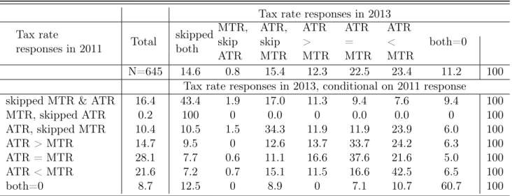
Table 1.3 presents the distribution of respondents’ answers across categories of average and marginal tax rates. The first three columns are the percent of respondents (of the subsample) who skipped both questions, the percent who only skipped the MTR question but answered the ATR question, and the percent who answered zero for both. The next three columns show the percent of respondents with survey MTR larger than, smaller than, and equal to ATR, conditional on answering both with at least one non-zero numbers. Around sixteen percent of respondents skipped both questions and another ten percent answered the question about ATR but not about MTR. Only one respondent skipped the question about the average tax rate and answered the question about their marginal tax rate.
Comparing average and marginal rates provides an indicator of whether respondents understand that in the progressive U.S tax system the average tax rate is always (weakly) less than the marginal tax rate. The relationship between MTR and ATR is due to the fact that (i.) statutory marginal tax rates increase with the level of taxable income, and (ii.) deductions and exemptions are always strictly positive. Whenever taxable income is positive, (ii.) implies that MTR is strictly greater than ATR. Only a third of responses are consistent with the progressive tax schedule (MTR>ATR). The largest percent of respondents gave the same number for both ATR and MTR, which was 29
percent of the sample, or 37 percent if I include those who reported zero for both.
Figure 1.1 displays a histogram of the survey measures of marginal and average tax rates in both waves of CogEcon. Reported marginal tax rates are in the top panel, while average tax rates are in the bottom panel. In both waves there are concentrated responses at 0, 15 and other statutory rates or round numbers. There is substantial heterogeneity in survey measures of average and marginal tax rates. In CogEcon 2011, roughly a quarter of responses were multiples of ten, around half were multiples of five.
Differences between the survey and computed rates is more informative. Figure 1.2 compares the mean survey and computed rates across values of total income. The top panel (Figure 1.2a) shows survey ATR larger than computed ATR across the income distribution. This pattern holds across both waves. The mean of the survey ATR tracks the mean of the computed ATR across the income distribution. The bottom panel (Figure 1.2b) compares survey and computed marginal tax rates across values of total income. The mean survey MTR tracking the mean computed MTR, with slight mean reversion, or the tendency to report rates closer to the mean tax rate in the population. People at low levels of total income overestimate their MTR relative to the computed rates, whereas people at higher incomes underestimate MTR. Again, this pattern holds across both waves.
The survey measures of tax rates provide information about income. To gain intuition, consider respondents answering completely randomly. The mean would be flat across the distribution of income because the survey measures would contain no information about income. Survey tax rates rise with income. After accounting for random noise, the distribution of survey measures might inform estimation of the distribution of income.
Figure 1.3 summarizes these differences between survey and computed rates. Each observation in 1.3a consists of a pair of ATR errors, which is the difference between survey and computed ATR, and 1.3b does the same but for MTR errors. The mass of observations in the first quadrant of Figure 1.3a means that respondents systematically report ATR larger than what is computed from their income. In contast, Figure 1.3b shows respondents scattered throughout all four quadrants, providing evidence of both heterogeneity in systematic errors, along with substantial randomness in the survey measures of marginal tax rates.
Looking at summary statistics in Table 1.4, there is substantial heterogeneity across respondents in the size of the difference between survey and computed tax rates (for both MTR and ATR). The survey minus computed difference for ATR is positive and significant (albeit heterogeneous). The survey minus computed difference for MTR is both positive (at low income) and negative (at high
income), but mostly not significantly different from zero. The survey minus computed pattern looks more similar for ATR than MTR.
1.3
Structural measurement model
The descriptive statistics provide compelling evidence of systematic differences between survey and computed tax rates, and substantial variation in the errors. For a given individual, differences between survey and computed tax rates could reflect systematic misperceptions, unobserved filing behavior, or survey noise. Survey responses were interpreted at face value, ignoring the fact that survey data is subject to misreporting or other errors with data handling, and that respondents do not always have information available when completing the survey. Income measurement error causes misclassification of marginal tax rates, and variation in the survey measures comes from systematic misperceptions and random noise. While it is unlikely that random noise in either variable could generate the systematic errors in the previous section, it could lead to erroneous inference about individual observations. Both would lead to inconsistent estimates of behavioral parameters.
I develop a statistical measurement model to combine information from survey and computed average and marginal tax rates. Survey responses about MTR, ATR and income (which is used to compute MTR and ATR) provide three indicators of latent taxable income. Separately identifying income and tax rate errors hinges on the known non-linear relationship between income and tax rates, and parametric assumptions about the (different) structure of the two errors. I estimate the error distribution for both survey tax rates and income. I then impute subjective and true rates while correcting for measurement error and systematic differences between the measures, and analyze heterogeneity in tax rate misperceptions.
My approach is similar to recent models in which the error structure of survey responses is compared to that from administrative data (Kapteyan and Ypma, 2007; Abowd and Stinson, 2013). Unlike these papers, my two measures are fundamentally different variables although they have a known functional relationship. My model uses information from MTR to detect income errors, which is conceptually similar to the approach of Sullivan (2009), who uses information from wages to detect misclassification of occupations. Both wages and occupations come from self-reported survey data.
to use discrete survey responses to estimate the distribution of a latent continuous variable when responses are subject to error. In KSS, the true underlying latent variable is continuous but the survey responses are discrete. In this application, the true marginal tax rate is a discrete variable, while responses are continuous.
1.3.1 Variables
Each individual i has survey measures of income, marginal tax rate and average tax rate across two waves of data (w = 1,2). Wave 1 refers to data collected in CogEcon 2011, with reference to tax year 2010. Wave 2 refers to data collected in CogEcon 2013, with reference to tax year 2012. The income, marginal tax rate and average tax rate variables that have the superscript ? are the unobserved true values. There is no superscript when the variable is observed in the data.
Income
• yi≡(yi,1, yi,2)0 is the vector of the log of reported income for individual i.
• y?i ≡y?i,1, yi,?2
0
is the vector of the log of true income for individual i. Marginal tax rates (MTR)
• mi≡(mi,1, mi,2)0 is the vector of reported marginal tax rates for individuali.
• m?i ≡m?i,1, m?i,20 is the vector of true statutory marginal tax rates for individuali. Average tax rates (ATR)
• ai ≡(ai,1, ai,2)0 is the vector of reported average tax rates for individuali.
• a?i ≡a?i,1, a?i,2
0
is the vector of true average tax rates for individuali.
1.3.2 Known income tax functions
1.3.2.1 Statutory relationship between income and MTR
Individuali’s true statutory marginal tax rate (m?i,w) in wavewis a function of true taxable income (I?
i,w), written as m?i,w = Mw
I? i,w
. Taxable income (I?
gross income (AGIi,w? ) minus deductions (Di,w? ), which is either the standard deduction or itemized deductions, and exemptions (E?i,w)
Ii,w? = maxAGIi,w? −Di,w? −Ei,w? ; 0 . (1.1) Adjusted gross income can also be written as the AGI share of total income (s?i,w) times total income:
AGIi,w? =s?i,w·Yi,w? . The marginal tax rate function Mw(·)is defined by tax law Mw Ii,w?
=τj ⇐⇒ Iwj−1 ≤Ii,w? < Iw j
(1.2)
and maps true taxable income into one of seven statutory tax rates, τj ∈ {0; 10; 15; 25; 28; 33; 35}.
The statutory marginal tax rate is τj when taxable income in wave w is between thresholds Iwj−1
and Iw j
. The top threshold for bracket j−1 is the bottom threshold for bracket j. These income thresholds depend on filing status (married or single), but subscripts for filing status are supressed to simplify notation. While the statutory rates are the same in 2010 and 2012, the functionMw(·)
changes because of adjustments to the taxable income thresholds.
1.3.2.2 Statutory relationship between income and tax liability Taxpayeri’s true tax liability in wavew,T?
i,w =Tw
I? i,w
, is a continuous, piece-wise linear deter-ministic function of taxable income
Tw Ii,w? =τj· Ii,w? −Iwj−1 +Cwj whenIwj−1 ≤Ii,w? < Iw j . (1.3)
That is, someone with taxable income betweenIwj−1 andIw j
is taxed at rateτj on all taxable income
above Iwj−1. Everyone with marginal tax rate τj (and the same filing status) pays tax Cwj on all
income less than threshold Ij−1, whereCj
w≡τ1·Iw1 +τ2· I2 w−Iw1 +...+τj−1· Iwj−1−Iwj−2 . By ignoring tax credits and assuming all income is taxed as wage or salary income, the tax liability computation is an upper bound on true tax liability at a given taxable income. This is because tax credits reduce tax liability and tax-preferred investments are taxed at lower rates than wages and salary income. Therefore, my estimate of the average tax rate errors, if anything, results in a lower bound on the ATR error.
1.3.3 Measurement equations
There are two definitions of income relevant to this analysis. Total income (Y) refers to money received from almost any source during the specified tax year. This corresponds to the definition of income that is observed in the data. Taxable income (I) is defined as total income minus all deductions, exemptions and adjustments.5
Survey measures of income are inherently noisy, and there has been an extensive literature on the causes and consequences of such errors.6 To account for measurement error in observed income, I follow the literature (e.g., Bound and Krueger (1991); Kapteyan and Ypma (2007)) and model observed log income asyi,w = logYi,w, equal to true log income (yi,w? ) plus random noise (ei,w)
yi,w =yi,w? +ei,w (1.4)
I assume true log income (y?i,w) across the two waves 1 and 2 has a bivariate normal distribution. I allow for wave-specific meanµy?
w and standard deviation σyw?, and correlation ρy? across the two
waves: y?i ≡ yi,?1, y?i,20 ∼BV Nµy? 1, µy2?, σ 2 y? 1, σ 2 y? 2, ρy ?
Measurement error is normally distributed random noise with mean zero, ei,w ∼ N 0, σe2
. Assuming the income error is unbiased is consistent with existing evidence from validation studies (Bound et. al (2001)). Assuming errors are mean zero with the same standard deviation (σe) in the
two waves, uncorrelated with true income and independent across waves, yields
Cov(y1, y2) =Cov(y1?+e1, y?2+e2) =Cov(y?1, y2?) =ρy?·σy?
1 ·σy?2 Hence, the joint distribution of observed income in waves 1 and 2 is
yi,1 yi,2 ∼N µy? 1 µy? 2 , σy2? 1 +σ 2 e ρy?·σy? 1 ·σy?2 ρy?·σy? 1 ·σy2? σ 2 y? 2 +σ 2 e
The three main assumptions are (i.) the functional form of the income distribution; (ii.) mea-5
More specifically, what I refer to as total income might typically be called gross income (GI). This includes money received from almost any source during the specified tax year and is the broadest income concept used for tax purposes. Adjusted Gross Income (AGI) equals gross income minus "above the line" deductions such as IRA contributions, student loan interest, and self-employed health insurance contributions. Taxable income equals AGI minus exemptions and deductions.
6
surement error is “classical”; (iii.) measurement error is independent across waves. In my main specification I make a fourth assumption, which is that the cross-wave correlation of true income (ρy?) is known (from another source).
The functional form seems reasonable given the likely sources of error in my data. Measurement error that is additive in logs is equivalent to having multiplicative error that follows a log-normal distribution. Respondents who answer the question with an exact amount often report rounded numbers (e.g., someone with income of 41,348 might say 40,000). Those who do not provide an exact amount are then prompted to select a range of income from a list of ranges. For these respondents we assign the midpoint but in fact all we know is that their income is within an interval of values; the intervals increase at higher levels of income, consistent with a lognormally distributed error term.
I also assume measurement error is “classical,” such that Covei,w, yi,w?
= 0. This assumption warrants discussion, as there is mixed evidence in previous studies about the reasonableness of this assumption. Bound and Krueger (1991), Bollinger (1998), Kapteyan and Ypma (2007), and Hudomiet (2013) all find evidence that reported income exhibits mean-reverting measurement error. People with low income overreport and those with higher income underreport. The implications of this assumption will be addressed when I interpret the results. However, Hudomiet (2013) finds that this is almost entirely at very low levels of income, and that there is no evidence of mean reversion for those with income above $10,000.
Finally, I assume that the income measurement error is uncorrelated across waves. By making this assumption I am attributing all systematic differences between the survey and computed tax rates to errors in tax rates. This assumption would be violated if respondents, for example, have private information about itemized deductions that is not captured in the CogEcon measures of income but impacts their tax rate responses.
1.3.3.1 Marginal and average tax rates
Taxpayeri’s reported marginal tax rate in wavew equals the true MTR plus an error term
where true MTR (m?i,w) is defined in the previous section. Taxpayer i’s reported average tax rate in wave wequals the true ATR plus systematic error and stochastic noise
ai,w =a?i,w+εai,w (1.6)
where true ATR is true tax liability (from previous section) divided by true adjusted gross income,
a?i,w = T
? i,w AGI? i,w
. The errors εai,w and εmi,w capture heterogeneity in survey reports, conditional on the true tax rates. If respondents had precise beliefs about their tax rates, then the errors εai,w and
εmi,w capture heterogeneity in misperceptions and random survey noise. If respondents do not have precise beliefs, then the reported values can be interpreted as an unbiased estimate of the mean subjective rates. Heterogeneity in survey measures includes systematic misperception, variation in reporting beliefs due to resolveable (but unresolved) uncertainty (on behalf of the respondent), and random survey noise.
There are a couple reasons why I choose to define true ATR with adjusted gross income (AGIi,w? ) in the denominator. First, this definition is often used by the IRS when analyzing average tax rates and by TurboTax when computing the average tax rate after filing one’s return. Respondents who recalled estimates of ATR from their tax software or tax professionals are likely reporting a noisy measure of average tax rate defined using AGI in the denominator. A more intuitive definition, and one more consistent with the wording of our survey question, uses a broader definition of income. As a robustness check I present estimates using true ATR defined as tax liability divided by total income,a?i,w= T
? i,w Y?
i,w
. This definition of true ATR is the preferred specification if respondents answer the question by dividing their perceived tax liability by perceived total income. As is expected, the mean bias in ATR is larger when using this broader measure of total income (Yi,w? ). The mean bias in perceived average tax rates is larger when using gross income or another measure with a broader tax base.
Modeling the marginal tax rate with additive error in the true rate could be contrasted with modeling the subjective rate in terms of the discrete statutory MTR. If people knew the tax table then I could model the tax response in terms of an underlying latent variable determining the categorical tax rate. However, only about half of respondents answer using one of the statutory marginal tax rates. Binning the tax responses ignores information contained in responses that are in between statutory tax rates. On the other hand, the presumed data generating process will not give the spikes in the data at the statutory marginal tax rates. Chapter 2 addresses this issue by
assuming respondents come from a mixture of two data generating processes. The first is with additive error, as in the model above, while the second assumes the subjective rate is a statutory MTR associated with subjective taxable income.
While respondents were asked for values between 0 and 100 in CogEcon 2011, they were not restricted like this in CogEcon 2013. Nevertheless, the distributions look similar in the two waves and the restricted domain in 2011 does not appear to have impacted responses. The functional form assumptions are used to tame the data and are not instrumental to interpreting the parameter estimates. Therefore, the baseline specification ignores censoring at 0 and 100. Moving forward it is important to better deal with cases of zero tax liability.
To close out the structural model I need to make distributional assumptions about MTR errors
εmi,w and ATR errors εai,w. Define the vector of tax rates responses as ri = (ai,mi)0 with ai =
(ai,1, ai,2) and mi = (mi,1, mi,2) as the vectors of ATR and MTR responses. I assume that the marginal and average tax rates, conditional on true income, have a multivariate normal distribution
ri|y?i ∼N(r?i +br,Σr)
over the average and marginal tax rate responses in both waves (four dimensional distribution). The vector br = (ba1, ba2, bm1, bm2)
0
captures mean biases in tax rate perceptions, where baw =
Eai,w−a?i,w and bmw = E mi,w−m?i,w
in each wave w, and
Σr= Σaa Σam Σma Σmm = σ2 a1 ρaσa1σa2 ρamσa1σm1 0 ρaσa1σa2 σ 2 a2 0 ρamσa2σm2 ρamσa1σm1 0 σ 2 m1 ρmσm1σm2 0 ρamσa2σm2 ρmσm1σm2 σ 2 m2
is the variance-covariance matrix. I letσaw represent the standard deviation of the ATR error (εaw)
in wavew, andσmw is the standard deviation of the MTR error (εmw) in wavew. The parameterρa= Corr(εa
1, εa2) is the correlation of ATR errors across waves, ρm = Corr(εm1 , εm2 ) is the correlation of MTR errors across waves, and ρam = Corr(εm1 , ε1a) = Corr(εm2 , εa2) is the correlation of ATR errors and MTR errors within the same wave. The values ofρa,ρm, andρam are between -1 and 1.
Correlation of ATR and MTR errors across different waves is set to zero: Corr(εm2 , εa1) = 0. In the baseline specification I assume the mean and variance are the same across waves, such thatba=baw
ATR and MTR errors are potentially correlated within the same wave, that ATR errors could be correlated across waves, MTR errors could be correlated across waves, but the ATR errors in one wave are uncorrelated with the MTR errors from the other wave.
1.3.4 Likelihood function
LetΩ denote the set of observed data, which is a vector Ωi = (yi,ri)0 of reported income and tax
rates for individuals i= 1, . . . , N. The likelihood L(θ|Ω) that the distributional parameters for the specified model are θgiven dataΩis proportional to the probabilityPr (Ωi|θ)of observingΩ
given the specified model and parametersθ:
L(θ|Ω)∝Pr (Ω|θ) =
N
Y
i=1
Pr (Ωi |θ) (1.7)
The log likelihood function for the model is then given by
LL (θ) =
N
X
i=1
ln{Pr (Ωi |θ)} (1.8)
Using Bayes law, the probabilityPr (Ωi |θ) equals the probability of reporting incomeyi times the
probability of reporting tax ratesri conditional on having reported income yi
Pr (Ωi |θ) = Pr (ri|yi, θ)·Pr (yi|θ) (1.9)
The term Pr (yi |θ) is simply the density f(yi|θ). To calculate Pr (ri|yi), I need to integrate
over the two-dimensional income measurement error distribution because latent true income is not observed in the data. Each realization of income measurement error vector e (conditional on observed incomeyi) pins down true incomeyi?, sincee=yi−y?i, which in determines true average
tax ratesa?i and marginal tax rates m?i.
Pr (ri |yi) = ˆ ˆ f(ri |ei,yi)·f(ei |yi) de = ˆ ˆ f(ri |y?i =yi−ei)·f(ei |yi) de
This integral forPr (ri|yi)does not have a simple closed-form representation due to the complicated
integrate over the reported tax rates. Therefore, the likelihood function does not have a tractable closed-form analytical expression.
I use Maximum Simulated Likelihood (MSL) to estimate the parameters of the model. The major complication in evaluating the likelihood function arises from the fact that true income is not observed. Estimating the parameters of the model by maximum likelihood involves integrating over the distribution of these unobserved income errors. This problem is solved by simulating the likelihood function. The simulated log-likelihood function is then given by
SLL (θ) =
N
X
i=1
ln ˇLi(θ) (1.10)
The contribution of each individualiisLˇi(θ), which is a simulated approximation toLi(θ), derived
as ˇ Li(θ) = 1 K K X k=1 Lki (θ) (1.11)
where the average is over the likelihood evaluated at each simulation draw
Lki (θ) = Pr ri|yi, ei(k)
·f(yi) (1.12)
and K is the number of pseudorandom draws of the vector of errors ei(k). The algorithm involves simulating a distribution of income errors for each respondent. The individual’s likelihood contri-bution is computed for each set of income errors, and density of the implied tax errors are averaged over the K values to obtain the simulated likelihood contribution.
1.3.5 Identification
Given my statistical model for observable data Ω given a parameter vector θ expressed via the probability functionPr (Ω|θ), the identification problem boils down to the following: do differences between survey and computed tax rates arise because of misperceptions or because measurement error in income induces errors in the computed rate?
The model is said to be theoretically point identifiable if there is a unique set of parameter estimates θ = (µy?, σy?, ρy?, σe, ba, bm, σa, σm, ρa, ρm, ρam) given the sample moments of the data.
The parameter vector includes three means, four standard deviations and four correlations. The sample moments include 3 means (3 in each wave), 3 standard deviations (3 in each wave). As for the correlations, within-wave there are 3 correlations.
Identification comes from having multiple indicators and repeated measures. Reported income, marginal tax rate and average tax rate provide three indicators of latent taxable income, and these variables are observed across two waves of data. Having a known functional relationship between true taxable income and true tax rates separately identifies the distribution of income measurement error and tax rate biases. Intuitively, identification can be broken into two steps, corresponding to parameters governing the income data generating process and parameters characterizing the tax rate errors.
The income parameters include those governing true income (µy?, σy? andρy?) and the standard
deviation of income measurement error (σe). When income measurement error is mean zero, the
mean of true log income (µy?) is identified by the mean of observed log income (µy), since µy? =
E (y?) =µy. Because measurement error in income is assumed to be uncorrelated with true income
and is uncorrelated across waves, two relationships hold:
1. σy2 =σ2y? +σ2e: variance of observed income is equal to the variance of true income plus the
variance of income measurement error. 2. ρy? =ρy· σ2 y?+σ 2 e σ2 y?
, which says that correlation of true income equals the correlation of observed income times one over the reliability ratio σ
2
y? σ2
y?+σ2e
.
Hence, once I identify the standard deviation of true income (σy?), the standard deviation of
in-come measurement error (σe) is identified by the standard deviation of observed income (σy). The
correlation of true income across waves (ρy?) is then pinned down by the correlation of observed
income (ρy). Alternatively, identifying the correlation of true income (ρy?) is enough to identify
the standard deviation of income measurement error (σe). Therefore, identification of σe requires
knowledge about the correlation of true income (ρy?) or the standard deviation of true income (σy?).
The tax rate error parameters ba, bm, σa, σm, ρa, ρm and ρam are identified once the income
parameters are known. The bias terms ba and bm are identified from the observed tax rates and
income, and mean zero income measurement error. This is a normalization to make errors have mean zero. The assumption that the tax rate errors are conditionally independent of income implies thatV ar(mi,w) =σ2m?+σm2, or that the variance of observed MTR is equal to the variance of true
MTR plus the variance of the MTR errors. The variance of true MTR (σm2?) is a deterministic
function of the true income distribution (characterized by µy? and σy?) and the known functional
Finally, identification of the correlation of ATR and MTR errors within wave (ρam), the
cor-relation of the ATR error across waves (ρa), and the correlation of MTR errors across waves (ρm)
exploits the known correlation of true income (ρy?) and the non-linear relationship between true
MTR and true ATR across the income distribution.
It is known that non-linear functions can greatly aid identification in measurement error models (Carroll et al., 2006, pp. 184). In this context, there are two non-linear relationships that facili-tate identification. First, as true income increases, both MTR and ATR increase, but at different rates. This creates variation in the difference between true MTR and true ATR. Another important mechanical source of identification comes from variability in how reliable reported income is de-pending on its location within tax bracket. When income falls toward the middle of a tax bracket, the true rate is known with greater likelihood than when income is close to a income cut-off of the tax bracket. I know the true MTR whenever adjusted gross income is measured without error and deductions perfectly observed. This helps separately identify the correlation of ATR and MTR errors within wave (ρam), the correlation of the ATR error across waves (ρa), and the correlation of
MTR errors across waves (ρm).
Therefore, identifying σe requires knowledge about the correlation of true income (ρy?) or the
standard deviation of true income (σy?). And knowing these three parameters is sufficient to identify
the tax rate error parameters σa, σm, ρa, ρm andρam.
The standard deviation of true income is also identified from the correlation of observed income and tax rates within waves. By assumption, the shared component of this correlation is due to true income. Combining income and tax rates helps identify the distribution of true income.
As described above, identification depends on a few important assumptions. First, tax errors are uncorrelated with true income and, therefore, uncorrelated with the true tax rate. Second, tax and income errors are uncorrelated. This assumption is critical, and relies on the fact that errors reflect random survey noise and systematic differences between perceived and true tax rates. If people who overreport income also overreport taxes then the pair of responses would appear consistent with one another and having a second measure is no longer helpful.
1.3.6 Estimation
Estimation of θ = (µy?, ba, bm, σy?, σe, σa, σm, ρa, ρm, ρam) is done using the method of maximum
simulated likelihood. In practice, I use between K= 50 and 200 draws per individual to simulate the likelihood in the baseline specification. Quasi-random Halton sequence draws, rather than random
draws, are used to simulate the likelihood because of the documented superior performance of quasi-random Halton draws in the simulation of integrals (e.g., Train 1999, Bhat 2001). Halton sequences are used to construct draws over the two-dimensional income measurement error. The individual’s likelihood contribution is computed for each set of income errors, and density of the implied tax errors are averaged over the K values to obtain the simulated likelihood contribution. A detailed description of the simulation algorithm and likelihood evaluation are in Appendix A.3.1.
In the main specification, I calibrate the correlation of true log income (ρy?) across years 2010
and 2012 to reduce computational issues associated with simulating the likelihood function. I set
ρy? = 0.9, which coincides with estimates of the second-year autocorrelation of log earnings from
other studies. Haider and Solon (2006) estimate an average first-order (one year) autocorrelation of 0.89 and average second-order autocorrelation of 0.82 using Social Security earnings data for a sample from the cohort born in 1931-1933 and studied between the ages of about 43 and 52. They show that the correlation for an alternative time frame, 1980-1991 rather than 1975-1984, results in slightly higher larger estimates, with first-order autocorrelation of 0.91 and second-order autocorrelation of 0.85. Parsons (1978) studies white male wage and salary earners and estimates the autocorrelation of earnings for different age categories (45-54 and 55-64) and three categories of educational achievement. For the 55-64 age category– the most relevant for CogEcon sample demographics–the first and second year autocorrelation are above 0.925 across education categories. and 0.970 for the lowest and highest education categories. The autocorrelation across years two and three is significantly different across the education groups, with autocorrelation of 0.674 for education=12, 0.863 for education=13-15 and 0.968 for education=16. The CogEcon sample of older and better educated workers suggests that 0.9 is a conservative estimate of the correlation of true income. However, the results are robust to both alternative assumptions about this correlation as well as estimating the correlation directly.
My optimization routine switches between the BHHH algorithm (for 5 iterations) and the BFGS algorithm (for 10 iterations) to compute the maximum likelihood estimate of parameters
(θ= (µy?, ba, bm, σy?, σe, σa, σm, ρa, ρm, ρam)). This includes three means, four standard deviations
and three correlations. Clustered robust standard errors are constructed from the asymptotically robust variance-covariance matrix using the outer product of the score to approximate the Hessian, clustering at the household level.
1.4
Parameter Estimates
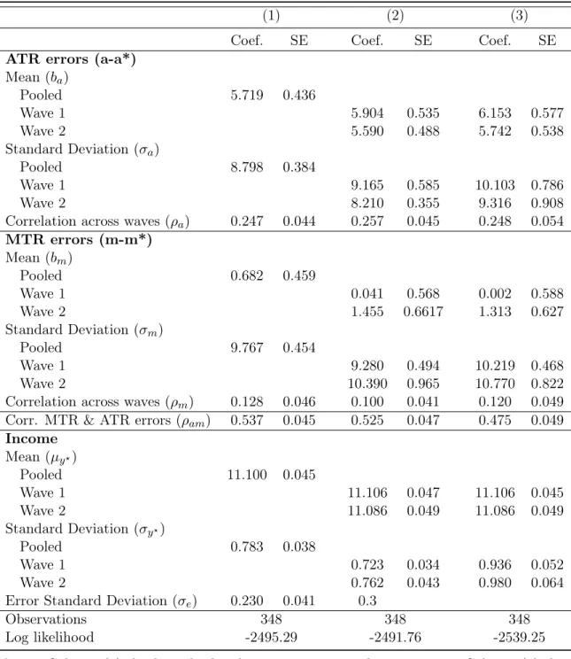
Table 1.5 presents the estimated structural parameter values (θ= (µy?, ba, bm, σy?, σe, σa, σm, ρa, ρm, ρam))
and standard errors for the full model of average tax rates, marginal tax rates and income (Equations 1.4, 1.5 and 1.6), and alternative specifications.
The first column of Table 1.5 reports the estimates for the full model. All of the parameters are estimated quite precisely. The mean of the ATR bias (ba) is almost 6 percentage points. A typical
person in CogEcon pays 11% of their income in federal income taxes, but perceives it as 17%. There is also substantial heterogeneity in these beliefs, as reflected by the distribution of errors around its mean value. The estimated standard deviation (σa) is8.8, meaning there is substantial unobserved
heterogeneity even accounting for measurement error in income. With the mean perceived rate of 17%, two standard deviations would go from around 0 to 30, which spans the range of true ATR that could reasonably be observed. Having the two waves of data allows me to estimate the correlation of ATR errors across years (ρa), which is estimated to be0.25.
The estimated parameters for the MTR errors show marked differences from the parameters for the ATR errors. There is no systematic difference between the survey and true marginal tax rates, as the mean of the MTR bias (bm) is statistically indistinguishable from zero. The estimated standard
deviation (σm) is9.8, which is over one percentage point larger than the standard deviation of the
ATR errors. Finally, the estimated correlation of MTR errors across years (ρm) is around 0.13,
which is smaller in magnitude than the correlation of ATR errors but still significantly different from zero.
Estimates of the standard deviation of the ATR errors (σa) and MTR errors (σm) are
econom-ically large and significant. Heterogeneity in reported rates comes from unexplained variation in systematic errors, yet also reflects various measurement problems. In terms of the reported tax rates, there are both small scale errors such as approximating, guessing the truth, rounding despite being well-informed, and larger random noise. The positive correlation suggests that the large vari-ation is not simply a failure to properly measure perceptions of tax rates. For example, a person who has a large itemized deduction could have lower taxable income and lower MTR and ATR than is account for in the model.
These correlations of the MTR errors across waves and ATR errors across waves are small compared to the within-year correlation of MTR and ATR errors (ρam) of over 0.5, which is both
overestimate their MTR. However, I cannot rule out the possibility that the positive correlation is the result of having accurate measures of the survey tax rates and errors in the computed rates. Regardless of the interpretation, the large positive estimate of ρam provides strong evidence that
tax rate errors are not purely random noise.
Though not my primary focus, the estimated parameters on the income distribution are in-teresting in their own right, as this is the first paper to identify income measurement error from reported tax rates. True log income yi? has an estimated mean of 11.1, corresponding to median income $66,171. The standard deviation of true log income is bσy? = 0.78 , the standard
devia-tion of income measurement error of bσe = 0.23. These estimates imply a reliability ratio of 0.92,
which is defined as the (estimated) variance of the latent true income divided by the variance of the noisy measure.7 Reliability ratios provide a way to compare the extent of measurement error across studies, wherein a higher reliability measure is associated with less survey noise. This estimate is slightly higher than what is typically found in validation studies of income. Bound and Krueger (1991) find slightly higher reliability of CPS earnings, in the low0.80 and0.90 ranges for men and women, respectively. In contrast, Duncan and Hill (1985) estimate a ratio of 0.76when comparing reported earnings from employees at a particular company with the company’s payroll records.
1.4.1 Specification checks and further analyses
These estimated parameters from the full model of ATR, MTR and income are robust to alternative specifications. First, columns (2) and (3) of Table 1.5 present estimated parameters of a two-equation model of ATR and income (Equations 1.4 and 1.6) and a two-equation model of MTR and income (Equations 1.4 and 1.5), respectively. The estimates are similar to those in the full model, but with larger standard errors. There are also some noticeable differences between the estimates. The correlation of ATR errors across waves (ρa) and MTR errors across waves (ρm) are twice as large,
and the standard deviation of the ATR error (σa) is slightly larger (bσa= 9.758versusσba= 8.798). It
is important to note that I estimate the two-equation model of MTR and income without simulating the likelihood function because I do not need to integrate out the income measurement error. The consistency of the estimates across models provides important evidence that the simulated likelihood estimation stategy is not impacting the results. Details about constructing the likelihood functions
7 b σ2 y? b σ2 e+bσ 2 y? = (0.78)2 (0.23)2+ (0.78)2 = 0.92
and estimating the parameters of these models are provided in Appendix C.
Column (4) in 1.5 presents estimates of the full model (Equations 1.4, 1.5 and 1.6) but assuming the MTR and ATR errors are uncorrelated (ρam = 0). As expected, the estimated correlation of
ATR errors across waves (ρa) is similar to in a model of only ATR and income, and the estimated
correlation of MTR errors across waves (ρm) is similar to what it is when estimated in a model of
only MTR and income. Marginal and average tax rates are mechanically linked, so it’s important to estimate the equations jointly to account for their dependence. Once ATR errors are included in the model the correlation of the MTR errors across waves is close to zero. These correlations highlight the importance of jointly modeling ATR and MTR.
Column (5) in Table 1.5 presents estimates for the two-equation MTR model (Equations 1.4 and 1.5) when relaxing the assumption that the correlation of true income is ρy? = 0.9. The estimate
of this correlation is slightly larger, ρby? = 0.91, but the assumed value is well within the 95%
confidence interval for the estimated correlation. Under reasonable assumptions about the cross-wave correlation of true income, I get estimates of the income measurement error that are similar to what I find using marginal tax rate responses and are consistent with what has been previously found in the literature. Since my goal is to account for measurement error in income when comparing reported tax rates with measures computed using reported income, the exact estimate of income measurement error is of lesser importance. These results suggest that assuming ρy? = 0.9 is a
reasonable assumption in this context.
This exercise also provides indirect evidence that simulating the likelihood function for the full three-equation model in fact limits what I can identify using my current set of numerical routines. As discussed in Appendix C, estimation of the three equation model introduces computation issues that make it sometimes difficult to determine convergence. It raises questions about identification of the model. However, the results from this exercise provide suggestive evidence that estimation problems are computational in nature and are stemming from simulating the likelihood function rather than problems with identification.
Parameter estimates are generally robust to varying assumptions about the correlation of true income. A large correlation of true income is needed to justify the substantial variation in tax perceptions conditional on reported income. This is because the a higher correlation of income means that variation in the observed values gets attributed to measurement error rather than variation in income. The higher the correlation of true income, the larger the estimate of the income measurement error. Intuitively, if the true income is highly correlated across waves then
variation in observed income across waves must be explained by random noise (measurement error) because true income acts as a fixed component and does not vary much.
Table 1.6 presents the estimated structural parameter values and standard errors when allowing the mean and standard deviation of true income and tax perceptions to differ across waves. Column (1) is repeated from Table 1.5 for reference. In column (2), the distribution of true income and the tax rate errors can be different across waves. The estimation routine appears unstable, so I calibrate the income measurement error atσe= 0.3. The same patterns show up in the individual waves and
the estimated parameters when pooling the observations across waves is in between the estimated parameters for the individual waves. While the standard deviation of ATR errors and MTR errors are both around 9.5 percentage points in 2010, but diverge in 2012. In particular, the standard deviation of the ATR errors falls from 9.3 to 8.3 percentage points, while the standard deviation of the MTR errors increases from 9.5 to 10.5 percentage points the standard deviations diverge in 2012. The mean ATR error hardly changes, while the mean MTR error increases from−0.01to 1.5. These changes are noteworthy in light of differences in the question wording across waves.
Ignoring survey response error overstates the heterogeneity in tax beliefs. Column (3) imposes the restriction that income is measured without error (σe = 0). Comparing columns (2) and (3)
shows how income measurement error affects other estimated parameters. As noted, this induces downward bias in the estimated mean error in tax beliefs. When incorporating income measurement error there appears to be a significant decline in the standard deviation of the tax rate errors. Without accounting for measurement error in income, the standard deviation of the difference between survey and reported rates hover around 10 percentage points, the exact value depending on the wave and whether it is ATR or MTR. These standard deviations are reduced to around 9 percentage points once accounting for measurement error, which is approximately 1 percentage point smaller, or 10 percent of the overall variation. But the decline is not economically significant, as the magnitude of these declines is miniscule compared to the overall level of these rates. While the fully structural model requires strong assumptions, it allows me to rigorously account for income measurement error and establish that the descriptive patterns cannot be explained by errors in the computed rates. This modest impact of income measurement error reinforces the conclusion that there are systematic biases and substantial heterogeneity in perceptions of tax rates.
1.5
Systematic heterogeneity in tax perceptions
In this section I relax the assumption that tax rate biases are constant across individuals and explore how the misperceptions vary with observable characteristics. I focus on how the systematic errors are related to demographic characteristics, cognitive ability, general financial sophistication and the use of paid tax preparers.8 To motivate this analysis, consider Figures 1.4 and 1.5. Figure 1.4 compares the distribution of tax rate errors for respondents in the bottom and top quarters of cognitive ability (number series score) and Figure 1.5 compares the distribution of tax rate errors for respondents who used paid tax preparers and those who did not. The graphs are of the kernel density estimates of the difference between reported rates and the imputed true rates. Imputations come from the conditional expectations md?i,w = Eb
h m?i,w |θ,b Ωi,w i and ad?i,w = Eb h a?i,w |θ,b Ωi,w i , which will be described more fully in Section 1.6. Respondents in the bottom quarter of cognitive ability (number series score) display much greater variation in their errors than