Discussion paper
SAM 7 2010
ISSN: 0804-6824 FEBRUARY 2010
INSTITUTT FOR SAMFUNNSØKONOMI
DEPARTMENT OF ECONOMICS
Optimal Redistributive Taxation with both
Extensive and Intensive Responses
BY
LAURENCE JACQUET, ETIENNE LEHMANN,
AND
BRUNO VAN DER LINDEN
Optimal Redistributive Taxation with both Extensive and
Intensive Responses
Laurence JACQUETy
Norvegian School of Economics and Business Administration, CESifo and IRES - Université Catholique de Louvain
Etienne LEHMANNz
CREST, IRES - Université Catholique de Louvain, IZA and IDEP
Bruno VAN DER LINDENx IRES - Université Catholique de Louvain, FNRS, ERMES - Université Paris 2 and IZA
January 28, 2010
Abstract
This paper characterizes the optimal income taxation when individuals respond along both the intensive and extensive margins. Individuals are heterogeneous in two dimensions: their skills and their disutility of participation. Preferences over consumption and work e¤ort can di¤er with the skill level, only the Spence-Mirrlees condition being imposed. We derive an optimal tax formula thanks to a tax perturbation approach. This formula generalizes previous results by allowing for income e¤ects and extensive margin responses. We provide a su¢ cient condition for optimal marginal tax rates to be nonnegative everywhere. The relevance of this condition is discussed with analytical examples and numerical simulations on U.S. data.
JEL Classi…cation: H21, H23.
Keywords: Optimal Tax formula, Tax perturbation, Random participation.
We thank for their comments participants at seminars at GREQAM-IDEP in Marseilles, IAP CORE/Ghent/KULeuven seminar in Ghent, CREST, NHH, Uppsala, Louis-André Gerard-Varet meeting in Mar-seilles, NTNU in Trondheim, the CESifo Norwegian-German seminar on public Economics with a particular mention to Sören Blomquist, Pierre Cahuc, Nicolas Gravel, Bas Jacobs, Guy Laroque, Patrick Pintus, Ray Rees, Emmanuel Saez, Agnar Sandmo, Fred Schroyen, Laurent Simula and Alain Trannoy. Any errors are ours. Lau-rence Jacquet would like to thank Skipsreder J.R. Olsen og hustrus legat to NHH. This research has been funded by the Belgian Program on Interuniversity Poles of Attraction (P6/07 Economic Policy and Finance in the Global Economy: Equilibrium Analysis and Social Evaluation) initiated by the Belgian State, Prime Minister’s O¢ ce, Science Policy Programming.
yAddress: Norwegian School of Economics and Business Administration (NHH), Economics Department, Helleveien 30, 5045 Bergen, Norway. Email: [email protected]
zAddress: CREST-INSEE, Timbre J360, 15 boulevard Gabriel Péri, 92245, Malako¤ Cedex, France. Email: [email protected].
xAddress: IRES - Département d’économie, Université Catholique de Louvain, Place Montesquieu 3, B1348, Louvain-la-Neuve, Belgium. Email: [email protected]
I
Introduction
This paper provides an optimal nonlinear income tax formula that solves the redistribution problem when individuals respond along both the intensive (in-work e¤ort) and extensive (par-ticipation) margins. For that purpose, we consider an economy where individuals are hetero-geneously endowed with two unobserved characteristics: their skill level and their disutility of participation. Because of the …rst heterogeneity, employed workers typically choose di¤erent earnings levels. Because of the second heterogeneity, at any skill level, only some individuals choose to work. The government can only condition taxation on endogenous earnings and not on the exogenous characteristics whose heterogeneity in the population are at the origin of the redistribution problem.1 Therefore, positive marginal tax rates are necessary to transfer income from rich to poor individuals, while inherently distorting intensive labor supply decisions. More-over, when individuals of a given skill level experience a rise either in the tax level they paid when employed or in the bene…t for the nonemployed, some of them leave the labor force. This rise of the so-called participation tax2 thereby generate distortions along the extensive margin of the labor supply.
Since Mirrlees (1971), the optimal tax problem is usually solved by searching for the best incentive-compatible allocation and applying variational calculus condition to these allocations. While this method has been proved successful, it lacks economic intuitions. We instead derive the optimal tax formula by measuring the e¤ects of a change in marginal tax rates on a small interval of income levels.3 This “tax perturbation approach” emphasizes the economic mechanisms at work but faces the following di¢ culty: because of the nonlinearity of the tax schedule, when an individual responds to a tax perturbation by a change in her labor supply, the induced change of her gross income a¤ects in turn the marginal tax rate she faces, thereby inducing a further labor supply response. To take this “circular process” into account, we de…ne behavioral elasticities along the optimal nonlinear tax schedule. Thanks to this rede…nition, we can intuitively express optimal marginal rates as a function of the social welfare weights, the skill distribution and the behavioral elasticities. This formula generalizes previous results by allowing for income e¤ects and extensive margin responses.
We also provide a su¢ cient condition under which optimal marginal tax rates are nonneg-ative. Clarifying the restrictions that ensure this result is an issue in the optimal income tax
1Because the second heterogeneity matters only for the participation decisions, the government faces a
multi-dimensional screening problem that is reduced to the “random participation” model introduced by Rochet and Stole (2002).
2
Which equals the tax level plus the bene…t for the non-employed, so that each additional worker increases the governments’revenue by the level of the participation tax.
3
We verify in Appendix that the solution derived thanks to the tax perturbation approach is consistent with the Mirrleesian approach in terms of incentive-compatible allocations.
literature with only intensive responses.4 Intuitively, the optimality of nonnegative marginal
tax rates holds whenever social welfare weights are decreasing along the skill distribution, so the distortion induced by positive marginal tax rates are compensated by the equity gain of transferring income from high to low-skilled workers. Adding an extensive margin response, we …nd a condition on the ratio one minus the social welfare weights over the extensive be-havioral response. Strikingly, the optimal participation tax equals this ratio when individuals respond only along the extensive margin. When both margins are included, we show show that optimal marginal tax rates are nonnegative whenever this ratio decreases along the skill distri-bution. While our su¢ cient condition is expressed in terms of endogenous variables, we discuss its relevance in practice and give examples of speci…cations on primitives where this condition holds. For instance, when the government has a Maximin objective, we argue that the additional restrictions are fairly weak.
Using U.S. data, we also calibrate the model to illustrate the quantitative implications of our optimal tax formula. These simulations suggest that the introduction of an extensive margin reduces marginal tax rates by a signi…cant amount, while the tax schedule remains qualitatively similar. In our sensitivity analysis, marginal tax rates are always positive. However, for the least skilled workers, participation taxes are typically negative under a Benthamite criterion, while they are always positive under Maximin. The literature on optimal taxation in the pure extensive model has typically found these results and interprets optimality of negative participation tax at the bottom of the skill distribution as a case for an Earned Income Tax Credit (EITC) form of income-tax transfer instead of a Negative Income Tax (NIT) form (see Saez 2002). We provide examples with a strictly positive lower bound for the earnings distribution,5 a negative participation tax at this minimum (as for the EITC) and nonnegative marginal tax rates above this minimum (as for the NIT).
Our paper contributes to the literature that aims at making the literature on optimal income taxation useful for applied thinking in public …nance. For many years after the seminal paper of Mirrlees (1971), the numerous developments of the theory focused on useful technical re…nements but provided little economic intuitions. A …rst important progress was made when, in the absence of income e¤ects, Atkinson (1990), Piketty (1997) and Diamond (1998) re-expressed optimality conditions derived from the Mirrlees model in terms of behavioral elasticities. Saez (2001) made a second important step forward by deriving an optimal tax formula thanks to a tax perturbation approach.6 He takes into account the abovementioned “circular process” by
4
See e.g. Mirrlees (1971), Sadka (1976), Seade (1982), Werning (2000) or Hellwig (2007), or the counterexam-ples given by Choné and Laroque (2009b).
5
We assume a strictly positive minimum for the skill distribution.
6Christiansen (1981) introduces the tax perturbation approach. However, he did not derive any implication for
the optimal income tax, his focus being on the optimal provision of public goods and the structure of commodity taxation. Revecz (1989) proposes a method to derive an optimal income tax formula in terms of elasticities but
expressing his optimal tax formula in terms of the unappealing notion of “virtual”7 earnings
distribution and veri…es the consistency of his solution to the Mirrlees one. He furthermore allows for income e¤ects. We avoid the use of virtual densities thanks to our rede…nition of behavioral elasticities.
The aforementioned papers neglect labor supply responses along the extensive margin, while the empirical labor supply literature emphasizes that labor supply responses along the extensive margin are much more important (see e.g. Heckman 1993). Saez (2002) derives an optimal tax formula in an economy with both intensive and extensive margins. For that purpose, he develops a model where agents can choose among a …nite set of occupations, each of them being associated to an exogenous level of earnings. However, he has no analytical result for the mixed case where both the extensive and intensive margins matter. Moreover, he focuses essentially on the EITC/NIT debate about whether working poor should receive more transfers than non-employed individuals, while we discuss the conditions under which marginal tax rates should be nonnegative. In addition, our formula allows for income e¤ects.8 Finally, our treatment of the intensive margin is more standard and it allows considering a continuous earnings distribution. This seems to us more appropriate for studying marginal tax rates than the discrete occupation setting of Saez (2002).9
The paper is organized as follows. The model is presented in Section II. Section III derives the optimal tax formula in terms of behavioral elasticities thanks to a tax perturbation method. This section also compares this tax formula to the literature. Section IV provides a condition su¢ cient to get optimal nonnegative marginal tax rates and examples where this condition is satis…ed. Section V presents simulations for the U.S. In appendix, we develop the formal model. In particular, we solve it for the optimal allocations thanks to the usual optimal control approach. We verify that this solution is consistent with the one we derive in the main text.
does not consider the abovementioned circular process. Hence his solution is not consistent with the Mirrlees one (see Revecz 2003 and Saez 2003). Using a tax perturbation method, Piketty (1997) derives the optimal nonlinear income tax schedule under Maximin. He too neglects to take into account the circular process but this has no consequence since he assumes away income e¤ects. Roberts (2000) derives it also under Benthamite preferences.
7
Saez (2001, p.215) de…nes the virtual density at earnings levelzas “the density of incomes that would take place atz if the tax scheduleT(:)were replaced by the linear tax schedule tangent toT(:)at levelz”.
8The formal model in the Appendix of Saez (2002) allows for the possibility of income e¤ects. Moreover, the
appendix of the NBER version of Saez (2002) extends his optimal tax formula with both extensive and intensive responses to the case of a continuum of earnings but without income e¤ects.
9
Boone and Bovenberg (2004) introduce search decisions in the Mirrlees model. This additional margin has a similar ‡avor as a participation decision. However, their speci…cation of the search technology implies that any individual with a skill level above (below) an endogenous threshold searches at the maximum intensity (does not search).
II
The model
II.1 Individuals
Each individual derives utility from consumption C and disutility from labor supply or e¤ort
L. More e¤ort implies higher earnings Y, the relationship between the two depending also on the individual’s skill endowment w. The literature typically assumes that Y = w L. To avoid this unnecessary restriction on the technology, we express individuals’ preference in terms of the observables (C and Y) and the individuals’ exogenous characteristics (including
w). This in addition enables us to consider cases where the preferences over consumptionC and e¤ort L are skill-dependent. Skill endowments are exogenous, heterogeneous and unobserved by the government. Hence, consumption C is related to earnings Y through the tax function
C=Y T(Y).
The empirical literature has emphasized that a signi…cant part of labor supply responses to tax reforms are concentrated along the extensive margin. We integrate this feature by considering a speci…c disutility of participation which makes a di¤erence in the level of utility only between
workers (for whom Y > 0) and nonemployed (for whom Y = 0). This disutility may be due to commuting, searching for a job, or a reduced amount of time available for home production. However, for some people, employment has a value per se. Some of them would feel stigmatized if they had no job. Let denote an individual’s disutility of participation net of this stigma, if any. We assume that people are endowed with di¤erent (net) disutility of participation . As for the skill endowment, is exogenous and the government cannot observe it. Because of this additional heterogeneity, individuals with the same skill level may take di¤erent participation decisions. This is consistent with the observation that in all OECD countries, skill-speci…c employment rates always lie inside(0;1).
For tractability, we need that labor supply decisions Y among employed workers depend only on their skill and not on their net disutility of participation. To get this simpli…cation, we need to impose some separability in individuals’preferences. We specify the utility function of an individual of type (w; ) as:
U(C; Y; w) IY >0 (1)
whereIY >0 is an indicator variable equal to one if the individual works and zero otherwise. The
gross utility function U(:; :; :) is twice-continuously di¤erentiable and is concave with respect to (C; Y). Individuals derive utility from consumption C and disutility from labor supply, so UC0 >0>UY0 . Last, we impose the strict-single crossing (Spence-Mirrlees) condition. We assume that, starting from any positive level of consumption and earnings, more skilled workers need to be compensated by a smaller increase in their consumption to accept a unit rise in their earnings. This implies that the marginal rate of substitution U0
skill level. Hence we have:
UY w00 (C; Y; w) UC0 (C; Y; w) UCw00 (C; Y; w) UY0 (C; Y; w)>0 (2)
The distribution of skills is described by the density f(:), which is continuous and positive over the support [w0; w1], with 0 < w0 < w1 +1. The lowest skill being nonzero, we leave aside the issue of redistribution where some people have a severe handicap. The size of the total population is normalized to 1 so Rw0w1f(w)dw = 1. The distribution of conditional on skill levelw is described by the conditional densityk(:; w) and the cumulative distributionK(:; w), with k( ; w) def @K( ; w)=@ . The density is continuously di¤erentiable. It is worth noting that w and may be distributed independently or may be correlated. The support of the distribution is ( 1; max], with max +1. The assumption about the lower bound is made for tractability since it ensures a positive mass of employed workers at each skill level.
Each agent solves the following maximization problem max
Y U(Y T(Y); Y; w) IY >0
where the choice of Y can be decomposed into a participation decision (i.e. Y = 0 orY > 0) and an intensive choice whenY >0 (i.e. the value ofY). For a worker of type(w; ), choosing a positive earnings levelY to maximizeU(C; Y; w)subject to C =Y T(Y) amounts to solve
Uw
def max
Y U(Y T(Y); Y; w) (3)
In particular, two workers of the same skill levels but with di¤erent disutilities of participation face the same intensive choice program, thereby taking the same decisions along the intensive margin.10 LetY
w be the intensive choice of a worker of skill wand letCw be the corresponding consumption level, soCw =Yw T(Yw). The gross utility of workers of skill wtherefore equals
Uw =U(Cw; Yw; w). We ignore the nonnegativity constraint on Yw when solving the intensive choice program. We verify in our simulations that the minimum of the earnings distribution is always positive (since we assumew0 >0). So, we are right to neglect the possibility of bunching due to the nonnegativity constraint.
1 0
The key assumption for this result is that preferences over consumption and earnings for employed agents vary only with skills and do not depend on the net disutility of participation . Such property is obtained under weakly separable preferences of the form
W(C; Y; w; ) = V(U(C; Y; w); w; )
U0(C; w; ) if
Y >0
Y = 0
whereW is discontinuous at Y = 0. V(:; :; :) is an aggregator that is increasing in its …rst argument. Function
U(:; :; :)veri…es UC0 >0>UY0 and (2). U 0
(:; :; :)describes the preference of the nonemployed and increases in its …rst argument. FunctionsU(:; :; :),U0(:; :; :)and V(:; :; :) are twice-continuously di¤erentiable over respectively
R+ R+ [w0; w1],R+ [w0; w1] R+ andR [w0; w1] R+. Finally, we assume that for given levels ofC,Y,
wand b, the function 7!V (U(C; Y; w); w; ) U0(b; w; )is decreasing and tends to+
1whenever tends to the lowest bound of its support. All results derived in this paper can be obtained under this more general speci…cation, the additional di¢ culty being only notational
We now turn to the participation decisions. Letb= T(0)denote the consumption level for individuals out of the labor force. We call bthe welfare bene…t. If an individual of type (w; ) chooses to work, she gets utilityUw . If she chooses not to participate she obtains U(b;0; w). An individual of type (w; ) chooses to work if Uw U(b;0; w) , Uw U(b;0; w). Therefore, the density of workers of skillw is given by h(w)de…ned as:
h(w)defK(Uw U(b;0; w); w) f(w) (4)
with some abuse of notation since h(w) does not make explicit the dependence of h(:) with respect toband toUw. The functionh(w)is twice-continuously di¤erentiable, increasing inUw and decreasing in b, with respective derivativesh0U(w) andh0b(w). The cumulative distribution isH(w) =Rw0w h(n) dn. There are H(w1) employed workers and 1 H(w1) nonemployed.
II.2 Behavioral elasticities
We de…ne the behavioral elasticities from the intensive choice program (3) and the extensive margin decision (4). When the tax function is di¤erentiable, the …rst-order condition associated to the intensive choice (3) implies:
1 T0(Yw) = U 0 Y UC0
(5) where the derivatives ofU(:)are evaluated at(Cw; Yw; w). When, in addition, the tax function is twice di¤erentiable, the second-order condition writes:11
UY Y00 2 U 0 Y U0 C UCY00 + U 0 Y U0 C 2 UCC00 T00(Yw) UC0 0 (6) Whenever the second-order condition (6) holds strictly, which we henceforth assume through the rest of this section, the …rst-order condition (5) de…nes implicitly12 earningsY
w as a function of skill level and of the tax function. The elasticity w of earnings with respect to the skill level equals:13 w def w Yw _ Yw = w Yw [U 00 Y w UC0 UCw00 UY0 ] U00 Y Y 2 U0 Y U0 c U 00 CY + U0 Y U0 c 2 U00 CC T00(Yw) UC0 UC0 (7) 1 1
By the concavity of U(:; :; :) on (C; Y), the second-order condition is satis…ed if the tax schedule is locally linear or convex (so thatT00(:) 0), or is not “too concave”.
1 2
In addition, one has to assume that among the possible multiple local maxima ofY 7!U(Y T(Y); Y; w), a single one corresponds to the global maximum. If program Y 7! U(Y T(Y); Y; w ) admits two global maxima for a skill levelw , workers of a skill levelwslightly above (below)w would strictly prefer the higher (lower) maximum due to the strict single-crossing condition (see Equation (2)). Hence, functionw7!Ywexhibits a discontinuity at skill w . Moreover, again by the the strict single-crossing condition, function w 7! Yw is nondecreasing. So, it is discontinuous on a set of skill levels that is at worst countable (and at best empty), which is of zero measure.
1 3
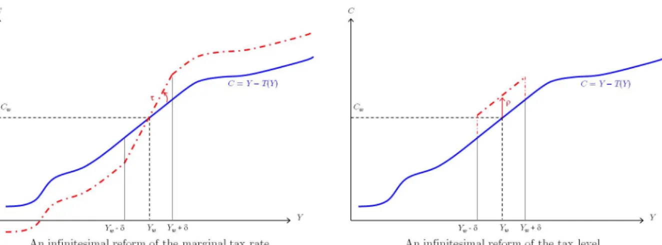
Figure 1: Tax reforms around Yw de…ning behavioral responses "w and w.
Leth^(Y) andH^ (Y) denote respectively the density and cumulative of the earnings distrib-ution among employed workers, with@H^(Y)=@Y = ^h(Y). Therefore, one has for all skill levels thatH^(Yw) H(w). From Equation (7),h(w) andbh(Yw) are related by:
Yw
w w ^h(Yw) h(w) (8)
If the left-hand side of (6) is nil, then the functionY 7! U(Y T(Y); Y; w)becomes typically constant aroundw. Therefore, individuals of typeware indi¤erent between a range of earnings level, so the functionn7!Ynbecomes discontinuous at skilln=w. The same phenomenon also occurs when the tax function is downward discontinuous atYw (T00(Y) tends to minus in…nity, so (6) is violated). Conversely, bunching of types occurs when w = 0 (i.e. T00(Y) tends to plus in…nity). This corresponds to a kink of the tax function. From now, we assume T(:) is di¤erentiable. Hence we rule out bunching. However, this assumption is relaxed in appendix where we solve the model in terms of incentive-compatible allocations and study what happens when bunching occurs.
We now consider di¤erent elementary tax reforms and compute how they a¤ect the intensive (3) and extensive choices (4). The …rst elementary tax reform captures the substitution e¤ect around the actual tax schedule. The marginal tax rateT0(Y)is decreased by an amount over the range of earnings [Yw ; Yw+ ]. So doing, the level of tax at earnings level Yw is kept constant, and so is Cw. The reform is illustrated in the left part of Figure 1.
compen-sated elasticity of earnings with respect to1 T0(Y):14 "w def 1 T0(Yw) Yw @Y @ = UY0 Yw UY Y00 2 U0 Y Uc0 UCY00 + U0 Y Uc0 2 U00 CC T00(Yw) UC0 >0 (9)
When the marginal tax rate is decreased by , a unit rise Yw in earnings generates a higher gain Cw = (1 T0(Yw) + ) Yw of consumption. Therefore, the workers substitute earnings for lower leisure. Finally, this reform only has a second-order e¤ect on Uw, thereby on the participation decisions.15
The next elementary tax reform captures the income e¤ect around the actual tax schedule. The level of tax is decreased by a lump sum amount over a range of earnings[Yw ; Yw+ ]. This reform is illustrated in the right part of Figure 1. Along the intensive margin, the behavioral response for a worker of skill wto this reform is captured by the income e¤ect:
w def @Y @ = U0 Y U0 C U 00 CC UCY00 U00 Y Y 2 U0 Y Uc0 UCY00 + U0 Y Uc0 2 U00 CC T00(Yw) UC0 (10)
This term can be either positive or negative. However, when leisure is a normal good, the numerator is positive, hence the income e¤ect (10) is negative.
The " -reform" illustrated in the right part of Figure 1 also induces some individuals of skill
w to enter the labor market. We capture this extensive response for individuals of skillw by:
w def 1 h(w) @h(w) @ = h0 U(w) h(w) U 0 C (11)
which stands for the percentage of variation in the number of workers with a skill level w. Finally, we measure the elasticity of participation when, together with a uniform decrease of the tax level by , the welfare bene…t b rises by (i.e. when T(Y) +b is kept constant). This reform captures income e¤ects along the extensive margin. The (endogenous) semi-elasticity of the number of employed workers of skillw with respect to such a reform equals:
w def h0U(w) h(w) U 0 C(Cw; Yw; w) + h0b(w) h(w) = w+ h0b(w) h(w) (12)
The behavioral responses given in (7), (9), (10), (11) and (12) are endogenous. They depend on skill levelw, earnings levelY and the tax functionT(:). In particular, the various responses along the intensive margin given in (7), (9) and (10) are standard (see e.g. Saez (2001)), except for the presence of T00(:) in their denominators. An exogenous increase in either w, , or
1 4The elasticity"
w is calledcompensated since the tax level is kept unchanged at earnings levelYw.
1 5
Decreasing T0(:) by implies a rise Yw of earnings, which itself increases Cw by Cw =
(1 T0(Y
w) + ) Yw. Therefore the impact on Uw is given by Uw = U(Cw; Yw; w) =
[(1 T0(Yw) + )UC0 +UY0] Yw =UC0 ("wYw=(1 T0(Yw))) 2 where the second equality follows (5) and (9)
induces a direct change in earnings 1Yw. However, this change in turn modi…es the marginal tax rate by 1T0 = T00(Yw) 1Yw, inducing a second change in earnings 2Yw. Therefore, a “circular process” takes place: The earnings level determines the marginal tax rate through the tax function and the marginal tax rate a¤ects the earnings level through the substitution e¤ect. The term T00(Yw) UC0 captures the indirect e¤ects due to this circular process (in the words of Saez (2001), see also Saez (2003) p. 483 and Appendix A). Unlike Saez (2001), we do not de…ne the behavioral responses along an hypothetical linear tax function, but along the actual (or later optimal) tax schedule, that we allow to be nonlinear. Therefore, our behavioral responses’parameters (7), (9) and (10) take into account the circular process and exhibit a term
T00(:) in their denominator.
II.3 The Government
The government’s budget constraint takes the form
b=
Z w1 w0
(T(Yw) +b) h(w) dw E (13) whereE is an exogenous amount of public expenditures. For each additional worker of skill w, the government collects taxesT(Yw) and saves the welfare bene…tb.
Turning now to the government’s objective, we adopt a welfarist criterion that sums over all types of individuals a transformationG(v; w; )of individuals’utilityv, with G(:; :; :) twice-continuously di¤erentiable and G0v > 0. Given the labor supply decisions, the government’s objective writes = Z w1 w0 (Z Uw U(b;0;w) 1 G(Uw ; w; ) k( ; w)d (14) + Z max Uw U(b;0;w) G(U(b;0; ); w; ) k( ; w)d ) f(w)dw
Redistribution is ensured by assumingG00vv <0orG00vw<0, the latter meaning that the objective function compensates agents endowed with lower skills.
Let denote the marginal social cost of the public fundsE. For a given tax functionT(:),we denote gw (respectively g0) the (average and endogenous) marginal social weight associated to employed workers of skill w(to the nonemployed), expressed in terms of public funds by:
gw def E G 0 v(Uw ; w; ) UC0 (Cw; Yw; w) jw; Uw U(b;0; w) (15) g0 def E G 0 v(U(b;0; w); w; ) UC0 (b;0; w) j > Uw U(b;0; w) (16)
The government values an additional dollar to the h(w) employed workers of skill w (to the 1 H(w1)nonemployed) asgwtimesh(w)dollars (g0times1 H(w1)dollars). The government
wishes to transfer income from individuals whose social weight is below 1 to those for which the social weight is above 1. As will be clear below, g0 and the shape of the marginal social weightsw7!gw entirely summarize how the government’s preferences in‡uence the optimal tax policy. The only properties we have is that g0 and gw are positive. In particular, the shape of
w7!gw can be non-monotonic, decreasing or increasing and we can have g0 above or belowgw0. However, a government that has redistributive concerns would typically exhibits a decreasing shapew7!gw of social welfare weights, as it will be discussed in Section IV.
III
Optimal marginal tax rates
III.1 Derivation of the optimal marginal tax formula
The government’s problem consists in …nding a nonlinear income tax scheduleT(:) and welfare bene…tbto maximize the social objective (14), subject to the budget constraint (13) and to the labor supply decisions along both margins. In this section we directly derive the optimal tax formula through a small perturbation of the optimal tax function. Following Mirrlees (1971), Appendix B solves the government’s problem in terms of incentive-compatible allocations, using optimal control techniques and veri…es that both methods lead to the same optimal tax formulae:
Proposition 1 The optimal tax policy has to verify T0(Yw) 1 T0(Yw) =A(w) B(w) C(w) (17) 0 =C(w0) (18) 1 g0 1 Z w1 w0 h(n) dn Z w1 w0 gn h(n) dn= (19) Z w1 w0 n T0(Yn) + n (T(Yn) +b) h(n)dw where A(w)def w "w B (w)def H(w1) H(w) w h(w) C(w)def Rw1 w f1 gn n T0(Yn) n(T(Yn) +b)g h(n) dn H(w1) H(w)
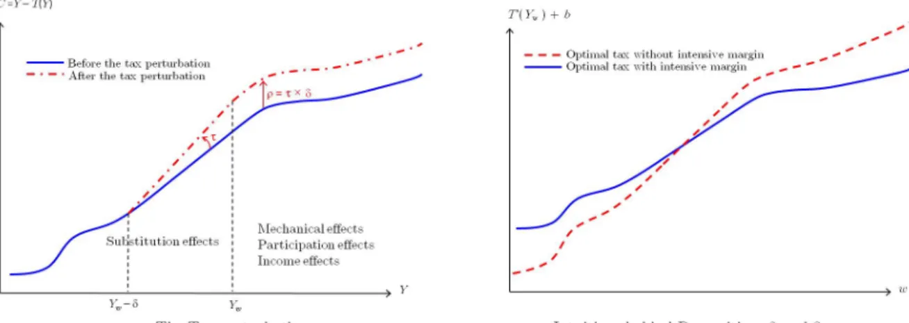
Equation (17) summarizes the trade-o¤ behind the choice of the marginal tax rate at earnings level Yw. We consider the e¤ects of the in…nitesimal perturbation of the tax function depicted in the left part of Figure 2. Marginal tax rates are uniformly decreased by an amount over a range of earnings[Yw ; Yw]. Therefore, the tax levels are uniformly decreased by an amount = for all skill levelsnabovew. This tax reform has four e¤ects: asubstitution e¤ect for tax payers whose earnings before the reform are in [Yw ; Yw], and some mechanical, income and participation response e¤ects for tax payers with skill nabovew.
Figure 2: The optimal tax schedule
Substitution e¤ect The substitution e¤ect takes place on the range of gross earnings[Yw ; Yw]. The mass of workers a¤ected by the substitution e¤ect is^h(Yw) . For these workers, according to Equation (9), the decrease by of the marginal tax rate induces a rise Yw of their earnings, with
Yw =
"w Yw 1 T0(Yw)
The tax reform has only second-order e¤ect onUw, thereby on the participation decisions and on their contribution to the government objective. However, the rise in their earnings increases the government’s tax receipt byT0(Yw) Yw. Hence, given that = , the total substitution e¤ect equals
Sw=
T0(Yw)
1 T0(Yw) "w Yw ^h(Yw) (20)
Workers of skill n above w face a reduction in their tax level without change in their marginal tax rate. This has three consequences.
Mechanical e¤ects First, absent any behavioral response for these workers, the government gets units of tax receipts less from each of the h(n) workers of skill n. However, the tax reduction induces a higher consumption levelCn, which is valued gnby the government. Hence the total mechanical e¤ect at skill wis:
Mw=
Z w1 w
(1 gn) h(n) dn (21)
Income e¤ects Second, the tax reduction induces each of the workers of skill n to change their intensive choice by Yn= n (see Equation (10)). This income response has only a …rst-order e¤ect on the government’s budget: each of theh(n) workers of skill npaysT0(Yn) Yn
additional tax. Hence, the total income e¤ect at skilln equals: Iw =
Z w1
w n
T0(Yn) h(n) dn (22)
Participation e¤ects Finally, the reduction in tax levels induces n h(n) individuals of skillnto enter employment (see Equation (11)). The change in participation decisions has only a …rst-order e¤ect on the government’s budget. Each additional worker of skill n pays T(n) taxes and the government saves the welfare bene…t b. Hence, the total participation e¤ect at skillw equals:
Pw =
Z w1 w
n (T(Yn) +b) h(n) dn (23) The sum of Sw, Mw, Iw and Pw should be zero if the original tax function is optimal. Rearranging terms then gives
T0(Yw) 1 T0(Yw) = 1 "w Rw1 w f1 gn n T0(Yn) n(T(Yn) +b)g h(n) dn Yw ^h(Yw) (24) which gives (17) thanks to (8).
Equation (18) describes the e¤ects of giving a uniform transfer to all employed workers. This tax pertubation does not a¤ect marginal tax rates, so it only induces mechanical, income and participation e¤ects. The sum of (21), (22) and (23) evaluated for w=w0 should be nil at the optimum, which leads to (18). Equations (17) and (18) implie that optimal marginal tax rate are nil at the minimum earnings level.16
To grasp the intuition behind Equation (19), consider a unit increase in welfare bene…t b
and a unit lump-sum decrease in the tax function for all skill levels. This reform does neither change marginal nor participation tax rates. Hence, it has only mechanical and income e¤ects along the intensive and extensive margins. This reform induces a (mechanical) loss of the tax revenues valued 1 by the government and a gain in the social objective. The latter amounts to g0 1
Rw1
w0 h(n) dn for nonemployed people and to
Rw1
w0 gn h(n) dn for the employed workers. Therefore, the mechanical e¤ect corresponds to the left-hand side of (19). The right-hand side captures the income e¤ects along both margins.17 First, through the income response along the intensive margin, earnings change by Yn = n. This a¤ects tax revenues by the weighted integral of Yn T0(Yn) = n T0(Yn). Second, participation decisions change through the income e¤ect by h(n) = n h(n). Since for each additional worker of skilln, tax revenues
1 6Intuitively, increasing the marginal tax rate at a skill levelw0 improves equity when the extra tax revenue can be redistributed towards a positive mass of people with skills equal or lower tow0. Since the mass of agents with skillw0 is nil, a positive marginal tax rate atw0 does not improve equity. It does however distort the labor
supply. The optimal marginal tax rate at the lowest skill level then equals zero (Seade (1977)).
1 7
Diamond (1975), Sandmo (1998) and Jacobs (2009) emphasize that the social value of public funds should only take into account behavioral responses due to income e¤ects. Equation (19) shows that only income e¤ects along the intensive w and extensive w margins matter.
increase byT(Yn) +b, the total impact is the weighted integral of n (T(Yn) +b). When leisure is a normal good, one has n<0and n<0. Therefore, sinceT(Yn) +bis typically positive for most workers, we expect that larger income e¤ects along both margins increase the aggregate average of social welfare weights (g0 and gn’s) above1.
III.2 Comparison with the optimal tax literature
Equation (17) decomposes the determinants of the optimal marginal tax rates into three com-ponents. A(w) is the e¢ ciency term. B(w) captures the role of the skill distribution among employed individuals. Finally, C(w) stands for the social preferences for income redistribution, taking into account the induced responses through income e¤ects and along the participation margin.
There are two apparent di¤erences between our formulation of the e¢ ciency term A(w) and the literature. The …rst is the presence ofT00(Yw) in the de…nitions (7) and (9) of w and
"w. This is due to our de…nitions of behavioral responses along a potentially nonlinear income
tax schedule and the induced endogeneity of marginal tax rates. However, in the ratio w="w, these additional terms cancel out. So, the termA(w) is the same whether we de…ne behavioral elasticities w and"w along the optimal tax schedule (as we do in the present paper) or along a “virtual” linear tax schedule (as usually done in the literature, see e.g. Piketty 1997, Diamond 1998 and Saez 2001). The second di¤erence is induced by our assumption on preferences (1). The literature is typically restricted to the case where preferences over consumption and work e¤ort do not vary with skill levels, and are described by U(C; Y =w). Then, it happens that the numerator of A(w) coincides with one plus the uncompensated elasticity of the labor supply. This is counterintuitive, since it suggests thatceteris paribus marginal tax rates increases with the latter elasticity. Our more general assumption on preferences enables us to stress that in fact, what matters is the elasticity w of earnings with respect to skill levels. Marginal tax rates are then inversely related to the compensated elasticity in the vein of the “inversed elasticity” rule of Ramsey.
The termB(w)captures the role of theskill distribution. Consider an increase of the marginal tax rate around the earnings levelYw (the left part of Figure 2). The induced distortions along the intensive margin are larger, the higher is the skillwtimes the number of workers at that skill level,w h(w)(Atkinson 1990). However, the gain in tax revenues is proportional to the number
H(w1) H(w) of employed workers of skillnabovew. Two di¤erences with the literature are worth noting. First, because of the extensive margin responses, what matters is the distribution of skills among employed workers, and not within the entire population. Since h(w)=f(w) equals the employment rate of workers of skillw and(H(w1) H(w))=(1 F(w))equals the aggregate employment rate above skill w, one can further decompose B(w) into its exogenous
and endogenous components through: B(w) = 1 F(w) w f(w) H(w1) H(w) 1 F(w) h(w) f(w)
The …rst term on the right-hand side equals the exogenous skill distribution term of Diamond (1998).18 Second, the distribution term in (Saez 2001, Equation (19)) concerns the (virtual) distribution of earnings and not the skill distribution. This was the way for him to get rid of the counterintuitive presence of the uncompensated labor supply elasticity in the numerator of his e¢ ciency term. Using (7), one then gets that wB(w) = H^(Yw1) H^(Yw) =Yw ^h(Yw), so our optimal tax formula can also be expressed in terms of the earnings distribution, as we did in (24). Both formulations have their advantage. On the one hand, the earnings distribution has the advantage to be directly observable. On the other hand, it is easier to index individuals by their exogenous skill rather than their endogenous earnings. We therefore choose to present the two formulations, letting the reader choosing which of the two she/he prefers.
The term C(w)captures the in‡uence ofsocial preferences for income redistribution, taking into account the induced responses through income e¤ects and along the participation margin. It equals the average of mechanical, income and participation e¤ects for all workers of skill n
above w. Diamond (1998) considers the case where participation is exogenous and there is no income e¤ect.19 Introducing income e¤ects or participation responses in the analysis amounts
to modifying the social weight to
gn
def
gn+ n (T(Yn) +b) + n T0(Yn)
Saez (2002, p. 1055) has explained why the government is more willing to transfer income to groups of employed workers for which the participation response n or the participation tax
T(Yn)+bis larger. The behavioral parameter nis positive, so a decrease in the level of tax paid by workers of skilln induces more of them to work. Whenever the participation taxT(Yn) +b is positive, tax revenues increase, which is bene…cial. We argue that a similar interpretation can be made for the income e¤ect. Typically, leisure is a normal good (hence n <0). Then, a decrease in the level of tax paid by workers of skill n induces them to work less through the income e¤ect. Whenever they face a positive marginal tax rate, this response decreases the tax they pay, which is detrimental to the government. Therefore, the government is more willing to transfer income to groups of employed workers for which income e¤ects are lower (i.e. higher
n) and marginal tax rates are lower (Saez 2001).
1 8Diamond (1998)’s
C(w)corresponds to ourB(w)and vice-versa.
1 9
Under redistributive preferences, marginal social weightsgw are decreasing in skill levelsw. Then,C(w) is increasing, but remains below 1. When in addition preferences are maximin (see Atkinson 1975, Piketty 1997, Salanié 2005, Boadway and Jacquet 2008 among others), then the marginal social weights for workersgware nil, soC(w)is constant and equals1.
IV
Properties of the second-best optimum
IV.1 Su¢ cient condition for nonnegative marginal tax rates
We …rst consider the special case where labor supply decisions take place only along the extensive margin, as assumed in Diamond (1980) and Choné and Laroque (2005, 2009a), so"w = w= 0. The optimal tax formula then veri…es:20
T(Yw) =
1 gw w
b (25)
The optimal level of taxes then trades o¤ the mechanical e¤ect (captured by the social weight
gw) and the participation response e¤ect (captured by the participation response w) of a rise in the level of tax. Marginal tax rates are then everywhere nonnegative if along the optimal allocation, the function Y 7! (1 gw)= w is increasing. The following Proposition shows that this result remains valid in the presence of responses along the intensive margin.
Proposition 2 If along the optimal allocation, w 7! 1 gw
w is increasing, marginal tax rates
are always nonnegative. Furthermore, they are almost everywhere positive, except at the two extremities Yw0 and Yw1.
This Proposition is proved in Appendix C. The intuition is illustrated in the right part of Figure 2. This …gure depicts the level of taxT(Yw) paid by a worker of skillw, as a function of her skill level. When labor supply responses are only along the extensive margin, the optimal tax schedule is represented by the dashed curve. It corresponds to the optimal trade-o¤ between mechanical and participation e¤ects. Under the Assumption w 7! (1 gw)= w is increasing in w, this function is increasing in the skill level. However, when the worker can also decide along her intensive margin, such an increasing tax function and its positive marginal tax rates induce distortions of the intensive choices. Hence, the optimal tax function, which is depicted by the solid curve, is ‡atter than the optimal curve without intensive margin to limit the distortions along the intensive margin. It also has to be as close as possible to the optimal curve without intensive margin to limit departures from the optimal trade-o¤ between participation and mechanical e¤ects.
Proposition 3 If along the optimal allocation, w7! 1 gw
w is increasing in w and if gw 1 for
all skill levels, then in work bene…ts (if any) are smaller than the welfare bene…t b.
The assumption thatgw 1for all skills is restrictive. It implies that the optimal tax in the case without intensive responses is characterized by leaving to the least skilled workers lower
2 0In the absence of response along the intensive margin, substitution e¤ects
Sw in (20) and income e¤ects Iw in (22) are nil at each skill level. Therefore, the sum of mechanicalMw and participationPw e¤ects have to be nil at each skill level, which gives (25).
bene…t than to the nonemployed (hence a Negative Income Tax is optimal). This result remains valid in the presence of intensive responses since the optimal tax function under unobserved skills is ‡atter than the one under observed skills. Proposition 3 emphasizes this result.
In the absence of behavioral responses along the intensive margin, in-work bene…ts for the working poor (of skill w0) are larger than welfare bene…ts if and only ifgw0 >1. By continuity, as long as the compensated elasticity (along the intensive margin) "w0 is small enough, in-work bene…ts should remain higher than welfare bene…ts hence an EITC is optimal. This has already been emphasized by Saez (2002).
IV.2 Examples
The su¢ cient condition in Propositions 2 and 3 depends on the patterns of social weights gw and extensive behavioral response w which are endogenous. This subsection provides examples of speci…cations of the primitives where the su¢ cient conditions in Propositions 2 and 3 are satis…ed.
Our …rst example speci…es the primitives of the model in such a way thatgw and w become exogenous. For this purpose, individuals’preferences are quasilinear: U(C; Y; w) =C V(Y; w) withV0
Y;VY Y00 >0>VY w00 . The marginal utility of consumptionUC0 (C; Y; w)is then always equal to one. Second, we specify the distribution of disutility of participation conditional on skill levelwto beK( ; w) = exp (aw+ ), whereaw is a skill-speci…c parameter adjusted to keep some individuals out-of-the labor force at the optimum. Then w is always equal to parameter according to Equation (11) and is thereby constant along the skill distribution. Finally, the social objective is linear in utilities with skill-speci…c weights w. Since the speci…cation of individuals’utility rules out income e¤ects, we have thatgw= w=
Rw1
w0 wdw (see (15), (16) and (19)). Therefore, under redistributive social preferences, w7! w is decreasing, so (1 gw)= w is decreasing. Marginal Tax rates are then nonnegative according to Proposition 2. Note that in such case, one must havegw0 >1, so this speci…cation does not rule out a negative participation tax to be optimal for working poor.
This …rst example is however very speci…c. In general, we think it is very plausible that
w 7! 1 gw is non-increasing and w 7! w is strictly decreasing. First, a redistributive gov-ernment typically gives a higher social welfare weight on the consumption of the least skilled workers. Second, there is some empirical evidence that the elasticity of participation, which equals (Yw T(Yw) b) w is typically a nonincreasing function (see e.g. Juhn et alii 1991, Immervoll et alii 2007 or Meghir and Phillips 2008). Since consumption Yw T(Yw) is an increasing function, one can expect w to decrease along the skill distribution.
Assume that the utility function is additively-separable, i.e.
U(C; Y; w) =u(C) V(Y; w) (26)
with u0C;VY0 ;VY Y00 > 0 > u00CC;VY w00 . The additive separability restriction is only made for
technical convenience. However showing within the pure intensive model that marginal tax rates are positive without imposing the additive separability assumption (26) was a real issue (see e.g. Sadka 1976, Seade 1982, Werning 2000). We add another restriction on preferences. For an employed worker, a given earnings level is obtained thanks to lower e¤ort, the more skilled the worker is. However, for a nonemployed, no e¤ort is supplied hence a larger skill does not improve utility. Hence we assume:
Vw0 (Y; w)
<
= 0 if Y
>
= 0 (27)
So, the skill-speci…c threshold Uw U(b;0; w) of is constrained to be an increasing function of the skill level. The following properties are shown in Appendix E.
Property 1 IfK( ; w)is strictly log-concave wrt to ,w7!k( ; w)=K( ; w)is non-increasing in w and (26)-(27) hold, then w7! w is strictly decreasing.
The logconcavity of K(:; w) is property veri…ed by most distributions commonly used. It is equivalent to assuming that k( ; w)=K( ; w) is decreasing in . That k( ; w)=K( ; w) is non-increasing inwencompasses the speci…c case wherewand are independently distributed.
Property 2 If either Maximin social preferences or Benthamite social preferences and (26)-(27), then w7!gw is non-increasing
Maximin (i.e. maximizingu(b)) and Benthamite (i.e. G(Uw ; w; ) =Uw ) social pref-erences are polar speci…cations. Combining Properties 1 and 2, the relation w7! (1 gw)= w is increasing provided that gw remains below1. Therefore, Propositions 2 and 3 hold under the Maximin, utility functions verifying (26) and (27), K( ; w) strictly log-concave wrt to and
k( ; w)=K( ; w) nonincreasing in w. Moreover, if the government is instead Benthamite and ifgw0 1, then Propositions 2 and 3 are again ensured.
V
Numerical simulations for the U.S.
This section implements our optimal tax formula with real data to analyze if and to what extent optimal schedules resemble real-world schedules and if not, how to reform them. This exercise also allows checking whether our su¢ cient condition for non-negative marginal tax rates is empirically reasonable.
V.1 Calibration
To calibrate the model we need to specify social and individual preferences and the distribution of characteristics(w; ). We consider Benthamite and Maximin social preferences. We choose a speci…cation of individual preferences that enables us to control behavioral responses along the intensive margin. Following Diamond (1998), we assume away income e¤ects along the intensive margin (hence w 0) and assume the compensated elasticities to be constantly equal to "
along a linear tax schedule. Moreover, individuals’preferences are concave so that a Benthamite government has a preference to transfer income from high to low income earners. Hence, we specify U(C; Y; w) = C Yw 1+ 1 " + 1 1 1
The parameter " corresponds to the compensated elasticity along a linear tax schedule (see Equation (9)) while parameter drives the redistributive preferences of a Benthamite govern-ment. Saezet al. (2009) surveys the recent literature that estimates the elasticity of earnings to marginal tax rates. They conclude that “The most reliable longer-run estimates range from0:12 to 0:4” in the U.S. We take a central value of " = 0:25 for our benchmark. For the concavity of preferences, we take = 0:8 in the benchmark case. We conduct sensitivity analysis with respect to these two parameters.
To calibrate the skill distribution, we take the earnings distribution from the Current Popu-lation Survey for May 2007. We use the …rst-order condition (5) of the intensive program to infer the skill level from each observation of earnings. We consider only single individuals to avoid the complexity of interrelated labor supply decisions within families. Using OECD tax database, the real tax schedule of singles without dependent children is well approximated by a linear tax function at rate27:9%and an intercept at$ 4024:9on an annual basis.21 We use a quadratic kernel with a bandwidth of $3822 to smooth h(w). High-income earners are underrepresented in the CPS. Diamond (1998) and Saez (2001) argue that the skill distribution actually exhibits a fat upper-tail in the US, which has dramatic consequence for the shape of optimal marginal tax rates. We therefore expand (in a continuously di¤erentiable way) our kernel estimation by taking a Pareto distribution, with an index22 a = 2 for skill levels between w = $20374 and
w1= $40748.23 This represents only the top3:1%of our approximation of the skill distribution. One …nally needs to calibrate the conditional distribution of . For numerical convenience, we choose a logistic and skill-speci…c speci…cation of the form
K( ; w) = exp ( aw+ w ) 1 + exp ( aw+ w )
2 1
We multiply by52the weakly earnings given by the CPS survey.
2 2
An (untruncated) Pareto distribution with Pareto indexa >1is such that Pr(w >wb) =C=wbawitha; C 2R+0.
2 3
Parameters aw and w are calibrated to obtain empirically plausible skill-speci…c employment rates, denoted by Lw, and elasticities of employment rates with respect to the di¤erence in disposable incomes Cw b, denoted w. We take
Lw = 0:7 + 0:1 w w0 w1 w0 1=3 w = 0 1 w w0 w1 w0 with 0= 0:5 and 1= 0:1 These speci…cations are consistent with the empirical fact that the employment rateLw is larger for high-skilled than for low-skilled. The average employment rate in the current economy equals 75:3%. The elasticity w is equal to 0:45 on average. Unreported simulations point out that the properties of the optimal tax schedule are robust to changes in the parameters of the above
w!Lw relationship. A sensitivity analysis will illustrate how the calibration of w modi…es the optimal tax pro…le.
We take b= $2381since the net replacement ratio for a long term unemployed worker whose previous earnings equals67%of average wage equals9%in 2007 according to OECD. Given this calibration of the current economy, we …nd that the buget constraint (13) is veri…ed only when we set the exogenous revenue requirement toE = $6110per capita.
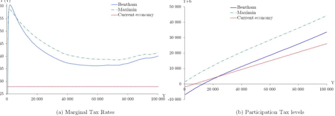
V.2 Benchmark simulations
Figure 3 plots the optimal marginal tax rates (Panel (a)) and participation tax levels (Panel (b)) as functions of earnings, under the Benthamite (solid line) and Maximin (dotted line) criteria. We focus on earnings below $100;000.24 Consistent with Proposition 2, marginal tax rates are always positive, under both criteria. Moreover, there is no distortion at the very bottom of the earnings distribution whose value is Yw0 = $508. This contrasts with the positive marginal tax rate obtained under Maximin, in a model with intensive margin only. In this case, everyone in the objective function is atY =Yw0, so the equity e¤ect is positive and therefore,T0 Yw0 >0 at the Maximin optimum (Boadway and Jacquet 2008). When both extensive and intensive margins are modeled, there is only a positive mass of welfare weight on the nonemployed, under Maximin. Then, a positive marginal tax rate on the least-skilled workers would create a distortion without bringing any equity gain hence T0 Y
w0 = 0. Panel (a) illustrates that this result of no distortion is very local: When Y = $2;150, the marginal tax rate climbs to 60:5% (58:8%) under Benthamite (Maximin) preferences. Beyond, marginal tax rates follow the usual U-shaped pro…le (Salanié 2003), under both objective functions. Under Maximin, marginal tax rates are higher than under Bentham, except at the bottom end (forY lower thanY = 5;900$). Remarkably, optimal marginal tax rates are signi…cantly higher than the current 27:9%, except for the very low end of the earnings distribution. This is valid under both objectives.
2 4
Income earners above $100;000 correspond to 4:65%, 3:73% and 5:66% of the population at the current economy, the Benthamite optimum and the Maximin optimum, respectively.
Figure 3(b) illustrates that participation tax levels at the bottom of the earnings distribution are typically negative under a Benthamite criterion. The optimality of a negative participation tax on the poorest workers is usually interpreted as a case for an Earned Income Tax Credit (EITC) (Saez 2002). We …ndb= $2;665and T(Yw0) = $9;345. Contrastingly, Figure 3(b) also emphasizes that participation tax levels at the bottom of the earnings distribution are positive, under Maximin. A Negative Income Tax (NIT) then prevails. This is a standard result of the pure extensive margin model (Choné Laroque 2005) which is still valid here when considering both extensive and intensive margins together.25 Intuitively, it is hardly desirable to transfer income to the least skilled workers, since their well-being does not matter under Maximin. At the Maximin optimum, we …ndb= $4;190and T(Yw0) = $3;860.
Figure 3: The simulation under the benchmark calibration
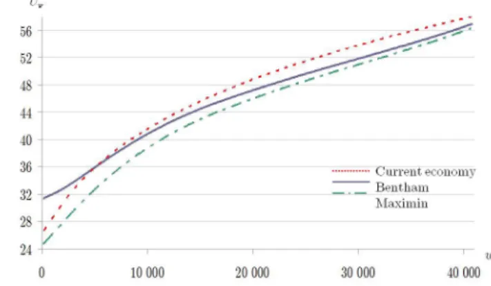
Figure 4(a) describes how the negative participation tax on least skilled workers enables to boost employment rates well above their values in the current economy. Moreover, Panel (b) illustrates how these negative participation tax rates (in the Bentham economy) increase the utility levels of low-skilled workers signi…cantly beyond their values in the current economy.
V.3 Sensitivity analysis
All our various sensitivity analysis exercises point out that the U-shape pro…le is valid and none of them displays negative marginal tax rates. The only con…guration where our su¢ cient condition for nonnegative marginal tax rate is violated requires an extremely low . And, even then, the marginal tax rates are still positive. This section therefore focuses on the quantitative implications of parameters on the optimal tax rates.
As illustrated in Figure 5(a), the levels of marginal tax rates are quite sensitive to the
Figure 4: Optimal allocations
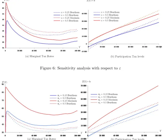
Figure 5: Sensitivity analysis with respect to
parameter of the individual preferences. Any rise of increases the marginal tax pro…le by a substantial amount since the planner becomes more averse to inequality. The participation tax levels increase (decrease) with below (above) Y around$20;000. Higher redistributive tastes increase the transfers towards the low-paid workers and the other workers pay more taxes (see Panel (b)).
Figure 6(a) illustrates that marginal tax rates decrease with the elasticity of earnings ", as theoretically expected from the implied decrease of A(w) in Equation (17). Figure 6(a) illustrates this result with"equals to0:25and0:5, under Maximin and Benthamite preferences.26
Figure 6(b) emphasizes that participation taxes decrease (increase) with " for earnings above (below) roughly around$30;000, under both criteria.
2 6
Figure 6: Sensitivity analysis with respect to"
Figure 7: A lowerw7! w in the calibration of the current economy
The next exercise studies the impact of reducing the participation response w. Figure 7 plots the tax schedule when the parameter 0 shrinks from 0:5 to 0:1. This reduction of the elasticities of employment rates w7! w (hence the reduction of w) signi…cantly increases the marginal tax rates (see Panel (a)), as expected from the implied decrease of C(w) in Equation (17). Moreover, as also expected from theory, the participation tax levels increase (Panel (b)). This exercise highlights the quantitative implications of introducing the extensive margin.
Another sensitivity exercise considers a more decreasing w 7! w in the current economy hence a more decreasing w 7! w. Figure 8 plots the tax rates when ( 0; 1) (0:75;0:25) (solid curves) instead of ( 0; 1) (0:5;0:1)(dashed curves). As expected from the C(w) term in Equation (17), the marginal tax rates then increase. Also, the participation tax curves become more increasing, under both criteria (Pannel (b)), as expected from theory.
Figure 8: A more decreasingw7! w in the current economy
Our calibration abstracts from income e¤ects. For consistency with the theoretical frame-work, we also focus on single households and then abstract from the interactions between labor supply decisions within couples. However, those dimensions are not necessary to show how crucial it is to consider both labor supply margins to give tax policy recommendations.
VI
Conclusion
This paper explored the optimal income tax schedule when labor supply is simultaneously along both the extensive and the intensive margins. Individuals are heterogeneous in two dimensions: their skills and their disutility of participation. We derived a fairly mild su¢ cient condition for nonnegative marginal tax rates over the entire skill distribution. This condition is derived thanks to a new method to sign distortions (along the intensive margin) in screening models with random participation. Our exercise illustrated that negative participation tax rates can optimally coexist with positive marginal tax rates everywhere.
Using U.S. data, we implemented our optimal tax formula. This exercise emphasized that the U-shaped optimal tax schedule found in the model with intensive margin only is still valid when both labor supply margins are considered. But introducing the extensive margin quite substantially reduces the marginal tax rates. Interestingly, the marginal tax rates are always positive in our simulations.
This paper also points to extensions. The method to sign distortion along the intensive margin can been applied to other contexts of nonlinear pricing theory where agents are charac-terized by a multi-dimensional parameter that is unobserved by the principal. It would also be interesting to extend the numerical simulations to data sets from other countries.
Appendices
A
Behavioral Elasticities
We de…ne
Y(Y; w; ; )def 1 T0(Y) + UC0 (Y T(Y) + (Y Yw) + ; Y; w)
+UY0 (Y T(Y) + (Y Yw) + ; Y; w)
The …rst-order condition (5) is equivalent toY(Yw; w;0;0) = 0. WhenT(:)is twice-di¤erentiable, one has (using (5)):
YY0 (Yw; w;0;0) = UY Y00 2 U 0 Y U0 c UCY00 + U 0 Y U0 c 2 UCC00 T00(Yw) UC0 (28a) Yw0 (Yw; w;0;0) = 1 T0 UCw00 +UY w00 = U00 Y w UC0 UCw00 UY0 UC0 (28b) Y0 (Yw; w;0;0) = UC0 (28c) Y0 (Yw; w;0;0) = 1 T0 UCC00 +UCY00 = U 00 CY UC0 UCC00 UY0 U0 C (28d) The second-order condition writes YY0 (Yw; w;0;0) 0, which gives (6). When this condition holds with strict inequality, and when the global maximum inY ofU(Y T(Y); Y; w)is unique, we can apply the implicit function theorem to Y(Yw; w;0;0). Provided that the sizes of the changes inw, and are small enough for the maximum ofY 7! U(Y T(Y); Y; w)to change only marginally, one has forx=w; ; , that@Y =@x= Y0
x=YY0 evaluated at(Yw; w;0;0). This leads directly to (7), (9) and (10).
We now make the link between our de…nitions of behavioral elasticities and the elasticities along a linear tax schedule used in Saez (2001). We denote the latter with a tilde. Using the derivatives above withT00(:) = 0, one gets:
~ "w= U 0 Y Yw UY Y00 2 U 0 Y U0 C U 00 CY + U0 Y U0 C 2 U00 CC ~w = U0 Y U0 C U 00 CC UCY00 U00 Y Y 2 U0 Y Uc0 UCY00 + U0 Y Uc0 2 U00 CC (29)
Consider now a uniform decrease of marginal tax rates (rise of the level of tax. Such a reform has a…rst impact on earnings 1Yw that equals
1Yw= ~"w
Yw
1 T0(Yw) or 1Yw= ~w
which in turn implies a change in marginal tax rates of T00(Yw) 1Yw. Hence, the reform has a second impact on earnings that equals
2Yw = ~"w
Yw
1 T0(Yw) T 00(Y
w) 1Yw
This “circular process” takes place in…nitely, with the nth impact on earnings being linked to the(n 1)th impact through
nYw = ~"w
Yw
The total impact equals X+1
i=0 iYw = 1Yw= 1 + ~"w
Yw
1 T0(Yw) T00(Yw) . Hence "w, w, ~
"w and ~w are linked through
"w ~ "w = w ~w = 1 T0(Yw) Yw X+1 i=0 iYw 1Yw = 1 1 + ~"w 1 TY0w(Yw) T 00(Yw) Using (5) and (29), one retrieves (9) and (10).
B
Government’s optimum
This appendix solves the government’s problem in terms of allocations, like in Mirrlees (1971) and studies what happens at bunching points. Using the obtained government’s optimality conditions, we show the equivalence between this formulation and the optimal tax formula of Proposition 1.
According to thetaxation principle (Hammond 1979, Rochet 1985 and Guesnerie 1995), the set of allocations induced by the tax functionT(:)corresponds to the set of incentive-compatible allocationsfYw; Cw; Uwgw2[w0;w1] that verify:
8(w; x)2[w0; w1]2 Uw U(Cw; Yw; w) U(Cx; Yx; w) (30) The incentive-compatible restrictions (30) impose that, when taking their intensive decisions, workers of skillwprefer the bundle(Cw; Yw) designed for them rather then the bundle(Cx; Yx) designed for workers of any other skill levelx. We assume thatw7!Yw is continuous on[w0; w1] and di¤erentiable everywhere, except for a …nite number of skill levels. Finally, w 7! Uw is di¤erentiable. Hence, w 7! Cw is also continuous everywhere and di¤erentiable almost every-where. These assumptions are made for tractability reasons and are standard since Guesnerie and La¤ont (1984).27
From Equation (2), the strict single-crossing condition holds. Hence, constraints (30) are equivalent to imposing the di¤erential equation:
_
Uw
a.e.
= Uw0 (Cw; Yw; w) (31) (31) and the monotonicity requirement that the earnings levelYw is a nondecreasing function of the skill level w. We get:
Lemma 1 The necessary conditions for the government’s problem are,28
if there is no bunching at skillw: 1 +U 0 Y U0 C h(w) =Zw U 00 Y wUC0 UCw00 UY0 U0 C (32)
if there is bunching over[w; w] :
Z w w 1 +U 0 Y U0 C h(w) dw= Z w w Zw U 00 Y wUC0 UCw00 UY0 U0 C dw (33)
2 7Hellwig (2008) explain how the same …rst-order conditions can be obtained under weaker assumptions on
w7!Ywandw7!Uw.
2 8
For all skill levels _ Zw = (1 gw) h(w) +Zw UCw00 U0 C (T(Yw) +b) h0U(w) (34) withZw1 =Zw0 = 0 and 1 Z w1 w0 h(w) dw (1 g0) = Z w1 w0 (Yw Cw+b) h0b(w) dw (35)
Proof. Since U(:; :; :) is increasing inC, we de…neCw as function (UwYw; w) so that:
u=U(C; Y; w) , C= (u; Y; w) We get 0 u = 1 U0 C 0 Y = U 0 Y U0 C 0 w = U 0 w U0 C (36) where the functions are evaluated at (w; C = (u; Y; w); u=U(C; Y; w); Y), Next, we rewrite (31) as U_w = (Uw; Yw; w), where
(u; Y; w)defUw0 ( (u; Y; w); Y; w)
One has from (36)
0 Y = U 00 Y wUC0 UCw00 UY0 U0 C 0 U = U 00 Cw U0 C (37) where the functions are evaluated at (w; Cw; Uw; Yw). We consider Yw as the control variable and Uw as the state variable. Then equals the Lagrange multiplier associated to the budget constraint (13). Let qw be the costate variable associated to (31) and let Zw = qw= . The Hamiltonian writes: H(Y; U; q; w; )def Z Uw U(b;0;w) 0 G(V (Uw; w; ); w; ) k( ; w) d f(w) dw + Z +1 Uw U(b;0;w) G U0(b; w; ); w; k( ; w) d f(w) dw b + [Yw (Uw; Yw; w) +b] h(w) +qw (Uw; Yw; w) The …rst-order conditions of the government’s program are
If there is no bunching at skillw, one must have 0 = @H
@Y (Yw; Uw; qw; w; ) = 1
0
Y h+qw 0Y UsingZw = qw= , (36) and (37) leads to (32).
If there is bunching over[w; w], one must haveRww@H=@Y (Yw; Uw; qw; w; ) dw= 0. Using again Zw= qw= (36) and (37) gives (33).
The transversality conditions are qw0 = qw1 = 0 and one gets for any skill level where
w7!Yw is continuous, q_w =@H=@U(Yw; Uw; qw; w; ). UsingZw = qw= and (15) give (34).
Finally, the …rst-order condition with respect to bgives (35).
We now show how to retrieve the formula in Proposition 1. Let
Xw =Zw exp
Z w w0
0
U(Ux; Yx; x) dx and Jw =Zw UC0 (Cw; Yw; w)
Zw and Jw have the same sign asXw. As w7! Zw,w 7!Xw is moreover di¤erentiable with a derivative: _ Xw = h _ Zw+Zw 0U(Uw; Yw; w) i exp Z w w0 0 U(Ux; Yx; x) dx Therefore, from (11), (34) and (37):
_ Xw =f1 gw w (T(Yw) +b)g h(w) UC0 (Cw; Yw; w) exp Z w w0 0 U(Ux; Yx; x) dx (38) At skill levels for which there is no bunching, Equation (32) can be rewritten using (5), (28b) and (28c) as
T0(Yw) h(w) =Zw Yw0 =Jw Y
0 w Y0 Using (7), (9) (28b) and (28c) we get
T0(Yw)
1 T0(Yw) h(w) =Jw w
"w w
(39) From (34) and (11) we get
_ Jw = f1 gw w (T(Yw) +b)g h(w) Zw UCw00 (Cw; Yw; w) +Zw n UCC00 (Cw; Yw; w) _Cw+UCY00 (Cw; Yw; w) Y_w+UCw00 (Cw; Yw; w) o
Assume now that the tax function is everywhere di¤erentiable and there is no bunching. Di¤er-entiating Cw =Yw T(Yw)and using (5) gives:
_ Jw = f1 gw w (T(Yw) +b)g h(w) +Zw UCY00 (Cw; Yw; w) UCC00 (Cw; Yw; w)U 0 Y (Cw; Yw; w) U0 C(Cw; Yw; w) _ Yw
Using (28c), (28d) and again (5): _ Jw= f1 gw w (T(Yw) +b)g ^h(w) +Jw Y 0 Y0 Y_w With (7), (9), (10), (28c) and (28d) : _ Jw= f1 gw w (T(Yw) +b)g h(w) +Jw w w "w w 1 T0(Yw) Finally, using (39) _ Jw = f1 gw w (T(Yw) +b)g h(w) + w T0(Yw) h(w) Since Zw1 = 0, Jw1 = 0, so Jw = Rw1
w J_n dn. Using the last Equation and (39) gives (17). Equation (18) is obtained from the transversality condition Jw1 = 0. Equation (19) comes by adding (35) to (18).
C
Proof of Proposition 2
We turn back to the case where w 7! (Cw; Yw) is continuous everywhere and di¤erentiable everywhere except on a …nite number of skill levels (so that bunching can occur on a …nite number of skill interval). Note that continutity ofw7!Yw implies thatw7!Uw is continuously di¤erentiable. We …rst show
Lemma 2 Xw (thereby Zw) is everywhere nonnegative and almost everywhere positive within (w0; w1) whenever w7! 1 wgw is increasing.
Proof. Assume by contradiction that Zw0 0 for some w0 2 (w0; w1). Then Xw0 0. By continuity of w7!Xw, and the transversality condition there exists a maximal interval[w2; w3] where Xw 0 for all w 2 [w2; w3] and Xw2 = Xw3. Moreover, since w 7! Cw is also contin-uous everywhere and di¤erentiable almost everywhere, Xw is everywhere di¤erentiable with a derivative given by (38).
Since Xw2 = 0 and Xw 0 in the right neighborhood of w2, one must have X_w2 0. Hence, from (38)
1 gw2 w2
T(Yw2) +b (40)
Since Xw3 = 0and Xw 0 in the left neighborhood of w3, one must have X_w3 0. By a symmetric reasoning, this leads to
T(Yw3) +b 1 gw3 w3 (41) One has T(w) +b=Yw (Uw; Yw; w)
Function w7! Yw (Uw; Yw; w) is continuous and, except at a …nite number of points, is di¤erentiable with derivative
d(Yw (Uw; Yw; w)) dw = _Yw 1 0 Y (Uw; Yw; w) 0U(Uw; Yw; w) U_w 0w(Uw; Yw; w) = _Yw 1 +U 0 Y (Uw; Yw; w) UC0 (Uw; Yw; w) U0 w(Cw; Yw; w) UC0 (Cw; Yw; w) +Uw0 (Cw; Yw; w) UC0 (Cw; Yw; w) = _Yw 1 +U 0 Y (Uw; Yw; w) UC0 (Uw; Yw; w) where the second equality follows (36). If there is bunching at w then Y_w = 0. If there is no bunching atw, Equation (32) applies. Condition (2) andZw 0 then induces that
w7!Yw (Uw; Yw; w) admits a nonpositive derivative. Hence, w7!Yw (Uw; Yw; w) is weakly decreasing over [w2; w3], so
T(Yw2) +b T(Yw3) +b (42)
Inequalities (40), (41) and (42) imply: 1 gw2
w2
1 gw3 w3
This is consistent with the assumption thatw7!(1 gw)= wis increasing if and only ifw2 =w3. Thereforew0 =w2 =w3 and Xw0 0for all skill levels and Xw = 0 only pointwise.