Liquidity in the Foreign Exchange Market: Measurement, Commonality, and Risk Premiums

2010-3

Sw

is

s

Na

ti

on

al

B

an

k

W

or

ki

ng

P

ap

er

s

Liquidity in the Foreign Exchange Market:

Measurement, Commonality, and Risk Premiums

The views expressed in this paper are those of the author(s) and do not necessarily represent those of the Swiss National Bank. Working Papers describe research in progress. Their aim is to elicit comments and to further debate.

Copyright ©

The Swiss National Bank (SNB) respects all third-party rights, in particular rights relating to works protected by copyright (information or data, wordings and depictions, to the extent that these are of an individual character).

SNB publications containing a reference to a copyright (© Swiss National Bank/SNB, Zurich/year, or similar) may, under copyright law, only be used (reproduced, used via the internet, etc.) for non-commercial purposes and provided that the source is mentioned. Their use for commercial purposes is only permitted with the prior express consent of the SNB.

General information and data published without reference to a copyright may be used without mentioning the source.

To the extent that the information and data clearly derive from outside sources, the users of such information and data are obliged to respect any existing copyrights and to obtain the right of use from the relevant outside source themselves.

Limitation of liability

The SNB accepts no responsibility for any information it provides. Under no circumstances will it accept any liability for losses or damage which may result from the use of such information. This limitation of liability applies, in particular, to the topicality, accuracy, validity and availability of the information.

Liquidity in the Foreign Exchange Market:

Measurement, Commonality, and Risk Premiums

Loriano Mancini

Swiss Finance Institute and EPFL†

Angelo Ranaldo

Swiss National Bank Research Unit‡

Jan Wrampelmeyer

Swiss Finance Institute and University of Zurich§

November 20, 2009

Abstract

This paper develops a liquidity measure tailored to the foreign exchange (FX) market, quan-tifies the amount of commonality in liquidity across exchange rates, and determines the extent of liquidity risk premiums embedded in FX returns. The new liquidity measure utilizes ultra high frequency data and captures cross-sectional and temporal variation in FX liquidity during the financial crisis of 2007–2008. Empirical results show that liquidity co-moves across currency pairs and that systematic FX liquidity decreases dramatically during the crisis. Extending an asset pricing model for FX returns by the novel liquidity risk factor suggests that liquidity risk is heavily priced.

Keywords: Foreign Exchange Market, Measuring Liquidity, Commonality in Liquidity Liquidity Risk Premium, Subprime Crisis

JEL Codes: F31, G01, G12, G15

∗_{The authors thank Francis Breedon, Antonio Mele, Lukas Menkhoff, Erwan Morellec, ˇLuboˇs P´astor, Lasse Heje}

Pedersen, Ronnie Sadka, Ren´e Stulz, Giorgio Valente, Adrien Verdelhan, Paolo Vitale, and Christian Wiehenkamp as well as participants of the Warwick Business School FERC 2009 conference on Individual Decision Making, High Fre-quency Econometrics and Limit Order Book Dynamics, the 2009 European Summer Symposium in Financial Markets, and the Eighth Swiss Doctoral Workshop in Finance for helpful comments. The views expressed herein are those of the authors and not necessarily those of the Swiss National Bank, which does not accept any responsibility for the contents and opinions expressed in this paper. Financial support by the National Centre of Competence in Research ”Financial Valuation and Risk Management” (NCCR FINRISK) is gratefully acknowledged.

†_{Loriano Mancini, Swiss Finance Institute at EPFL, Quartier UNIL-Dorigny, Extranef 217, CH-1015 Lausanne,}

Switzerland. Phone: +41 21 69 30 107, Email: loriano.mancini@epfl.ch

‡_{Angelo Ranaldo, Swiss National Bank, Research Unit, B¨orsenstrasse 15, P.O. Box, CH-8022 Zurich, Switzerland.}

Phone: +41 44 63 13 826, Email: angelo.ranaldo@snb.ch

§_{Jan Wrampelmeyer, Swiss Banking Institute, University of Zurich, Plattenstrasse 32, 8032 Zurich, Switzerland.}

1.

Introduction

Recent events during the financial crisis of 2007–2009 have highlighted the fact that liquidity is a crucial yet elusive concept in all financial markets. With unprecedented coordinated efforts, central banks around the world had to stabilize the financial system by injecting billions of US dollars to restore liquidity. According to the Federal Reserves’s chairman Ben Bernanke, “weak liquidity risk controls were a common source of the problems many firms have faced [throughout the crisis]” (Bernanke, 2008). Therefore, measuring liquidity and evaluating exposure to liquidity risk is of relevance not only for investors, but also for central bankers, regulators, as well as academics.

While there exists an extensive literature studying the concept of liquidity in equity markets, liquidity in the foreign exchange (FX) market has mostly been neglected, although the FX market is by far the world’s largest financial market. The estimated average daily turnover of more than 3.2 trillion US dollar in 2007 (Bank for International Settlements, 2007) corresponds to almost eight times that of global equity markets (World Federation of Exchanges, 2008). Due to this size, the FX market is commonly regarded as extremely liquid. Nevertheless, events during the financial crisis and the recent study on currency crashes by Brunnermeier, Nagel, and Pedersen (2009) highlight the importance of liquidity in the FX market. Similarly, Burnside (2009) argues that liquidity frictions potentially play a crucial role in explaining the profitability of carry trades as “liquidity spirals” (Brunnermeier and Pedersen, 2009) aggravate currency crashes and pose a great risk to carry traders. Therefore, investors require to be able to carefully monitor FX liquidity as they are averse to liquidity shocks.

The main contribution of this paper is to develop a liquidity measure particularly tailored to the FX market, to quantify the amount of commonality in liquidity across different exchange rates, and to determine the extent of liquidity risk premiums embedded in FX returns. To that end, a daily return reversal liquidity measure (P´astor and Stambaugh, 2003) accounting for the role of

contemporaneous order flow in the determination of exchange rates (Evans and Lyons, 2002) is developed and estimated using a new comprehensive data set including ultra high frequency return and order flow data for nine major exchange rates. Ranging from January 2007 to December 2008, the sample covers the financial crisis during which illiquidity played a major role. Thus, this period of distressed market conditions is highly relevant to analyze liquidity. The proposed liquidity measure is based on structural microstructure models featuring a dichotomy between the fundamental price and the observed price. The measure identifies currency pairs and periods of high and low liquidity, for instance, EUR/USD is found to be the most liquid exchange rate and liquidity of all currency pairs decreases during the financial crisis.

Testing for commonality in FX liquidity is crucial as sudden shocks to market-wide liquidity have important implications for regulators as well as investors. Regulators are concerned about the stability of financial markets, whereas investors worry about the risk–return profile of their asset allocation. Decomposing liquidity into an idiosyncratic and a common component allows investors to exploit portfolio theory to reap diversification benefits with respect to liquidity risk. Therefore, a time-series of systematic FX liquidity is constructed representing the common component in liquidity across different exchange rates. Empirical results show that liquidity co-moves strongly across cur-rencies supporting the notion of liquidity being the sum of a common and an exchange rate specific component. Systematic FX liquidity decreases dramatically during the financial crisis, especially after the default of Lehman Brothers in September 2008.

The last part of the paper investigates whether investors require a return premium for bearing liquidity risk. For that reason, a liquidity risk factor is constructed from unexpected shocks to sys-tematic liquidity. The role of liquidity risk in the cross-section of FX returns is analyzed by extending a recently developed factor model for excess FX returns (Lustig, Roussanov, and Verdelhan, 2009) by this novel risk factor. Estimation results suggest that liquidity risk is a heavily priced state vari-able. Apart from stressing the importance of liquidity risk in the determination of FX returns, this

finding supports risk-based explanations for deviations from Uncovered Interest Rate Parity (UIP) as classical tests do not include liquidity risk.

The remainder of this paper is structured as follows: After reviewing the most relevant literature in the following section, a return reversal measure of liquidity is derived in Section 2. Liquidity in the FX market is investigated empirically in Section 3. Section 4 introduces measures for systematic liquidity and documents commonality in liquidity between different currencies. Evidence for the presence of a return premium for systematic liquidity risk is presented in Section 5. The robustness analysis in Section 6 corroborates the results. Section 7 concludes.

1.1. Related literature

First and foremost this paper is related to the substantial strain of literature dealing with liquidity in equity markets. Motivated by the theoretical model of Amihud and Mendelson (1986), various authors have developed measures of liquidity for different time horizons. Among others, Chordia, Roll, and Subrahmanyam (2001) use trading activity and transaction cost measures to derive daily estimates of liquidity from intraday data. In case only daily data is available, Hasbrouck (2009) estimates the effective cost of trades by relying on the spread model presented by Roll (1984). Alternatively, Amihud (2002) advocates a measure of illiquidity computed as the average ratio of absolute stock return to its trading volume, which can be interpreted as a proxy of price impact. P´astor and Stambaugh (2003) construct a monthly measure of stock market liquidity based on return reversal, summarizing the link between returns and lagged order flow.

Similarly, measures of market-wide liquidity have been derived to examine the degree of com-monality in liquidity across different stocks. Based on these systematic liquidity measures, Chordia, Roll, and Subrahmanyam (2000) as well as Hasbrouck and Seppi (2001) document that liquidity of individual stocks co-moves with industry- and market-wide liquidity. To capture different dimensions of liquidity in a single measure, Korajczyk and Sadka (2008) apply principle component analysis to

extract a latent systematic liquidity factor both across stocks as well as across liquidity measures. Theoretically, the source of market illiquidity and the link to funding liquidity have been highlighted by Brunnermeier and Pedersen (2009).

Recently, these measures of common liquidity have been related to equity returns to assess the existence of a return premium for systematic liquidity risk. Indeed, taking liquidity into account also has important implications in an asset pricing context as investors require compensation for being exposed to liquidity risk. By augmenting the Fama and French (1993) three-factor model by a liquidity risk factor, P´astor and Stambaugh (2003) find that aggregate liquidity risk is priced in the cross-section of stock returns. The studies by Acharya and Pedersen (2005), Sadka (2006), and Korajczyk and Sadka (2008) lend further support to this hypothesis.

Despite its importance, only very few studies exist on liquidity in the FX market, mainly focusing on the explanation of the contemporaneous correlation between order flow and exchange rate returns documented by Evans and Lyons (2002). Using a unique database from a commercial bank, Marsh and O’Rourke (2005) investigate the effect of customer order flows on exchange rate returns. Based on price impact regressions, the authors show that the correlation between order flow and exchange rate movements varies among different groups of customers, suggesting that transitory liquidity effects do not cause the contemporaneous correlation described by Evans and Lyons (2002). On the contrary, Breedon and Vitale (2009) argue that portfolio balancing temporarily leads to liquidity risk premiums and, therefore, affects exchange rates as long as dealers hold undesired inventory. In line with this result, Berger, Chaboud, Chernenko, Howorka, and Wright (2008) document a prominent role of liquidity effects in the relation between order flow and exchange rate movements in their study of Electronic Brokerage System (EBS) data. However, none of these papers introduces a measure of liquidity or investigates commonality in liquidity as is done in this paper.

Burnside, Eichenbaum, Kleshchelski, and Rebelo (2008) document the profitability of carry trades, finding an average annual excess return close to 5% over the period 1976–2007 for a

sim-ple carry trade strategy. Recently, Lustig, Roussanov, and Verdelhan (2009) developed a factor model in the spirit of Fama and French (1993) for foreign exchange returns. They argue that a single carry trade risk factor, which is related to the difference in excess returns for exchange rates with large and small interest rate differentials, is able to explain most of the variation in currency excess returns over uncovered interest rate parity. Menkhoff, Sarno, Schmeling, and Schrimpf (2009) adapt this model by stressing the role of volatility risk. The rationale for investigating excess returns is the plethora of papers which document the failure of UIP, rooted in the seminal works of Hansen and Hodrick (1980) as well as Fama (1984). Hodrick and Srivastava (1986) argue that a time-varying risk-premium which is negatively correlated with the expected rate of depreciation is economically plausible and might help to explain the forward bias. This risk-based explanation for the failure of UIP motivate the study of excess currency returns in an asset pricing context. The paper at hand contributes to this strain of literature by showing that liquidity risk is a priced risk factor.

Finally, this paper has implications for crash risk in currency markets (Jurek (2008), Brunner-meier, Nagel, and Pedersen (2009), Farhi, Fraiberger, Gabaix, Ranciere, and Verdelhan (2009)). Typically funding as well as market liquidity dries up during currency crashes leading to further selling pressure on the currency. The liquidity measure introduced in this paper helps investors and central banks to monitor liquidity in FX markets supporting investment and policy decisions.

The next section establishes the basis for the analysis of liquidity in foreign exchange markets by introducing various liquidity measures.

2.

Liquidity measures

2.1. Return reversal

In this section, a daily reversal measure of liquidity, building on P´astor and Stambaugh (2003), is developed for high-frequency data. When a currency is illiquid, net buying (selling) pressure leads

to an excessive appreciation (depreciation) of the currency followed by a reversal to the fundamental value (Campbell, Grossman, and Wang, 1993). The magnitude of this resilience effect determines liquidity, i.e. the more liquid a currency, the smaller is the temporary price change accompanying order flow. Lettingp_ti,v_b,ti, andv_s,ti denote the exchange rate, the volume of buyer initiated trades and the volume of seller initiated trades at timet_i, respectively, this can be modeled as

pti−pti−1 =θt+ϕt(vb,ti−vs,ti) +γt(vb,ti−1 −vs,ti−1) +εti, (1)

or in shorthand notation

rti =θtxti+εti, (2)

wherer_ti =p_ti−p_ti−1 is the intraday log-return of a currency andε_ti is an error term. The parameter vector to be estimated each day isθ_t= [θ_t ϕ_t γ_t]. It is expected that the trade impactϕ_tis positive due to the supply and demand effect of net buying pressure as presented by Evans and Lyons (2002). Liquidity at day tis measured by the parameterγ_t, which is expected to be negative as it captures return reversal. The intraday frequency should be low enough to distinguish return reversal from simple bid-ask bouncing. On the other hand, the frequency should be sufficiently high to obtain an adequate number of observations for each day, so a good choice is to rely on one-minute data.

While having a similar form, this liquidity measure differs from that of P´astor and Stambaugh (2003) in several important dimensions. First, order flow is computed as the difference between buying and selling volume, whereas P´astor and Stambaugh (2003) approximate order flow by volume signed by the excess stock return of the same period. The method used in this paper is more accurate if the direction of the trades is known. Furthermore, contemporaneous order flow is included in Model (1) to account for the fact that order flow is one of the main determinants of FX returns (Evans and Lyons, 2002). Most importantly, P´astor and Stambaugh (2003) develop a measure for monthly

data, whereas the measure at hand is designed to obtain a daily measure from high-frequency data. Therefore, the intraday reversal measure introduced above is more closely related to the classical market microstructure literature. Indeed, Model (1) can be derived from structural models featuring a dichotomy between the fundamental price and the observed price, as for instance in Glosten and Harris (1988) as well as Madhavan, Richardson, and Roomans (1997). In an efficient market model, security prices move in response to the arrival of new information. However, in practice various imperfections inherent in the trading process lead to additional intraday price movements. These two effects can be combined in a joint model:

p∗_ti = p∗_t

i−1+αt(vb,ti−vs,ti) +ζti (3)

pti = p∗ti+βt(vb,ti−vs,ti) +ξti. (4)

In efficient markets, changes in the unobservable fundamental log-price p∗_ti stem from public news ζti. Moreover, contemporaneous order flow (vb,ti −vs,ti) is assumed to contain information of the

fundamental asset value as some traders might possess private information. The strength of the impact of order flow is measured by the coefficient α_t, which refers to the degree of asymmetric information. Observable log-prices p_ti are set by market makers1 conditional on the order flow. If a trade is buyer (seller) initiated, the market maker augments (reduces) the fundamental price to obtain compensation for transaction cost and inventory risk. Thusβ_treflects liquidity cost, capturing the transitory effect of order flow on asset prices. The term ξ_ti represents further microstructure noise, for instance due to price discreteness.

This structural model of price formation can easily be related to Model (1). Taking first differences

of Equation (4) and relying on (3) yields:

pti−pti−1 =p∗ti−p∗ti−1+βt(vb,ti−vs,ti)−βt(vb,ti−1 −vs,ti−1) +ξti−ξti−1

= (α_t+β_t)(v_b,ti−v_s,ti)−β_t(v_b,ti−1 −v_s,ti−1) +ζ_ti+ξ_ti−ξ_ti−1 (5)

≡(α_t+β_t)(v_b,ti−v_s,ti)−β_t(v_b,ti−1 −v_s,ti−1) +u_ti+η_tu_ti−1,

which can be estimated using Equation (1) setting (α_t+β_t) =ϕ_t,−β_t=γ_t, and u_ti+η_tu_ti−1 =ε_ti. To summarize, the link between asset returns and lagged order flow is predominantly determined by liquidity cost, while asymmetric information is the main cause of returns and order flow being contemporaneously correlated.

2.2. Estimation

The classic choice to estimate Model (1) is ordinary least squares (OLS) regression. However, high frequency data is likely to contain outliers especially if a prior filtering was conducted conservatively. Unfortunately, classic OLS estimates are adversely affected by these atypical observations which are separated from the majority of the data. In line with this reasoning, P´astor and Stambaugh (2003) warn that their reversal measure can be very noisy for individual securities.

Removing outliers from the sample is not a meaningful solution since subjective outlier deletion or algorithms as described by Brownlees and Gallo (2006) have the drawback of risking to delete legitimate observations which diminishes the value of the statistical analysis. The approach adopted in this paper is to rely on robust regression techniques.2 The aim of robust statistics is to obtain parameter estimates, which are not adversely affected by the presence of potential outliers (Hampel, Ronchetti, Rousseeuw, and Stahel, 2005). Recalling that ε_ti(θ_t) = r_ti −θ_tx_ti, robust parameter

2_{Alternatively, Model (1) can be estimated by the Generalized Method of Moments, which could also be robustified}

estimates for day tare the solutions to: min θt I i=1 ρ εti(θt) σt . (6)

In this equationσ_t is the scale of the error term and ρ(·) is a bisquare function:

ρ(y) = ⎧ ⎪ ⎪ ⎨ ⎪ ⎪ ⎩ 1− 1−(y/k)23 if |y| ≤k 1 if |y|> k . (7)

The first order condition for this optimization problem is:

I i=1 ρ ⎛ ⎝εti θt σt ⎞ ⎠_xti =0. (8)

In Equation (7) the constantk= 4.685 ensures 95% efficiency ofθ_t whenε_ti is normally distributed. Computationally, the parameters are found using iteratively reweighed least squares with a weighting function corresponding to the bisquare function (7) and an initial estimate for the residual scale of

σ= _0.6751 medianI_i=1(|ε_ti||ε_ti = 0).

Compared to standard OLS, by construction, robust regression estimates are less influenced by potential contamination in the data. Furthermore, standard errors of the robust estimates are typically smaller as outliers inflate confidence intervals of classic OLS estimates (Maronna, Martin, and Yohai, 2006).

As the concept of liquidity consists of various dimensions, the next section presents alternative measures of liquidity.

2.3. Alternative measures of liquidity

Various measures of liquidity have been introduced in the finance literature. Due to the fact that liquidity is a complex concept, each measure captures a different facet of liquidity. Consequently, it is important to consider alternative measures that can be used for comparison with the return reversal measure. Table 1 summarizes the definition and units of measurement of all daily liquidity measures that are utilized in this paper.

[Table 1 about here.]

The first two alternative measures cover the cost aspect of liquidity. In line with the imple-mentation shortfall approach of Perold (1988), the cost of executing a trade can be assessed by investigating bid-ask spreads. A market is regarded as liquid if the proportional bid-ask spread is low. However, in practice trades are not always executed exactly at the posted bid or ask quotes.3 Instead, deals frequently transact at better prices, deeming quoted spread measures inappropriate for an accurate assessment of execution costs. Therefore, effective cost are computed by comparing transaction prices with the quotes prevailing at the time of execution. The main advantage of spreads and effective cost is that these measures can be calculated quickly and easily on a real-time basis. A drawback, however, is that bid and ask quotes are only valid for limited quantities and amounts of time, implying that the spread only measures the cost of executing a single trade of restricted size (Fleming, 2003).

If markets are volatile, market makers require a higher compensation for providing liquidity due to the additional risk incurred. Therefore, if volatility is high, liquidity tends to be lower and, thus, volatility can be used as a proxy for liquidity. To that end, volatility is estimated based on ultra-high frequency data, which allows for a more accurate estimation compared to relying solely on daily or

3_{For instance new traders might come in, executing orders at a better price or the spread might widen if the size of an}

order is particularly large. Moreover, in some electronic markets traders may post hidden limit orders which are not reflected in quoted spreads.

monthly data. Given the presence of market frictions, utilizing classic realized volatility (RV) is inappropriate (A¨ıt-Sahalia, Mykland, and Zhang, 2005). Zhang, Mykland, and A¨ıt-Sahalia (2005) developed a nonparametric estimator which corrects the bias of RV by relying on two time scales. This two-scale realized volatility (TSRV) estimator consistently recovers volatility even if the data is subject to microstructure noise.

The last measure used in this paper is the trade impact coefficient ϕ_t in Equation (1), which can be interpreted as an indirect measure of illiquidity (Kyle, 1985). Following the argument of Grossman and Stiglitz (1980) agents in the market are not equally well informed. Thus, asymmetric information might lead to illiquidity in the market as, for instance, a potential seller might be afraid that the buyer has private information. As discussed above, the contemporaneous relation between order flow and prices can be used to proxy asymmetric information. In foreign exchange markets asymmetric information might arise, for example, if large traders like banks or brokers can observe aggregate order flow that is informative about the ongoing price discovery process.

As more active markets tend to be more liquid, trading activity measured by the number of intraday trades is frequently used as an indirect measure of liquidity. Unfortunately, the relation between liquidity and trading volume is not unambiguous. Jones, Kaul, and Lipson (1994) show that trading activity is positively related to volatility, which in turn implies lower liquidity. Melvin and Taylor (2009) document a strong increase in FX trading activity during the financial crisis, which they attribute to “hot potato trading” rather than an increase in market liquidity. Moreover, traders applied order splitting strategies to avoid a significant price impact of large trades. Therefore, trading activity is not used as a proxy for liquidity in this paper. All alternative measures will be applied in the next section to empirically analyze liquidity in foreign exchange markets.

3.

Liquidity in foreign exchange markets

Next to the fact that the FX market is less transparent than stock and bond markets, the main reason why liquidity in FX markets has not been studied previously in more detail is the paucity of available data. However, in recent years two electronic platforms have emerged as the leading trading systems providing an excellent source of currency trade and quote data. These electronic limit order books match buyers and sellers automatically, leading to the spot interdealer reference price. Via the Swiss National Bank it was possible to gain access to a new data set from EBS including historical data on a one second basis of the most important currency pairs between January 2007 and December 2008. With a market share of more than 60%, EBS has become the leading global marketplace for interdealer trading in foreign exchange. For the two most important currency pairs, EUR/USD and USD/JPY, the vast majority of spot trading is represented by the EBS data set (Chaboud, Chernenko, and Wright, 2007). EBS best bid and ask prices as well as volume indicators are available to determine the liquidity measures presented above. Furthermore, in this data set the direction of trades is known, which is crucial for an accurate computation of effective cost and order flow. See Chaboud, Chernenko, and Wright (2007) for a descriptive study of the EBS database.

In this paper nine currency pairs will be investigated in detail, namely the AUD/USD, EUR/CHF, EUR/GBP, EUR/JPY, EUR/USD, GBP/USD, USD/CAD, USD/CHF and USD/JPY exchange rates. Further, less frequently traded exchange rates are available, however, increasing the cross-section would lead to a diminishing accuracy of liquidity estimates. Choosing nine currency pairs balances the tradeoff between sample size and accuracy. In the EBS system no record is created if neither prices or volume changed nor a trade occurred, therefore the raw data is brought to a regular format with 86,400 entries per day to construct second-by-second price and volume series. Almost 7GB of irregularly spaced raw data were processed to obtain a total of more than 40 million

observations for a single currency pair. At every second the midpoint of best bid and ask quotes or the transaction price of deals is used to construct one-second log-returns. For the sake of improved interpretability, these returns are multiplied by 104 to obtain basis points as the unit of exchange rate returns. Observations between Friday 10pm to Sunday 10pm GMT4 are excluded since only minimal trading activity is observed during these non-standard hours. Moreover, US holidays and other days with unusual light trading activity5 have been dropped from the data set. For four less frequently traded currency pairs, namely AUD/USD, EUR/GBP, GBP/USD and USD/CAD, the trading activity during nighttime in both countries is very low leading to irregular moves in quotes. Hence, these hours are removed prior to computing the daily liquidity measures.

As there are a few obvious outliers in the data6 which need to be discarded, the data is cleaned using the detection rule proposed by Brownlees and Gallo (2006). More precisely, the observation at timet_i is removed from the sample if both the bid as well as the ask price are zero or if

|pti(α, k)−p¯i(α, k)|>3si(α, k) +ν, (9)

where ¯p_i(α, k) and s_i(α, k) denote the α-trimmed sample mean and standard deviation based on k observations in the neighborhood of t_i, respectively. To avoid zero variance for a sequence of equal prices, ν is added on the right hand side of Equation (9). As the purpose of this filtering is to only remove the most obvious outliers,ν is chosen to be equal to five pips7. Relying onα-trimmed mean and standard deviation ensures that a given price is compared with valid observations in the neighborhood. Choosing α = 5% and k = 100 implies that the 100 prices closest to price p_t are chosen as the neighborhood, however, the largest and smallest 2.5% of these prices are discarded for

4_{GMT is used throughout this paper.}

5_{There are unusually few trades recorded on July 27 and there are no trade records at all between December 3}rd _and

December 5th, 2007.

6_{For instance on March 30 one bid quote is 0.803 instead of 0.8073 for AUD/USD; On June 15 two bid quotes are}

100.11 instead of 165.1 for EUR/JPY.

the computation of the mean and variance.

As it is impossible to disentangle bid-ask bouncing and reversal effects at the one second frequency, the data is aggregated to one-minute price series. To that end, one-minute order flow and return series are constructed by summing one second order flow and log-returns.

3.2. Foreign exchange liquidity

Using the large data set described in the previous section, liquidity is estimated for each trading day. Descriptive statistics for exchange rate returns, order flow and various liquidity measures are shown in Panel I of Table 2.

[Table 2 about here.]

Average daily returns reveal that AUD and GBP depreciated, while EUR, CHF and particularly JPY appreciated during the sample period. For USD/CHF and USD/JPY, the average order flow is large and positive, nevertheless, USD depreciated against CHF as well as JPY. In line with expectations, EUR/USD and USD/JPY are traded most frequently while trading activity is the smallest for AUD/USD and USD/CAD.

Panel II of Table 2 depicts summary statistics of daily estimates for various liquidity measures. Interestingly, the average return reversal, γ_t, i.e. the temporary price change accompanying order flow, is negative and therefore captures illiquidity. The median is larger than the mean indicating negative skewness in daily liquidity. Depending on the currency pair, one-minute returns are on average reduced by 0.014 to 0.083 basis points if there was an order flow of 1–5 million in the previous minute. This reduction is economically significant given the fact that average one-minute returns are virtually zero. In line with the results of Evans and Lyons (2002) as well as Berger, Chaboud, Chernenko, Howorka, and Wright (2008), the trade impact coefficient, ϕ_t, is positive. Effective cost are smaller than half the bid-ask spread hinting at within quote trading. Annualized

foreign exchange return volatility ranges from 6.9% to almost 17%.

Comparing the liquidity estimates across different currencies, EUR/USD seems to be the most liquid exchange rate, which corresponds to the perception of market participants and the fact that it has by far the largest market share in terms of turnover (Bank for International Settlements, 2007). On the other hand, the least liquid currency pairs are USD/CAD and AUD/USD. Despite the fact that GBP/USD is one of the most important exchange rates, it is estimated to be rather illiquid, which can be explained by the fact that GBP/USD is mostly traded on Reuters rather than the EBS trading platform (Chaboud, Chernenko, and Wright, 2007). The high liquidity of EUR/CHF and USD/CHF during the sample period might be related to “flight-to-quality” effects due to save heaven properties of the Swiss franc (Ranaldo and S¨oderlind, 2009).

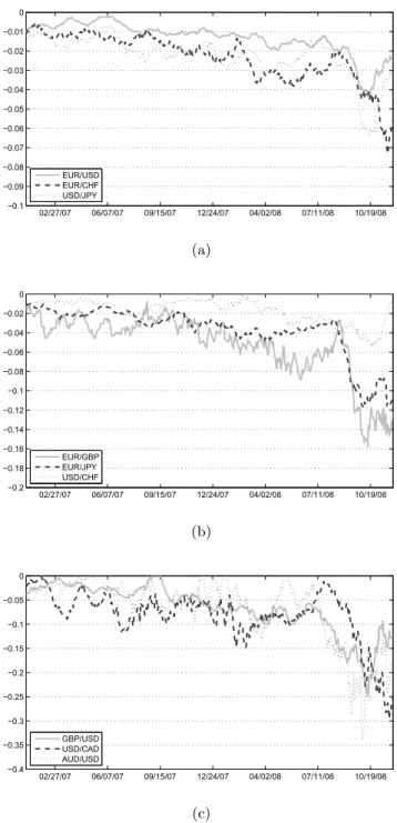
All daily liquidity measures of individual exchange rates fluctuate significantly over time. For the return reversal this observation is shared by P´astor and Stambaugh (2003) who conclude that their reversal measure is a rather noisy proxy for liquidity at the individual asset level. To alleviate this problem, overlapping weekly and monthly liquidity series are constructed by computing time-series averages of the daily estimates. This “within exchange rate” averaging has similar effects as P´astor and Stambough’s (2003) approach of computing the cross-sectional mean across stocks. From Figures 1 and 2, which depict weekly and monthly liquidity, respectively, this smoothing effect becomes apparent.

[Figure 1 about here.]

[Figure 2 about here.]

While the weekly estimates are still rather noisy, the overlapping monthly estimates exhibit less variation. Most currencies are relatively stable and liquid at the beginning of the sample. However, after the subprime crisis started to significantly effect financial markets in the course of 2007, a downward trend in liquidity becomes visible for all exchange rates. In line with Melvin and Taylor

(2009), who identify August 16, 2007 to be the start of the crisis in FX markets, liquidity decreased during the major unwinding of carry trades in August 2007. In the following months liquidity tended to rebound for most currency pairs before starting a downward trend in the end of 2007. This decline was mainly due to changes in risk appetite and commodity related selling of investment currencies which led investors to deleverage by unwinding carry trades. The decrease in liquidity continued after the collapse of Bear Stearns in March 2008. In the second quarter of 2008 investors started to believe that the crisis might be over soon, thus, liquidity increased as investors began to invest again in FX markets. However, in September 2008, liquidity dramatically dropped following the default of Lehman Brothers. This decline reflects the unprecedented turmoil in financial markets caused by the bankruptcy.

Figure 1 and especially Figure 2 suggest that liquidity co-moves across currencies. Consequently, commonality in FX liquidity will be investigated in the next section.

4.

Commonality in foreign exchange liquidity

Testing for commonality in FX liquidity is crucial as the presence of shocks to market-wide liquidity has important implications for investors as well as regulators. Therefore, a time-series of systematic FX liquidity is constructed representing the common component in liquidity across different exchange rates.

4.1. Averaging liquidity across currencies

In the first approach, an estimate for market-wide FX liquidity is computed simply as the cross-sectional average of liquidity at individual exchange rate level. This method of determining aggregate liquidity has been applied to equity markets by Chordia, Roll, and Subrahmanyam (2000) as well as P´astor and Stambaugh (2003). Formally, systematic liquidity based on liquidity measure L is

estimated as follows: LM t = 1 N N j=1 Lj,t, (10)

where N is the number of exchange rates. In order for common liquidity to be less influenced by extreme currency pairs, it is estimated by relying on a trimmed mean. More precisely, the currency pairs with the highest and lowest value forL_j,t are excluded in the computation of LM_t . Systematic FX liquidity based on different measures is depicted in Figure 3. The sign of each measure is adjusted such that the measure represents liquidity rather than illiquidity. Consequently, an increase in the measure is associated with higher liquidity.

[Figure 3 about here.]

Bid-ask spreads, volatility and the trade impact coefficient increase towards the end of the sample, which is in line with the decrease in the reversal measure. All measures uniformly indicate a steep decline in liquidity after September 2008 when the default of Lehman Brothers as well as the rescue of American International Group (AIG) took place. The stabilization of liquidity at the very end of the sample might be related to governments’ efforts to support the financial sector, for instance by initiating the Troubled Asset Relief Program (TARP) in the United States.

Compared to P´astor and Stambough’s (2003) reversal measure for equity markets, aggregate FX return reversal for monthly data is negative over the whole sample. This desirable result might be caused by the fact that the EBS data set includes more accurate order flow data and that Model (1) is estimated robustly at a higher frequency.

Given the estimate of market-wide FX liquidity, basic empirical evidence for commonality in FX liquidity can be obtained by regressing percentage changes in liquidity of individual exchange rates on changes in systematic liquidity:

whereDL_j,t ≡(L_j,t−L_j,t−1)/L_j,t−1 is the relative change of liquidity measureLfor exchange ratej. Analogously,DLM_t is defined for relative changes in market liquidity, which are computed excluding currency pair j. Similar to Chordia, Roll, and Subrahmanyam (2000), relative changes in liquidity, rather than levels, are investigated as the objective is to highlight co-movement in liquidity. Table 3 shows the regression results.

[Table 3 about here.]

The cross-sectional average of the slope coefficientsβ_j is positive and significant for all measures. Of the individual β_j’s approximately 89% are positive and 78% are positive as well as significant based on the reversal measure while all slopes are positive and significant for the alternative mea-sures. Average adjusted-R2s are higher than those for daily equity liquidity of Chordia, Roll, and Subrahmanyam (2000). This finding might be explained by the fact that daily noise is averaged out at the monthly horizon. Moreover, the nature of the FX market including triangular connections between exchange rates might partially induce some commonality in liquidity. These results are indicative of strong commonality in FX liquidity. The next section investigates commonality more rigorously by relying on principle component analysis.

4.2. Latent liquidity

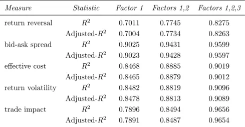
Instead of averaging, Hasbrouck and Seppi (2001) as well as Korajczyk and Sadka (2008) rely on principle component analysis (PCA) to document commonality. To that end, liquidity measure L for each exchange rate is standardized by the time-series mean and standard deviation of the average of measure L obtained from the cross-section of exchange rates. Then, the first three principle components across exchange rates are extracted for each liquidity measure. Finally, for each currency pair, the time-series of liquidity measure L is regressed on the principle components. To assess the level of commonality, the cross-sectional average of the coefficient of determination as well as the

adjusted-R2 are shown in Table 4.

[Table 4 about here.]

Similar to the regressions in the previous section, Table 4 reveals ample evidence of strong com-monality. The first principle component explains between 70% and 90% of the variation in monthly FX liquidity depending on which measure is used. As additional support, the (adjusted-) R2 in-creases further when two or three principle components are included as explanetory variables. As in the previous section, the reversal measure exhibits the lowest level of commonality. Moreover, the R2 statistics are again significantly larger than those for equity data computed by Korajczyk and Sadka (2008). To summarize, all empirical results suggest a high level of commonality in FX liquidity. This commonality is stronger than in equity markets when comparing the results of this paper to the studies by Chordia, Roll, and Subrahmanyam (2000), Hasbrouck and Seppi (2001) as well as Korajczyk and Sadka (2008).

Korajczyk and Sadka (2008) take the idea of using PCA to extract common liquidity one step further by combining the information contained in various liquidity measures. Empirical evidence on commonality and visual inspection of Figure 3 show that alternative liquidity measures yield qualitatively similar results. Indeed, the correlation between different aggregate liquidity measures is around 0.8 for weekly and 0.9 for monthly data. This high correlation indicates that all measures proxy for the same underlying latent liquidity factor. Unobserved systematic liquidity can be ex-tracted by assuming a latent factor model for the vector of standardized liquidity measures, which can again be estimated using PCA. Given that the first principle component explains the majority of variation in liquidity of individual exchange rates, the first latent factor is used as measure for systematic liquidity. Similar to the simple measures, the sign of the factor is chosen such that it represents liquidity. Figure 4 illustrates latent market-wide FX liquidity over time together with the Chicago Board Options Exchange Volatility Index (VIX) as well as the TED-spread.

[Figure 4 about here.]

The graph of systematic FX liquidity estimated by PCA resembles the one obtained by averaging liquidity of individual exchange rates. Again market-wide FX liquidity decreases after the beginning of the subprime crisis and there is a steep decline in the aftermath of the collapse of Lehman Brothers. This similarity in estimated common liquidity is confirmed by correlations between 0.8 and 0.9 depending on which measure is used when averaging. More remarkable is the relation to the VIX and the TED-spread. Primarily an index for the implied volatility of S&P 500 options, the VIX is frequently used as a proxy for investors’ fear inherent in financial markets, whereas the TED-spread proxies the level of credit risk and funding liquidity in the interbank market. During most of 2007 and 2008, the severe financial crisis is reflected in a TED-spread which is significantly larger than its long-run average of 30–50 basis points.

Interestingly, the VIX as well as the TED-spread are strongly negatively correlated with FX liquidity (approximately −0.8 and−0.7 for latent liquidity) indicating that investors’ fear measured by implied volatility of equity options and credit risk has spillover effects to other financial markets as well. The increasing integration of international financial markets might be a reason for this linkage as, for instance, the default of Lehman Brothers led to severe repercussions in all financial markets. To investigate this issue further, the relation between systematic FX liquidity and liquidity of equity markets is investigated in the next section.

4.3. Relation to liquidity of the US equity market

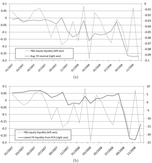
Given the high correlation to the VIX, it is promising to investigate commonality in liquidity across different financial markets. To that end, the measures of market-wide FX liquidity presented in the previous subsections are compared to systematic liquidity of the US equity market. The latter is estimated based on return reversal (P´astor and Stambaugh, 2003) utilizing return and volume data of all stocks listed at the New York Stock Exchange (NYSE) and the American Stock Exchange

(AMEX)8. Figure 5 shows a comparison of liquidity in FX and equity markets based on a sample of 24 non-overlapping observations.

[Figure 5 about here.]

The results support the notion that liquidity shocks are systematic across markets. Moreover, the correlation between equity and FX liquidity is 0.46 and 0.34 depending on whether the latter is obtained from averaging return reversal or from principle component analysis across different liquidity measures. Similarly, a Spearman’s rho of 0.40 and 0.41 indicates co-movement, further substantiating the finding of integrated financial markets.

Having analyzed liquidity of individual exchange rates and illustrated the strong degree of com-monality across exchange rates as well as with equity liquidity, the question arises whether systematic liquidity risk is priced in the cross-section. The presence of such a liquidity risk premium in FX mar-kets would further underline the importance of the previous analysis.

5.

Liquidity risk premiums

5.1. Monthly data

To investigate the role of liquidity in cross-sectional asset pricing, monthly dollar log-returns are constructed from daily spot rates in units of foreign currency per USD. Hence, in contrast to the pre-vious analysis, all returns are based on USD as base currency, which allows for better interpretation of the factors. Additional to FX data, interest rates are necessary to construct risk factors and to analyze liquidity risk premiums as well as excess returns over UIP. Thus, similar to Liu and Maynard (2005) the interest rate differential for the various currencies is computed from LIBOR interest rates, which are obtained from Datastream. LIBOR rates are converted to continuously compounded rates

8_{Current estimates for the equity liquidity factor are obtained from ˇLuboˇs P´astor’s website: http://faculty.}

to allow for comparison with monthly FX log-returns, which are computed at the same point in time. Combining these data sets, the variable of interest is the excess return over UIP:

re

j,t+1=ift −idt −Δpj,t+1, (12)

whereif_t andid_t represent the one-month foreign and domestic LIBOR interest rates at dayt, respec-tively. r_j,te ₊₁ denotes the one month excess return of currency pair j at day t from the perspective of US investors. Alternatively, it can be interpreted as the return from a carry trade in which a US investor who borrows at the domestic and invests in the foreign interest rate is exposed to exchange rate risk. For the purpose of the asset pricing study, gross excess returns are used, because excess returns net of bid-ask spreads overestimate the true cost of trading. In practice, foreign exchange swaps are often preferred over spot trading to maintain currency portfolio positions due to their minimal trading cost (Gilmore and Hayashi, 2008). Descriptive statistics for exchange rate returns, interest rate differentials as well as excess returns are depicted in Table 5.

[Table 5 about here.]

Panel I shows that the annualized returns of individual exchange rates between January 2007 and December 2008 are very large in absolute value compared to the longer sample of Lustig, Roussanov, and Verdelhan (2009). While prior to the default of Lehman Brothers (Panel II) the difference in magnitude is rather small, extreme average returns of up to 85% per annum occur after the collapse (Panel III). In general, the interest rate differentials are lower in absolute value in the last subsample mirroring the joint efforts of central banks to alleviate the economic downturn by lowering interest rates. Typical carry trade funding currencies of low interest rate countries (JPY and CHF) have a positive excess return while the excess return is negative for investment currencies which are associated with high interest rates (AUD, NZD). This holds true for the whole sample, but the

differences are more substaintial after September 2008. These negative excess returns indicate an increased risk and deteriorated profitability of carry trades.

These significant excess returns over UIP in combination with the large literature on risk-based explanations of this failure warrants further analysis. Therefore, a factor model for excess FX returns including liquidity risk is presented next.

5.2. Risk factors for foreign exchange returns

Following the arbitrage pricing theory of Ross (1976), variation in the cross-section of returns is assumed to be caused by different exposure to a small number of risk factors. To estimate a factor model and to quantify the market prices of risk, potential factors to explain excess exchange rate returns are introduced in this section.

The first two risk factors are similar to the ones introduced by Lustig, Roussanov, and Verdelhan (2009). The “market risk factor”AER_t is constructed as

AERt= 1 N N j=1 re j,t, (13)

and describes the average excess return, i.e. the return for a US investor who goes long in all N exchange rates available in the sample. The second risk factor, HML_t, is the excess return of a portfolio which is long the two exchange rates with the largest interest rate differential and short the two exchange rates with the smallest interest rate differential. Therefore, it can be interpreted as a “slope” or “carry trade risk factor”; see Lustig, Roussanov, and Verdelhan (2009) for further details on the interpretation and construction of these two factors.

Investors might require only a small premium for the absolute level of liquidity of individual exchange rates as cross-sectional differences can be accounted for in portfolio strategies. In contrast, the risk of market-wide shocks to liquidity might command a significant risk premium. Therefore, to

obtain a liquidity risk factor, the estimates for systematic liquidity presented above are decomposed into expected changes and unanticipated shocks. Similar to the approaches of P´astor and Stambaugh (2003) as well as Acharya and Pedersen (2005), a “common liquidity shock risk factor” CLSP CA

t

is defined to be the residuals from an AR(2) model fitted to latent systematic liquidity. CLS_tAV G is analogously defined when using the average liquidity of individual exchange rates as proxy for aggregate liquidity. Estimating an AR(2) model for the level of systematic liquidity is equivalent to an AR(1) model for ΔLM_t . Thus, CLS_t captures the unpredicted change of liquidity in month t. Figure 6 depicts the time series of risk factors.

[Figure 6 about here.]

In particular after the collapse of Lehman Brothers, there are negative shocks to aggregate liquid-ity independent of which measure has been used to proxy for aggregate liquidliquid-ity. While the twoCLS measures differ to some extent in the beginning and middle of the sample, they co-move closely after September 2008. Moreover, the average excess return as well asHMLare negative during the latter subperiod. The carry trade risk factor seems to be influenced by liquidity as the two exhibit a rather strong correlation of 0.43 for CLSAV G and 0.51 for CLSP CA. Hence, to separate the influences of general macro risk and liquidity effects, HML is orthogonalized to CLS. To that end, HMLO_t is defined to be the residuals of the following regression:

HMLt=α0+α1CLSt+ut. (14)

In particular after the default of Lehman Brothers, the orthogonalized slope factor, HMLO_{, is not}

as negative asHML, which can be explained by the fact that liquidity plays an important role in the increased risk after the default of Lehman Brothers. Furthermore, the period of large unexpected shocks to aggregate liquidity coincides with a depreciation of USD against the basket of foreign

currencies.

Having described candidate risk factors for explaining excess returns in FX markets, the next section introduces asset pricing models to assess the relative importance of the factors and to compute their associated market prices of risk.

5.3. Cross-sectional asset pricing and market prices of risk

This section investigates whether investors demand a return premium for being exposed to liquidity risk. To that end, asset pricing models based on the previously introduced factors will be estimated. As a first step, the model of Lustig, Roussanov, and Verdelhan (2009) is augmented by a liquidity risk factor. The effect of additionally introducing volatility risk (Menkhoff, Sarno, Schmeling, and Schrimpf, 2009) is investigated in the robustness anaylsis in Section 6. Letting δ_AER,t, δ_{HM L,t}, and

δCLS,t denote the market prices of risk, the asset pricing model of interest is:

Ere j

=δ_AERβ_AER,j+δ_{HM L}β_{HM L,j}+δ_CLSβ_CLS,j, (15)

Excess returns of individual exchange rates are used as dependent variables. Compared to the more common approach of using portfolios, relying on individual excess returns increases the dispersion around beta estimates, however, the asymptotic standard errors of factor risk premiums will be lower (Ang, Liu, and Schwarz, 2008). The betas can be obtained from a time-series regression of excess returns on the factors:

re

For estmation purposes, it is more convenient to express this expected return-beta factor model in an equivalent stochastic discount factor (SDF) representation (Cochrane, 2005):

mt= 1−bAERAERt−bHMLHMLt−bCLSCLSt. (17)

The factor loadings in the SDF, b = [b_AER b_HML b_CLS], and the market prices of risk, δ = [δ_AER δ_{HM L} δ_CLS], are related by

δ=E[ff]b,

where E[ff] denotes the variance-covariance matrix of the factors. While b_k can be used to test whether factor k helps to price assets given the other factors, a significant δ_k indicates whether factor k is priced in the cross-section.

Without arbitrage opportunities, the excess return of currency j satisfies the following pricing equation: Et mt+1rj,te +1 = 0. (18)

Consequently, the Generalized Method of Moments (GMM) of Hansen (1982) naturally lends itself as an ideal estimation technique for the parameters in the SDF framework. Relying on Equation (18) as moment conditions, GMM estimates are found by minimizing the weighted sum of squared pricing errors. Usually, the solution is found in a two-step procedure. In the first step, the weighting matrix, W, is chosen to be the identity matrix, yielding consistent and asymptotically normal first-step GMM estimates as solution to the minimization problem. Asymptotic efficiency with regard to the specified set of moment conditions can be achieved by using the inverse of the long-run variance-covariance matrix of the excess returns in the moment conditions as weighting matrix. Given the estimated parameters from step one, this long-run variance-covarinace matrix is estimated using the Newey–West estimator together with the Bartlett kernel (Newey and West, 1987). To increase the

sample size, overlapping monthly returns are computed for every trading day t. Moving average effects are accounted for by reporting Newey and West (1987) standard errors with 21 lags.

Recalling the differences in descriptive statistics and due to the severe implications of the Lehman Brothers collapse for every financial market, a structural break in September 2008 is expected. Contrary to Bear Stearns, the Federal Reserve and US Treasury did not treat Lehman Brothers as “too big to fail” creating turmoil in financial markets that was unlike anything witnessed before (Melvin and Taylor, 2009). Unfortunately, it is not possible to formally test for such a breakpoint as there are not enough observations to reliably estimate the model for the subsample after the default of Lehman Brothers for comparison. Nevertheless, the focus of the interpretation lies on the estimation results for the subsample prior to September 13, 2008. Table 6 shows two-stage GMM regression results for alternative specifications of the asset pricing model for this subsample. First-stage GMM results are similar and are therefore omitted for brevity, but are available from the authors upon request.

[Table 6 about here.]

The first column of Table 6 reports estimation results for the benchmark model of Lustig, Rous-sanov, and Verdelhan (2009). In line with their results, the carry trade risk factor receives a positive premium of 18% per year. However, similar to the market risk factor, the market price of carry trade risk is not significantly different from zero. On the contrary, the positive estimate for the market price is significant for the models including liquidity risk only, which are shown in columns two and three. Both using latent liquidity risk as well as aggregate liquidity risk obtained by averaging lead to significant market prices of liquidity risk. A currency pair with aβ_CLS of one earns a risk premium of 7% and 13% per year, depending on whether latent or average liquidity is used for constructing common liquidity shocks. Furthermore, the factor loadings in the SDF are positive and significant. These results suggest an important role of liquidity risk while the general slope factor representing

macro risk has difficulties in explaining the variation in excess returns of individual exchange rates. To support the previous results, columns four to seven of Table 6 show estimation results for asset pricing models including a combination of three factors. The models in columns four and six augment the asset pricing model of Lustig, Roussanov, and Verdelhan (2009) by a liquidity risk factor. Now, the market prices of slope and market risk are of the same magnitude as the ones found by Lustig, Roussanov, and Verdelhan (2009), however, both are not significant. On the other hand, CLSAV G

and CLSP CA receive a significant premium of 10% and 27% in models four and six, respectively. Moreover, the SDF factor loadings for liquidity risk are positive and significant as well, whereas they are negative and/or not significant for HML. Furthermore, the fourth model including unexpected shocks to average liquidity yields the smallest pricing errors of all models. Lastly, models five and seven include the orthogonalized versions of the carry trade factor. AsHMLO

t is not an excess return,

one moment condition is lost for the GMM estimation. Again liquidity risk is priced while the results for HMLO_t contradict each other. Overall, the estimation results are clearly indicative of liquidity risk receiving a significant risk premium of as high as 20% per year. This premium is large compared to equity liquidity risk premiums (see for instance P´astor and Stambaugh (2003) and Acharya and Pedersen (2005)), which might be explained by the particular sample period investigated in this paper. Additionally, liquidity risk helps to price assets in the cross-section of excess exchange rate returns.

The presence of strong liquidity risk effects is even more remarkable, because every measure of liquidity will always be an approximation. Thus, the effect of liquidity is in general hard to detect, since errors in variables typically lead to a downward bias in the estimated regression coefficients (Amihud, Mendelson, and Pedersen, 2005). Consequently, finding significant liquidity risk premiums in a crisis period, which is a challenge for every model, underlines the quality of the liquidity measure based on return reversal introduced above. Moreover, given that continuously compounded returns and mid-quotes are used in the asset pricing study, the liquidity risk premia are not subject to the

potential upward bias described by Asparouhova, Bessembinder, and Kalcheva (2009).

Compared to the results of using latent systematic liquidity extracted from various different measures, the results of utilizing unexpected shocks to average return reversal are qualitatively similar and even lead to smaller pricing errors. Therefore, for the sample at hand it is not necessary to compute various liquidity measures and conduct a PCA, as very similar results are obtained when using solely the reversal measure. Moreover, the latter has the advantage of a clearer interpretation compared to latent liquidity.

Given the extreme nature of excess returns after the default of Lehman Brothers, none of the models provides a good fit for the whole sample, supporting the hypothesis of a structural break. J -statistics reject the null hypothesis of zero pricing errors for all models. GMM estimates are available form the authors upon request. These results are not surprising as risk aversion and volatility rose to incredible levels in the aftermath of the default of Lehman Brothers. Dramatic fear in the market lead to extreme market conditions and an unprecedented deleveraging imposing large losses on firms across the industry.

The next section presents evidence regarding the robustness of the results.

6.

Robustness analysis

6.1. Robustness of the return reversal liquidity measure

To analyze the robustness of the liquidity estimates obtained from the return reversal measure, Model (1) is estimated only using the ten most busy trading hours of the day. Table 7 shows that the return reversal measure as well as the alternative measures indicate marginally higher liquidity, but the differences are of small magnitude.

Moreover, the liquidity estimates obtained from the return reversal measure are robust to the choice of sampling frequency. Specifically, Panel I of Table 8 shows that the results are qualitatively similar and all conclusions remain valid when estimating Model (1) based on five-minute return and order flow data. For most currencies the return reversal is even more pronounced compared to one-minute data.

[Table 8 about here.]

Lastly, Model (1) is estimated using OLS regression. As anticipated, the estimates for return reversal and trading impact are more volatile over time compared to the robust estimates. Panels II and III of Table 8 show that the standard deviations of return reversals obtained using OLS are significantly larger, highlighting the fact that robust estimation leads to fewer extreme values as robust regression is less affected by extreme observations. Consequently, relying on robust regression techniques is preferable.

Having established the robustness of the return reversal liquidity measure, the next section in-vestigates the robustness of commonality in FX liquidity.

6.2. Robustness of commonality in FX liquidity

Being derived from liquidity of individual exchange rates, the proxies for market-wide liquidity are robust to the estimation technique and sampling frequency of the individual liquidity measures as well. Figure 7 contrasts the evolution of estimates for systematic liquidity based on different sampling frequencies and estimation techniques.

[Figure 7 about here.]

When using five-minute data or OLS estimation, the characteristics of the common liquidity series do not change significantly, thus, estimated market-wide FX liquidity continues to mirror important crisis events. Next, the stability of liquidity risk premiums will be investigated.

6.3. Robustness of liquidity risk premiums

To test the robustness of liquidity risk premiums, the factor models for FX excess returns are re-estimated using different base currencies. As before, Tables 9 and 10 indicate the presence of liquidity risk premiums when using CHF or AUD as base currency. These currencies are of particular interest as they represent funding and investment currencies of carry trades. Thus, the conclusion that liquidity risk receives a significant risk premium is robust to the choice of base currency.

[Table 9 about here.]

[Table 10 about here.]

In a recent study, Menkhoff, Sarno, Schmeling, and Schrimpf (2009) highlight the role of volatility risk premiums in FX returns. Therefore, it is analyzed whether the finding of a significant liquidity risk premium prevails when including FX volatility risk in the asset pricing model. Common volatility shocks (CVS_t) are constructed by fitting an AR(2) model to average option implied volatility from one-month exchange rate options. Table 11 shows two-stage GMM estimation results for a number of FX asset pricing models including volatility risk.

[Table 11 about here.]

In Model (1), only volatility risk is included as risk factor. In line with Menkhoff, Sarno, Schmel-ing, and Schrimpf (2009), the price of volatility risk,δ_CVS, is negative and significantly different from zero. When adding liquidity risk factors to the model, δ_CVS decreases in absolute value and even becomes insignificant in Model (3), which includes latent market-wide liquidity risk. On the other hand, CLS and CLS_latent are significantly priced in Models (2) and (3), respectively. The market price of liquidity risk is also positive in the full models (4) and (5), which additionally include the market and carry trade risk factors proposed by Lustig, Roussanov, and Verdelhan (2009). In Model (4), volatility risk is insignificant, whereas there is some evidence for volatility risk being a priced

risk factor in Model (5). All in all, including volatility risk corroborate the finding that shocks to market-wide liquidity are an important risk factor. Similar results are obtained when including un-expected changes of theV IX as a risk factor in the asset pricing models. Estimation results are not shown, but can be obtained from the authors upon request.

As alternative to using overlapping monthly data, the asset pricing analysis is repeated with non-overlapping weekly data. GMM estimation results are shown in Table 12. Due to the fact that there are only 83 observations, first-stage GMM is preferable over two-stage GMM for robustness considerations (Cochrane, 2005). Again, the estimation results are indicative of large FX liquidity risk premiums. However, as had to be expected, the standard errors are large due to the short sample and the noise inherent in weekly return data.

[Table 12 about here.]

As further robustness check secured overnight index swaps (OIS) could be used instead of LIBOR rates for the computation of excess exchange rate returns. During the financial crisis, LIBOR rates tended to be larger than OIS rates due to embedded risk premiums. However, the magnitude of interest rates compared to FX returns is very small, in particular after the default of Lehman Brothers where differences between OIS and LIBOR are most pronounced. Consequently, the choice of interest rate does not qualitatively affect the finding of a significant liquidity risk premium.

7.

Conclusion

The recent financial crisis confirms that illiquidity is ubiquitous in all financial markets during dis-tressed market conditions. Contrary to the common perception of the FX market being extremely liquid at all times, this paper shows that liquidity is an important issue in the FX market. To that end, a liquidity measure particularly tailored to the foreign exchange market is developed, the amount of commonality in liquidity across different exchange rates is quantified, and the extent of

liquidity risk premiums inherent in FX returns is determined. The new liquidity measure is based on intra-day return reversal and captures cross-sectional and temporal variation in FX liquidity. Utiliz-ing an ultra high frequency dataset, the importance of liquidity in the FX market is highlighted by the fact that FX liquidity declined severely during the financial crisis of 2007–2008. This finding is not only true for individual exchange rates, but also for market-wide liquidity. Indeed, liquidity in exchange rates can be decomposed into an idiosyncratic and a common component. This high degree of commonality also has important implications for asset pricing as investors are averse to shocks to market-wide liquidity. To investigate whether investors require a return premium for bearing liquid-ity risk, a factor model for FX returns is extended by a novel liquidliquid-ity risk factor constructed from shocks to market-wide liquidity. Estimation results suggest that liquidity risk is a heavily priced state variable, stressing the importance of liquidity risk in the determination of FX returns. Furthermore, this finding supports risk-based explanations for deviations from Uncovered Interest Rate Parity.

These results have several important implications. First, the new liquidity measure allows central banks and regulatory authorities to assess the effectiveness of their policy by enabling them to monitor liquidity on a daily basis. Second, stressing the important role of liquidity helps liquidity providers and speculators such as carry traders to more adequately understand the risk of their trading, which is crucial in light of the potential losses from currency crashes coinciding with liquidity spirals.

References

Acharya, V. V., and L. H. Pedersen, 2005, “Asset Pricing with Liquidity Risk,”Journal of Financial

Economics, 77(2), 375–410.

A¨ıt-Sahalia, Y., P. A. Mykland, and L. Zhang, 2005, “How Often to Sample a Continuous-Time Process in the Presence of Market Microstructure Noise,”The Review of Financial Studies, 18(2), 351–416.

Amihud, Y., 2002, “Illiquidity and Stock Returns: Cross-Section and Time-Series Effects,” Journal

of Financial Markets, 5(1), 31�