Wind Levelized Cost of Energy: A Comparison of Technical and Financing Input Variables

(1)

Technical Report

NREL/TP-6A2-46671 October 2009

Wind Levelized Cost of Energy:

A Comparison of Technical and

Financing Input Variables

(2)

National Renewable Energy Laboratory

1617 Cole Boulevard, Golden, Colorado 80401-3393 303-275-3000 • www.nrel.gov

NREL is a national laboratory of the U.S. Department of Energy Office of Energy Efficiency and Renewable Energy

Operated by the Alliance for Sustainable Energy, LLC Contract No. DE-AC36-08-GO28308

Technical Report

NREL/TP-6A2-46671 October 2009

Wind Levelized Cost of Energy:

A Comparison of Technical and

Financing Input Variables

Karlynn Cory and Paul Schwabe

(3)

NOTICE

This report was prepared as an account of work sponsored by an agency of the United States government. Neither the United States government nor any agency thereof, nor any of their employees, makes any warranty, express or implied, or assumes any legal liability or responsibility for the accuracy, completeness, or usefulness of any information, apparatus, product, or process disclosed, or represents that its use would not infringe privately owned rights. Reference herein to any specific commercial product, process, or service by trade name, trademark, manufacturer, or otherwise does not necessarily constitute or imply its endorsement, recommendation, or favoring by the United States government or any agency thereof. The views and opinions of authors expressed herein do not necessarily state or reflect those of the United States government or any agency thereof.

Available electronically at

Available for a processing fee to U.S. Department of Energy and its contractors, in paper, from:

U.S. Department of Energy

Office of Scientific and Technical Information P.O. Box 62

Oak Ridge, TN 37831-0062 phone: 865.576.8401 fax: 865.576.5728

email:

Available for sale to the public, in paper, from: U.S. Department of Commerce

National Technical Information Service 5285 Port Royal Road

Springfield, VA 22161 phone: 800.553.6847 fax: 703.605.6900

email:

online ordering:

(4)

iii

Acknowledgments

This work was funded by the U.S. Department of Energy’s (DOE’s) Wind and Hydropower Technologies Program. The authors thank Maureen Hand, of the National Renewable Energy Laboratory (NREL), for her guidance and overall direction provided to this project. The authors also thank Walter Short of NREL for providing useful insights and helpful input on wind project financing. In addition, the authors thank Matthew Karcher of Deacon Harbor Financial for his continued support and guidance in using his wind project finance model. Finally, the authors thank the individuals who reviewed various drafts of this report including Douglas Arent, Maureen Hand, David Kline, Margaret Mann, Michael Mendelsohn, and James Newcomb of NREL; Matthew Karcher of Deacon Harbor Financial; and Mark Bolinger and Ryan Wiser of Lawrence Berkeley National Laboratory.

The authors also thank Michelle Kubik of NREL for her editorial support and Jim Leyshon of NREL for his graphics support.

(5)

iv

List of Acronyms and Abbreviations

BL back leveraged

Cash Lev cash leveraged

Corp corporate

DOE Department of Energy IEA International Energy Agency IIF institutional investor flip IOU investor-owned utility IRR internal rate of return IRS Internal Revenue Service LCOE levelized cost of energy

NREL National Renewable Energy Laboratory O&M operations and maintenance

PTC Lev production tax credit leveraged PTC production tax credit

REC renewable energy certificate SIF strategic investor flip

(6)

v

List of Figures

Figure ES-1. LCOE Sensitivities for capacity factor, installed cost, O&M, and target IRR by financing structure ... vi

Figure ES-2. Technical- vs. financial-variables scenario analysis ... vii

Figure 1. LCOE ranges by individual variable sensitivities, showing all financing structures ...8

Figure 2. Institutional Investor Flip LCOE sensitivities by input variable ...9

Figure 3. Cash Leveraged structure LCOE sensitivities by input variable ...10

Figure 4. LCOE sensitivities for capacity factor, installed cost, O&M, and target IRR by financing structure ...11

Figure 5. Multivariable scenarios LCOE ranges ...12

Figure 6. Technical- vs. financial-variables scenario analysis ...14

Figure C1. Corporate structure LCOE sensitivities by input variable ...23

Figure C2. Strategic Investor Flip structure LCOE sensitivities by input variable ...24

Figure C3. Cash and PTC Leveraged structure LCOE sensitivities by input variable ...25

List of Tables

Table 1. Technical Variables: Individual Variable Sensitivities ...5

Table 2. Financial Variables: Individual Variable Sensitivities ...5

Table 3. Technical Variables: Multivariable Scenarios ...6

Table 4. Financial Variables: Multivariable Scenarios ...6

Table 5. Base-Case LCOE Estimates ...7

Table A1. Input Assumptions Common to All Structures ...18

Table A2. Structure-Specific Equity-Financing Assumptions ...19

Table A3. Structure-Specific Debt-Financing Assumptions ...20

Table B1. Technical Variables: Individual Variable Sensitivities ...21

Table B2. Financial Variables: Individual Variable Sensitivities ...21

(7)

vi

Executive Summary

As part of a multinational collaborative study, the National Renewable Energy Laboratory (NREL) conducted a comparison of the relative impacts of various financial, technological, and wind resource variables on the levelized cost of energy (LCOE) 1_{from a typical wind project.} The parametric analysis identified and compared key factors in the cost of wind energy in the United States. Analysts used a LCOE pro forma cash flow model to reflect recent U.S. wind project financing structures and wind energy market trends. However, the financial crisis of 2008-2009 and subsequent U.S. federal legislation is not considered in detail because it is still early to discern and model the exact impacts.

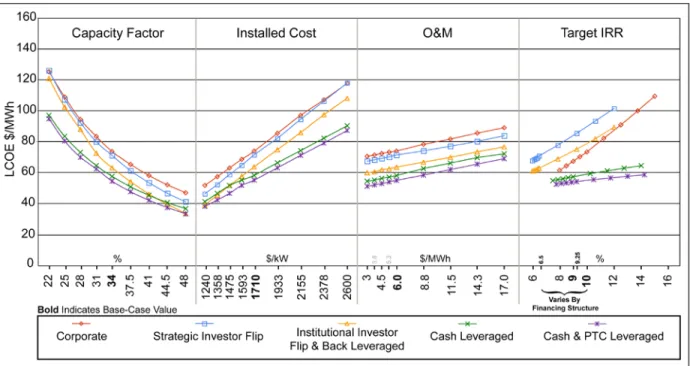
Analysts first examined the impacts of wind resource, financial, and technical variables on the LCOE independently. Each variable’s impact was tested across a range of high- and low-cost values for six wind project financing structures, which are described in the report. As expected, the wind resource variable and all-in installation costs have the largest incremental effect on LCOE. These technical variables reveal that incremental improvements through improved R&D or manufacturing practices can yield sizeable cost savings, especially for those projects with below-average wind resource characteristics. A less obvious, yet moderate LCOE impact resulted from variations in the target equity internal rate of return (IRR), the operations and maintenance costs (O&M), as well as the return on debt and loan duration (debt-financed structures only). The smallest impact resulted from the cost of replacing a specific wind turbine component. Figure ES-1 plots the input variables with the largest impact on the estimated LCOE.

Figure ES-1.LCOE Sensitivities for capacity factor, installed cost, O&M, and target IRR by financing structure

1_{As described in the report, LCOE is calculated as the project’s contracted price of energy that yields the required} internal rate of return for the project’s developer or tax equity investor.

(8)

vii

In addition to individual variable sensitivities, a multivariable scenario analysis estimated the combined effect of varying an entire set of inputs simultaneously on the projected LCOE. For the multivariable scenario analysis, the input parameters’ respective highest and lowest cost values were modified to be closer to a base-case estimate; this helped model realistic and potentially achievable project characteristics, when tested simultaneously. Analysts modeled three cost scenarios, which represent the optimal (e.g., high performance, low installed cost, and low finance costs), average, and inferior wind projects – each returned markedly different LCOEs. The estimated LCOEs from the three cost scenarios ranged from cost-competitive with 2008 U.S. wholesale power prices to more than twice as high as wholesale prices. Therefore, it is difficult to make generalizations about wind LCOE because the cost of a wind project is very site-specific.

Lastly, analysts evaluated two subgroupings of the multivariable scenarios (shown in Figure ES-2): technical variables (wind resource, installation and equipment replacement costs, O&M) and financial variables (IRR, debt terms). The analysis examined which subset of variables had a larger impact on the estimated LCOE. For each financing structure tested, the impact of the set of technical variables was several times larger than the set of financial variables on the estimated LCOE. The relative impacts of the financing variables were maximized under the two structures that incorporate debt financing; however, to date, wind projects have not commonly used debt at the project level.

0 20 40 60 80 100 120 140 160 180 Corporate Strategic Investor Flip

Institutional Investor Flip & Back Leveraged

Cash Leveraged Cash & PTC Leveraged

LC

O

E $

/M

Wh

Technical Variables LCOE Range Financial Variables LCOE Range Base-Case LCOE

(9)

1

1 Introduction

The expansion of wind power capacity in the United States has increased the demand for project development capital. In response, innovative approaches to financing wind projects have

emerged and are proliferating in the U.S. renewable energy marketplace (Cory et al. 2008). Wind power developers and financiers have become more efficient and creative in structuring their financial relationships, and often tailor them to different investor types and objectives (Harper et al. 2007). As a result, two similar projects may use very different cash flows and financing arrangements, which can significantly vary the economic competitiveness of wind projects. This report assesses the relative impact of numerous financing, technical, and operating variables on the levelized cost of energy (LCOE) associated with a wind project under various financing structures in the U.S. marketplace. Under this analysis, the impacts of several financial and technical variables on the cost of wind energy are first examined individually to better

understand the relative importance of each. Then, analysts examine a low-cost and a high-cost financing scenario, where multiple variables are modified simultaneously. Lastly, the analysis also considers the impact of a suite of financial variables versus a suite of technical variables. The analysis was performed as part of multiyear, multinational International Energy Agency (IEA) task to develop a better understanding of the costs of wind energy. The parametric analysis identified key factors in the cost of wind energy. Future analysis will compare the

country-specific results in an effort to develop a transparent and accepted methodology for estimating wind energy costs and to help project future cost-performance trends.

While this report updates a selected number of assumptions stemming from changes in the financial and wind energy markets since 2007, it does not consider the 2008-2009 financial crisis in-depth. Wind project development has been impacted by the rapid post-September 2008 credit tightening, the simultaneous Wall Street financial turmoil, and subsequent actions by the federal government in 2008 and 2009 to bolster the economy. At the time of this writing, it is still early to discern and model these exact impacts, which will be the subject of many future studies. However, it is apparent that since the financial crisis, the wind industry has seen a dramatic “flight to quality” for new project development (e.g., highly experienced developers, thoroughly tested technology, creditworthy off-takers, etc.) (Schwabe et al. 2009). The combination of these factors impacts the cost of both debt and equity financing; and, thus, the overall LCOE of a wind project.

2 Six Wind Financing Structures Under Study

This analysis incorporates the use of a wind levelized cost of energy model developed in “Wind Project Financing Structures: A Review and Comparative Analysis” (Harper et al. 2007) as well as “A Review of Wind Project Financing Structures in the USA,” (Bolinger et al. 2008). These reports described seven financing structures used in pre-financial crisis wind project

(10)

2

assesses only six financing structures,2_{which are briefly addressed below. For more detailed} descriptions and schematic representations of each structure, see Harper et al. 2007.

All equity-financing structures:

1) Corporate (Corp). A single developer who is able to use all of the project’s tax benefits, and acts as both developer and investor. The corporate developer internally funds 100% of the project’s costs and receives 100% of the project’s associated cash flows and tax benefits.

2) Strategic Investor Flip (SIF). In addition to the project developer, a separate tax equity investor partnered with to fully use a wind project’s tax benefits. The developer and tax equity investor negotiate their respective equity contribution ratios, an initial or “pre-flip” distribution of the project’s cash revenues and tax benefits, and a future or “post-flip” distribution. The “flip-point” occurs once the tax equity investor achieves an agreed upon internal rate of return based on his/her equity contribution.

3a) Institutional Investor Flip (IIF). Also uses a third-party tax equity investor with distinct pre- and post-flip cash and tax benefits allocations. Distinct from the Strategic Investor Flip, the developer in this scenario invests a larger up-front equity investment and tends to attract passive tax equity investors.

3b) Back Leveraged (BL).Identical to the Institutional Investor Flip, but uses corporate-level debt to fund the developer’s equity contribution investment. The loan made to the developer is entirely outside of the project, and is not captured within the model; therefore, these financial structures (3a, 3b) were combined in this analysis.3

Structures with project-level debt:

4) Cash Leveraged (Cash Lev). Similar to the Strategic Investor Flip (partners, cash flows, and tax benefits), except incorporates project-level debt, which is repaid from the wind project’s future cash flows and is collateralized by the project’s assets. This structure boosts equity returns through leveraging of lower-cost capital, and reduces required up-front equity contribution by the developer and/or tax equity investor. In exchange, the project’s debt lender receives interest payments on the loan, preferred claims on cash flows and the project’s assets, and certain project-approval rights.

5) Cash and Production Tax Credit Leveraged (Cash and PTC Lev). Similar to the

Cash Leveraged structure, but additional debt is taken against expected production tax credit (PTC) benefits to fund initial project costs. The goal is to further boost returns and minimize up-front equity contributions. However, developers and tax investors might be

2_{A seventh financing structure, Pay-As-You-Go, has been used primarily as a tool for refinancing wind projects;} therefore, it is excluded in the current evaluation.

3_{Note that for these analyses, the Institutional Investor Flip and Back- Leveraged financing structure are identical at} the project level (the Back-Leveraged structure uses corporate-level debt, which is not captured in the model) and, therefore, return identical results.

(11)

3

required to make future equity contributions if there are any PTC revenue shortfalls (e.g., for project underperformance).

3 Analysis Overview and Assumptions

This analysis examines the impacts of various input parameters as well as the different financing structures on the estimated LCOE. The model used to perform the analysis is an Excel-based pro forma financial cash flow model that uses a representative template for each of the financial structures investigated (Karcher 2008). For each, the model incorporates the assumed rates of return by the developer or tax equity investor, the equity contribution ratios, and the cash and tax benefits allocations, and then solves for the LCOE needed to satisfy those input assumptions (Harper et al. 2007). Each financial analysis uses a combination of shared and structure-specific assumptions to estimate the LCOE. For a detailed description of the model’s input assumptions, see Appendix A.

The model estimates the nominal levelized cost of energy, which includes the all-in cost of the equipment, as well as the cost of financing (both debt interest rate and equity returns), and other ancillary costs (if applicable). Levelized cost of energy also factors in PTC and accelerated depreciation benefits. Because this is a generic analysis without a specific location, several specific elements are excluded, namely state, local, and utility-based incentives; and renewable energy certificate (REC) revenues.

For validation purposes pertaining specifically to this study, renewable energy attorneys from Stoel Rives LLP independently audited the model. Stoel Rives also verified that the assumptions used in the following analyses are representative of the time period under consideration (Stoel Rives 2009).

3.1 Base-Case Assumptions

Analysts used the base-case assumptions as reference points to measure changes in the estimated LCOE from the individual variable sensitivities and the multivariable scenario analyses. In reality, regional or market variations move many projects away from the base case toward more or less cost-competitive wind projects. These variations are captured in the sensitivity and scenario analyses described in Sections 4.1 though 4.3.

The base-case assumptions model a commercial wind project with an in-service date of January 1, 2008. Although more recent year-end 2008 wind data is available, January 1 is used to exclude the effect of the 2008-2009 financial crisis on wind project development (Wiser and Bolinger 2009).

In general, the analysis used assumptions from Harper et al. 2007; however, some of the base-case assumptions were modified to reflect subsequent developments in wind and financing markets. The analysis revised base-case assumptions for the average wind resource, project size, installation costs, equipment replacement costs, and interest and inflation rates. Appendix A includes a detailed listing of the model’s input assumptions.

(12)

4

4 Analysis Methodology, Sensitivity Assumptions, and

Multivariable Scenarios

To estimate the relative impacts of technical and financing variables on the resulting wind power LCOE, analysts modeled both individual variable sensitivities and multivariable scenarios. To model individual variable sensitivities, they developed a range of high-cost, base-case, and low-cost values – based on a variety of industry sources – for each variable studied. They also developed distinct high-cost and low-cost estimates for the multivariable scenarios. The input variables analyzed in the individual and multivariable analyses include:

Technical variables Financial variables

 Capacity factor  Target IRR,4

 Total installed cost  For the two finance structures that use and  Operations & maintenance5_{, and} _{project-level debt:}

 Levelized replacement cost6 _ _{Return on debt (interest rate), and}  Loan duration

The analysts selected these variables for study because they are most likely to impact LCOE, and they must be carefully considered in project development. The Department of Energy (DOE) highlights technical variables of capacity factor, operations and maintenance, and total installed costs as drivers in wind power prices (Wiser and Bolinger 2008, Wiser and Bolinger 2009). Levelized replacement cost, which recovers the expense of technical equipment replacement over the project’s contract life, has also been reported as an increasingly significant component of annual cost of wind energy (Hand 2009).

Because the development of a wind project is capital-intensive, a project’s financing terms are critical to securing investment while developing economically successful projects. For example, debt and equity providers have identified a project’s target IRR as crucial in attracting tax equity that could otherwise flow to separate tax investment opportunities such as affordable housing (Harper et al. 2007); yet high IRRs also increase financing costs. Similarly, the debt terms are key cost factors for developers considering debt financing to fund new project development (Schwabe et al. 2009).

4.1 Individual Variable Sensitivities

For the individual variable sensitivity analysis, the analysis modifies a variable individually to test the stand-alone sensitivity of each input variable on the LCOE (the output). As these variables were individually tested, all other variables were held fixed to the base-case

assumption. These sensitivities were performed to identify which individual variables had the biggest overall impact on LCOE, if modified within a reasonable range.

4_{Target IRR is the negotiated internal rate of return received by the wind project’s investor(s) or developer.} 5_{Operations and maintenance charges are typically distributed between fixed and variable components of the total} O&M cost. For this analysis, variations in O&M expenditures are tested as changes within the variable charges only. 6_{Levelized replacement cost captures expenses associated with technical equipment restitution such as a gear box} replacement or rebuild, but does not account for lost revenue due to equipment downtime.

(13)

5

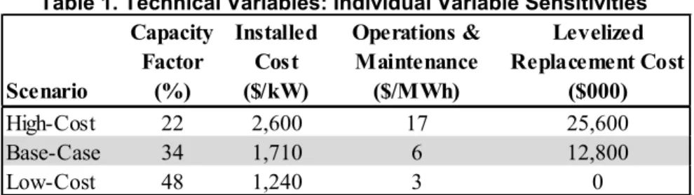
To perform the individual variable sensitivities, analysts developed a range of high-cost, base-case, and low-cost assumptions for each of the input variables. These ranges were based on estimates of realistic wind project characteristics.7_{The financial variable ranges were set wide} enough that it is possible that they encompass the investment conditions that might result from the financial crisis (without attempting to model exactly where the market will finally settle). Table 1 details the high-cost, base-case, and low-cost tested values for the technical input variables.

Table 1. Technical Variables: Individual Variable Sensitivities

Scenario Capacity Factor (%) Installed Cost ($/kW) Operations & Maintenance ($/MWh) Levelized Replacement Cost ($000) High-Cost 22 2,600 17 25,600 Base-Case 34 1,710 6 12,800 Low-Cost 48 1,240 3 0

Table 2 similarly lists the high-cost, base-case, and low-cost tested values for each of the financial variables. Note that the target IRR values are differentiated by financing structure, which is due to each structure’s unique risk and return characteristics among the project investors (Harper et al. 2007). For example, structures with debt carry a greater default risk for the tax equity investor because the project’s debt lenders get priority rights in the case of project default. Therefore, the tax equity investor in the debt-leveraged structures requires a higher target IRR relative to the all-equity financing structure, which compensates for their increased risk exposure. Furthermore, the financing terms (both debt and equity) required by project investors will also vary from project to project within a structure, depending on overall quality of the project, developer reputation, underperformance risk, and other factors.

Table 2. Financial Variables: Individual Variable Sensitivities

Scenario Corp (%) SIF, IIF & BL (%) Cash Lev (%) Cash & PTC Lev (%) High-Cost 15.00 / 12.00 / 14.00 / 14.25 13.00 10 Base-Case 10.00 / 6.50 / 9.00 / 9.25 5.80 15 Low-Cost 8.00 / 6.00 / 7.50 / 7.75 4.20 18 Loan Duration (Years) Return on Debt (%) Target IRR*

*Varies by financing structure

In addition to the high-cost, base-case, and low-cost scenarios indicated in Table 1 and Table 2, the analysts tested equally spaced intermediate points between the high- or low-cost scenario and the base case to more clearly assess potential trends in the input variables’ LCOE impact.

Appendix B shows intermediate tested points.

7_{Note that the range of levelized replacement costs were developed based on varying estimates for the frequency of} turbine equipment failure.

(14)

6

4.2Multivariable Scenario Analysis

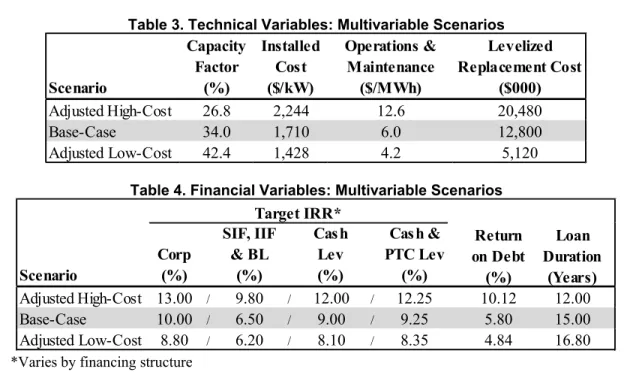
Analysts also modeled high-cost and low-cost multivariable scenarios to estimate the combined impact of varying all tested variables (technical and financial) simultaneously on the projected LCOE. However, the input parameters’ highest- and lowest-cost values are distinct from the values used in the individual variable sensitivities. The analysis adjusted the input parameters’ high- and low-cost values of the input parameters to be closer to the base case; this allowed analysts to model realistic and potentially achievable project characteristics when tested simultaneously. In other words, it is unlikely that any one project would have all of the most favorable (i.e., extreme low-cost) or least favorable (i.e., extreme high-cost) values together – some mix is likely more realistic. Table 3 illustrates the multivariable scenarios for the technical variables. Similarly, Table 4 illustrates the multivariable scenarios for the financial variables. Appendix B describes the methodology for determining these input values.

Table 3. Technical Variables: Multivariable Scenarios

Scenario Capacity Factor (%) Installed Cost ($/kW) Operations & Maintenance ($/MWh) Levelized Replacement Cost ($000) Adjusted High-Cost 26.8 2,244 12.6 20,480 Base-Case 34.0 1,710 6.0 12,800 Adjusted Low-Cost 42.4 1,428 4.2 5,120

Table 4. Financial Variables: Multivariable Scenarios

Scenario Corp (%) SIF, IIF & BL (%) Cash Lev (%) Cash & PTC Lev (%) Adjusted High-Cost 13.00 / 9.80 / 12.00 / 12.25 10.12 12.00 Base-Case 10.00 / 6.50 / 9.00 / 9.25 5.80 15.00 Adjusted Low-Cost 8.80 / 6.20 / 8.10 / 8.35 4.84 16.80 Target IRR* Return on Debt (%) Loan Duration (Years)

4.3 Technical vs. Financial Multivariable Scenario Analysis

Analysts examined a final scenario that divided the multivariable scenario analysis into two subgroupings. They tested technical variables (capacity factor, installed cost, O&M, and

levelized replacement cost) separately from financing variables (target IRR, return on debt, and loan duration). The LCOE was estimated with the technical variables set to their respective adjusted high-cost (or low-cost) multivariable scenario values while the financial variables were fixed to their base-case values and then vice versa. Analysts performed this test to see which subset of variables had a larger impact on the estimated LCOE.

(15)

7

5 Results

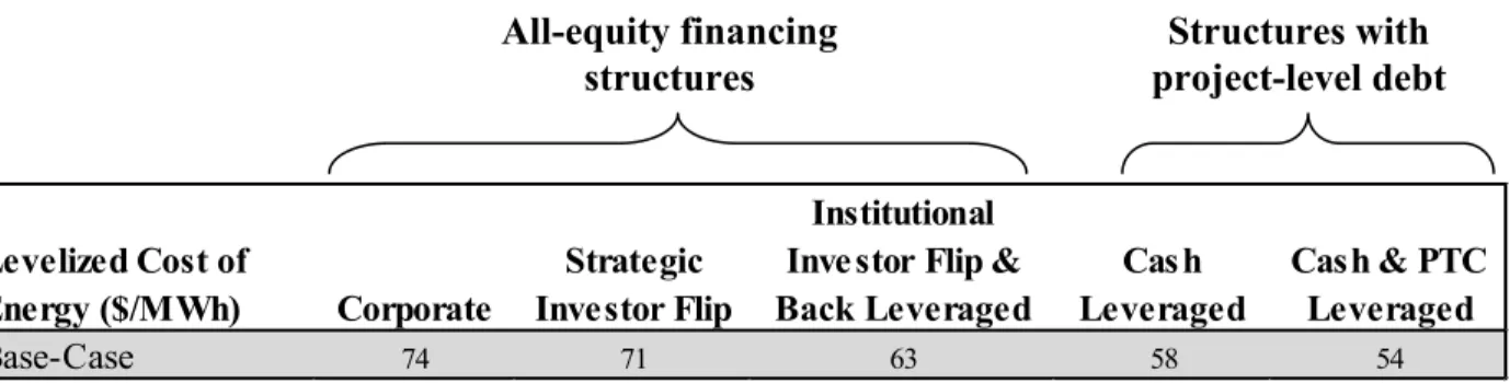
Table 5 shows the base-case LCOE estimates from the individual variable sensitivities, based on financial structure. The base-case LCOE provides a baseline measure to compare results from the sensitivity and scenario analyses that follow.8

Table 5. Base-Case LCOE Estimates

Levelized Cost of

Energy ($/MWh) Corporate Investor FlipStrategic

Institutional Investor Flip &

Back Leveraged LeveragedCash Cash & PTC Leveraged

Base-Case 74 71 63 58 54

5.1 Individual Variable Sensitivities

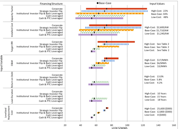
Figure 1 shows the resulting range of estimated LCOE for the individual variable sensitivities, which plots each variable’s highest- and lowest-cost input values for all of the financing

structures tested. The input variables in Figure 1 are ordered according to impact on the LCOE, from largest impact to smallest (top to bottom). The input parameters with the largest variation between the highest- and lowest-cost LCOE estimates generally have the greatest impact on overall wind project costs. Appendix C lists the complete results of the individual variable

sensitivity analysis, including all interim tested values between the highest- and lowest-cost input parameters.

8_{Again, note that for these analyses, the Institutional Investor Flip and Back-Leveraged financing structure are} identical at the project level (Back-Leveraged structure uses corporate-level debt, which is not captured in the model) and, therefore, return identical results.

All-equity financing

(16)

8

20 40 60 80 100 120 140 160

Cash & PTC LeveragedCash Leveraged Institutional Investor Flip & Back LeveragedStrategic Investor Flip Corporate Cash & PTC LeveragedCash Leveraged Institutional Investor Flip & Back LeveragedStrategic Investor Flip Corporate Cash & PTC LeveragedCash Leveraged Institutional Investor Flip & Back LeveragedStrategic Investor Flip Corporate Cash & PTC LeveragedCash Leveraged Institutional Investor Flip & Back LeveragedStrategic Investor Flip Corporate Cash & PTC LeveragedCash Leveraged Institutional Investor Flip & Back LeveragedStrategic Investor Flip Corporate Cash & PTC LeveragedCash Leveraged Institutional Investor Flip & Back LeveragedStrategic Investor Flip Corporate Cash & PTC LeveragedCash Leveraged Institutional Investor Flip & Back LeveragedStrategic Investor Flip Corporate -Le ve liz ed Re pl ac em en t Co st Lo an D ur at io n Re tur n o n D ebt O &M Ta rg et I RR In st al le d C ost Ca pac ity F ac to r LCOE $/MWh Input V ar ia bl e Base-Case

Financing Structure Input Values

High-Cost: 22% Base-Case: 34% Low-Cost: 48% High-Cost: 25,600 ($000) Base-Case: 12,800 ($000) Low-Cost: 0 ($000) High-Cost: 10 Years Base-Case: 15 Years Low-Cost: 18 Years High-Cost: 13.0% Base-Case: 5.8% Low-Cost: 4.2% High-Cost: $17/MWh Base-Case: $6/MWh Low-Cost: $3/MWh High-Cost: See Table 2 Base-Case: See Table 2 Low-Cost: See Table 2 High-Cost: $2,600/kW Base-Case: $1,710/kW Low-Cost: $1,240/kW

Figure 1. LCOE ranges by individual variable sensitivities, showing all financing structures The results of the individual variable sensitivity analysis indicate that among the input parameters tested, capacity factor and installed cost have the largest impact on the estimated LCOE. Target IRR has the largest impact among the financing variables tested, particularly for financing structures that use 100% equity. O&M costs had a moderate impact on the LCOE. For the financing structures that use debt at the project level (Cash Leveraged and Cash and PTC Leveraged), the loan terms have a modest effect on LCOE. The levelized replacement cost has the lowest impact on projected LCOE.

The relative impacts of each input variable on the projected LCOE are depicted in greater detail in Figures 2 and 3 and in Appendix C (Figures C1-C3 are included in Appendix C, because the results are similar to those in the figures presented here). Each figure illustrates a different financing structure tested.

In Figures 2 and 3, the percentage change of the input variable from the base case is shown along the X-axis. The two Y-axes show the resulting estimated LCOE that corresponded with the change in the input variable in percentage terms (from the base case) as well as in dollars per megawatt-hour ($/MWh). For each input variable, the slope of the plotted line shows the

(17)

9

variable’s impact on the LCOE. The steeper the slope, the greater the impact an input variable has on the LCOE.

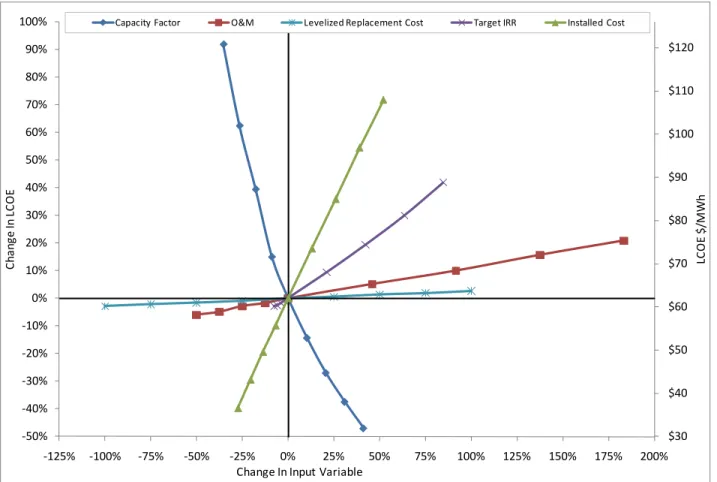
Figure 2 shows the LCOE sensitivity to the tested individual variables in the all-equity, Institutional Investor Flip financing structure. This structure represents the majority of third-party (non-corporate) financing deals from 2003-2006 (Harper et al. 2007). As shown, installed cost and capacity factor have the largest impact on LCOE, even though the ranges tested were relatively small (in percentage terms from the base-case input value).9

Target IRR also shows a large impact on the LCOE – an approximate 40% increase in the target IRR increases the estimated LCOE by around 20%.

$30 $40 $50 $60 $70 $80 $90 $100 $110 $120 -50% -40% -30% -20% -10% 0% 10% 20% 30% 40% 50% 60% 70% 80% 90% 100% -125% -100% -75% -50% -25% 0% 25% 50% 75% 100% 125% 150% 175% 200% LC O E $ /M Wh Cha ng e I n L CO E

Capacity Factor O&M Levelized Replacement Cost Target IRR Installed Cost

Change In Input Variable

Figure 2. Institutional Investor Flip LCOE sensitivities by input variable

9_{Installed cost, target IRR, O&M, return on debt, and levelized replacement cost are directly proportional to the} estimated LCOE. Capacity factor and loan duration (Figure 3) are inversely proportional.

(18)

10

Figure 3 shows the LCOE sensitivity to individual variables in the Cash Leveraged financing structure, which incorporates the use of debt financing. It shows that most of the variables have the same relative relationships as the Institutional Investor Flip financing structure (Figure 2). The exception is target IRR, which has about the same percentage change in input variable, but a significantly lower impact on LCOE. This makes sense due to the addition of debt, which reduces the portion of equity investment in the project from 100% to approximately 55%. The addition of debt also adds two new variables – the loan duration and return on debt (or interest rate), both of which appear to have moderate impacts on LCOE.

$30 $40 $50 $60 $70 $80 $90 $100 $110 -50% -40% -30% -20% -10% 0% 10% 20% 30% 40% 50% 60% 70% 80% 90% 100% -125% -100% -75% -50% -25% 0% 25% 50% 75% 100% 125% 150% 175% 200% LC O E $ /M Wh Cha ng e I n L CO E

Capacity Factor O&M Levelized Replacement Cost Target IRR Installed Cost Loan Duration

Return on Debt

Figure 3. Cash Leveraged structure LCOE sensitivities by input variable

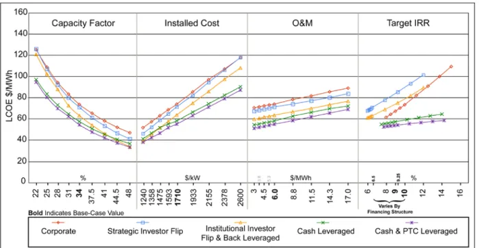
Figure 4 plots the most impactful input variables for all financing structures. The range of each variable’s tested values is plotted against the estimated LCOE.

The shapes of the curves are noteworthy. With the exception of the target IRR parameter, the overall slopes of the projected LCOE are similar among the six financing structures, which indicates that the impacts of the variables are fairly consistent across financing types. Installed cost and O&M appear to have a mostly linear relationship to the estimated LCOE. This suggests that reducing installation costs or O&M expenditures will have a fairly consistent impact on the LCOE. Capacity factor, on the other hand, has a dramatic impact on the LCOE for

below-average projects but levels somewhat as below-average or above-below-average capacity factors are achieved. This suggests that especially large reductions in LCOE can result from capacity factor

(19)

11

impact of the target IRR financing variable fluctuates by financing structure because each has a unique combination of equity capital investment and associated risk characteristics for the project investors.

The actual level ($/MWh) of the estimated LCOE varies by financing structure. The structures involving the use of debt (Cash Leveraged as well as Cash and PTC Leveraged) show lower estimated LCOEs compared to the all-equity financing structures. The Cash and PTC-Leveraged structure shows the lowest estimated LCOE because it uses the greatest percentage of debt financing, which is generally cheaper than equity financing (assuming debt interest rates are less than the equity target IRR).

Figure 4. LCOE sensitivities for capacity factor, installed cost, O&M, and target IRR by financing structure

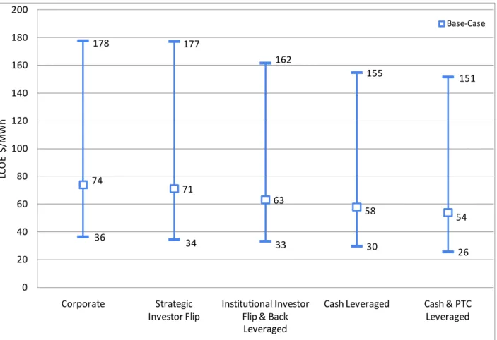
5.2 Multivariable Scenarios

The multivariable scenario analysis estimated the combined impact of varying an entire set of inputs simultaneously on the projected LCOE. Figure 5 shows the results of the multivariable- scenario analysis between the high-cost, base-case, and low-cost scenarios.

(20)

12 178 177 162 155 ₁₅₁ 36 ₃₄ 33 ₃₀ 26 74 71 63 58 ₅₄ 0 20 40 60 80 100 120 140 160 180 200 Corporate Strategic Investor Flip Institutional Investor Flip & Back Leveraged

Cash Leveraged Cash & PTC Leveraged LC O E $/M W h Base-Case

Figure 5. Multivariable scenarios LCOE ranges

Figure 5 shows the extent to which the estimated LCOE varies among optimal, average, and substandard wind projects. To put these LCOEs into context compared to electricity prices, it is important to know that the average wholesale power prices ranged regionally from about $45/MWh to more than $80/MWh in 2008 (Wiser and Bolinger 2009). Comparatively, the low-cost multivariable scenario is on the low end of that scale with an LCOE of $26-$36/MWh, depending on financing structure. This indicates that wind projects with superior resource attributes, low-cost equipment, and excellent financing terms can be cost-competitive with U.S. wholesale power prices.10_{The base-case scenario’s estimated LCOE range of $54-$74/MWh is} comparable to the range of wholesale power prices. The high-cost scenario has an estimated LCOE range of $151–$178/MWh, more than double wholesale power prices. As such, high-cost and poor-performing wind projects with higher financing terms are not directly competitive with wholesale power prices across most of the United States.

Because there is a wide range of site-specific costs and technology drivers for individual projects, it is difficult to make generalizations about LCOE for wind that hold true for wind projects, as a whole, across the nation. Therefore, site-specific considerations (size of project, economies of scale, resource quality, etc.) are critical when considering the cost of wind energy.

10_{This ignores the current financial uncertainties surrounding the financial crisis, the current limitations on access to} debt and equity, as well as increased competition among projects.

(21)

13

5.3 Technical- Versus Financial-Variable Scenarios

Figure 6 shows the results of varying the suite of technical and financial variables separately. The range of projected LCOE that results from varying the technical variables as a whole (and holding the financial variables constant) is illustrated in the lighter region, while the range of projected LCOE from varying the financial variables is shown in the darker region. Additionally, the base-case value for each structure is illustrated as a band within the LCOE ranges. As

anticipated from the individual variable results, varying the set of technical variables as a whole has a larger effect on the estimated LCOE than the set of financial variables. This result shows why it is critical that developers and utilities site and select wind projects at locations with excellent resources and technical cost characteristics before considering financing. These characteristics typically have a much larger impact than a project’s financing terms.

Furthermore, the impact of financing variables varies by the structure of financing, and the set of financial variables have their largest impact on the LCOE within the Cash Leveraged as well as the Cash and PTC Leveraged structures. To date, however, these debt-leveraged models have seen limited use in wind project funding despite being among the cheapest options available (assuming debt interest rates are less than the equity target IRR). The implication is that market players might be willing to accept slightly higher project costs to avoid the involvement of conservative project lenders. This choice to avoid cheaper sources of financing is less of an issue for the highest-quality wind projects because the production benefits far outweigh the financing savings. However, for moderate-quality wind projects, the savings from better-than-average financing terms can have more impact. The debt-leveraged structures – the cheapest structure of wind financing – would offer an opportunity for overall project cost reductions in the face of wind resource, technology, or installation conditions that are less than ideal.11

11_{And with the contraction of capital available for equity investment due to the financial crisis, project-level debt} might be needed to get all of the projects under development built.

(22)

14 0 20 40 60 80 100 120 140 160 180 Corporate Strategic Investor Flip

Institutional Investor Flip & Back Leveraged

Cash Leveraged Cash & PTC Leveraged

LC

O

E $

/M

Wh

Technical Variables LCOE Range Financial Variables LCOE Range Base-Case LCOE

Figure 6. Technical- vs. financial-variables scenario analysis

6 Conclusions

The results of the individual variable sensitivities suggest several insights. As expected, changes in a project’s capacity factor and installed cost have such a significant impact on the LCOE that small improvements through improved R&D or manufacturing improvements can yield major benefits. The most dramatic reductions in LCOE occurred for projects that had below-average wind resource quality and that had incremental improvements in capacity factor. This suggests that increasing the capacity factor from substandard values to average capacity-factor levels can achieve especially large reductions in LCOE.

A less obvious, yet moderate impact on the LCOE resulted from a change in the target IRR financing term. As previously noted, in the 100% equity financed Institutional Investor Flip structure, an approximate 40% increase in the target IRR increases the estimated LCOE by about 20%. This indicates that the target equity return could have a sizable effect on LCOE if the range of high- and low-cost values widens beyond historical industry practice, a likely outcome of the financial crisis (Schwabe et al. 2009).

The analysis also examined two subsets of the input variables to compare the overall impact of technical versus financial variables. For each financing structure tested, the impact of technical variables on the overall estimated LCOE was noticeably larger than that of the financing terms.

(23)

15

Because debt generally costs less than equity, the relative impacts of the financing variables were maximized under the two structures that incorporate debt financing (Cash Leveraged and Cash and PTC Leveraged structures). However, to date, the leveraged deals have been quite rare; but they could be an opportunity for some, albeit smaller, cost savings if other cost reductions in wind and technical characteristics are difficult to achieve.

The move away from debt financing may have resulted from the project team wanting to maintain some of the “upside potential” for themselves. Compared to equity investors, debt lenders usually have more stringent risk-mitigation requirements (e.g., require long-term

contracts, require creditworthy off-takers, etc.) and have priority rights on project assets. Prior to the financial crisis, these measures may have been seen as detrimental to project economics – locking-in energy prices over the life of the project means that the project cannot take advantage of any potential upward swings in market prices. However, the sources for capital investment – tax equity and debt – have shrunk under current market conditions. Depending on how quickly and thoroughly these markets recover, the use of debt might emerge as an increasingly prevalent way to securing project financing going forward.

7 Future Analysis

While conducting the research for this study, the analysts discovered some points of interest that may warrant further in-depth analysis. Potential topics include:

1) Inflation sensitivities. This seems to be especially appropriate given the uncertainty surrounding the current economic environment. It would be helpful to model the effect as an individual sensitivity parameter relative to the other input variables.

2) Utility ownership. Utilities can own wind projects and use the PTC (Cory et al. 2008). Following a 2008 clarification by the Internal Revenue Service (IRS), utilities can own between 51% and 99% of a project, and take the full value of the PTC over the life of the project (Mann 2008). Although this ownership structure has seen limited use, investor-owned utilities (IOUs) may decide to own more wind projects going forward. Due to their regulated rate of return, IOUs could develop wind projects using better financing terms than developers, particularly in today’s troubled market where equity returns are expected to increase substantially. Therefore, because this type of ownership was not considered in the current analysis and could become more relevant, it should be investigated going forward.

3) Financial crisis of 2008-2009 and select U.S. federal legislation. The scarcity of debt and equity financing in late 2008 and 2009 is likely to increase the costs of financing capital-intensive wind projects. It could be temporary, but sustained cost increases are certainly a possibility. Government officials have enacted new and unfamiliar programs in response to the crisis, which will likely alter the financing structures included in this analysis. While it is still too early to discern exact impacts of these exceptional market conditions on wind energy cost determinants, the financing terms or the structures themselves should be revisited.

(24)

16

References

Bolinger, M.; Harper, J.; Karcher, M. (2008). “A Review of Wind Project Financing Structures in the USA,” Wind Energy Journal. September.

Cory, K.; Coughlin, J.; Jenkin, T.; Pater, J.; Swezey, B. (2008). “Innovations in Wind and Solar PV Financing,” National Renewable Energy Laboratory technical report NREL/TP-670-42919,

Februar

Hand, M. (2009). Personal interview with Maureen Hand, National Renewable Energy Laboratory in January 2009.

Harper, J.; Karcher, M.; and Bolinger, M. (2007) “Wind Project Financing Structures: A Review & Comparative Analysis,” Lawrence Berkeley National Laboratory technical report

LBNL-63434, September

Inflationdata.com (2008). “Inflation Rates for Jan 2008 – Present.” Inflationdata.com Web site,

accessed December

IRS (2008). Internal Revenue Bulletin2008-21, Internal Revenue Service, U.S. Department of

the Treasury, October

Karcher, M. (2008). Wind Financing Structures Pro Forma Model. Deacon Harbor Financial.

Mann, L. (2008). “IRS Reinterpretation Will Benefit Utilities RE Investments,” North American Windpower, September 2008, pp. 72-73.

Schwabe, P.; Cory, K.; Newcomb, J. (2009). “Renewable Energy Project Financing: Impacts of the Financial Crisis and Federal Legislation,” National Renewable Energy Laboratory technical

report NREL/TP-6A2-44930, Jul

Stoel Rives (2009). Review of Pro Forma Wind Model. Memorandum from representatives of Stoel Rives LLP, March 25, 2009.

Wiser, R.; Bolinger, M. (2009). “2008 Wind Technologies Market Report,” U.S. Department of Energy, Office of Energy Efficiency and Renewable Energy, July.

Wiser, R.; Bolinger, M. (2008). “Annual Report on U.S. Wind Power Installation, Cost, and Performance Trends: 2007,” U.S. Department of Energy, Office of Energy Efficiency and

(25)

17

Appendix A. Equity and Debt-Financing Assumptions

Tables A1-A3 list the assumptions used in the Harper et al. 2007 analysis and identify assumptions that were updated for this analysis. Table A1 details the assumptions that are common across all financing structures that were tested; Table A2 details the structure-specific assumptions in the equity-based financing structures; and Table A3 lists the assumptions for the structures that incorporate debt financing only.

Specifically, base-case assumptions updated from the Harper et al. 2007 analysis include: 1) Average installed wind project size was set at 120 MW to be consistent with the

average installed wind project size in 2007 (Wiser and Bolinger 2008).

2) Capacity factor is assumed at 34%, because the weighted average capacity factor for projects installed in 2006-2007 was reported as 33%-35% (Wiser and Bolinger 2008). 3) Average installed capital cost of a wind project built in 2007 increased to $1,710/kW

(Wiser and Bolinger 2008). The increase of installed capital costs was allocated to wind turbines and balance of plant components equally.

4) 2008 PTC adjustment factor was updated to the actual 2008 reported value of 1.3854 (IRS 2008).

5) All-in annual interest rate (return on debt) was set at 5.8% to be consistent with an average long-term debt interest rate used to finance a wind project as of January 1, 2008. This rate was based on conversations with renewable energy industry attorneys (Stoel Rives 2009).

6) Inflation rate was set at 4%, which was the average monthly inflation rate in 2008 based on the consumer price index (Inflationdata.com 2008).

7) Levelized replacement cost was set at $12.8 million over the life of a 120 MW wind project, based on discussions with wind project developers and equipment manufacturers (Hand 2009).

(26)

18

Table A1. Input Assumptions Common to All Structures Assumption Harper et al. 2007 value Modification2008 Source/Note

Year of Initial Commercial Operation 2007 2008 The project becomes operational January 1st 2008. Project Capacity 100 MW 120 MW

Annual Net Capacity Factor 36.00% 34.00%

Inflation Rate 2.00% 4.00% Inflationdata.com 2008.

Interest on Reserves 2.00% 4.00% Set to be consistent with assumed inflation rate.

Hard Costs

Development Costs 5,000 Unchanged Wind Turbines 120,000 160,200 Balance of Plant 25,000 30,000 Interconnection 10,000 Unchanged

Soft Costs

Interest During Construction

Interest Rate 6.70% 5.80% Stoel Rives 2009. Construction Period 12 Months Unchanged

Construction Debt Closing Fee (% of debt amount)

Soft Cost Totals

Interest During Construction Calculation Unchanged Equity Closing Costs 400 Unchanged Developer Fee 3,500 Unchanged

Working Capital 1,000 Unchanged Harper et al. 2007. Contingency 8,000 10,260 5% of Hard Costs. Operations & Maintenance Costs

Fixed O&M ($/kW-yr) 11.50 Unchanged Harper et al. 2007. Variable O&M ($/MWh) 6.00 Unchanged Harper et al. 2007. PPA Letter of Credit (LOC)

LOC AMOUNT ($000) 5,000 Unchanged Annual LOC Rate 1.50% Unchanged

Insurance ($000-yr) 0 Unchanged Harper et al. 2007. PTC Base Year ($/MWh) 15.00 Unchanged

2007 Inflation Adjustment Factor 1.3433 N/A

2008 Inflation Adjustment Factor 1.3702 1.3854 Internal Revenue Service Notice 2008-48.

2008 PTC Rate ($/MWh) 21.00 Unchanged $15/MWh multiplied by 1.3854 & rounded to nearest integer. Years Available 10 Unchanged Harper et al. 2007.

State 6% Unchanged

Federal 35% Unchanged

Hard Costs

Development Costs Indirect Unchanged Wind Turbines

Balance of Plant

Interconnection Direct 20-yr SL Unchanged Soft Costs

Interest During Construction (IDC) Indirect Unchanged Debt Closing Costs (when debt is used) Direct 15-yr SL Unchanged Debt Closing Fee (when debt is used) Indirect Unchanged Debt Service Review

Equity Closing Costs Working Capital

Developer Fee Indirect Unchanged Contingency (5% of Hard Costs) Indirect Unchanged

Harper et al. 2007. Harper et al. 2007. Unchanged Unchanged Taxes Deprecation Allocation Harper et al. 2007. Harper et al. 2007. Harper et al. 2007. Harper et al. 2007.

Wiser and Bolinger 2008 ($1,710/kW in aggregate).

1.25%

Direct 5-yr MACRS

Non-Depreciable

Unchanged Project Information

Capital Costs ($000)

Annual Operating Expenses

PTC

Wiser and Bolinger 2008.

(27)

19

Table A2. Structure-Specific Equity-Financing Assumptions

Developer Tax Developer Tax Source

Equity Contributions

Corporate 100% N/A Unchanged Unchanged Harper et al. 2007.

Strategic Investor Flip Cash Leveraged Cash & PTC Leveraged Institutional Investor Flip Back Leveraged Cash Allocations

Pre-Flip Cash

Strategic Investor Flip Cash Leveraged Cash & PTC Leveraged Institutional Investor Flip Back Leveraged

Post-Flip Cash

Strategic Investor Flip Cash Leveraged Cash & PTC Leveraged Institutional Investor Flip Back Leveraged Tax Benefits Allocations

Pre-Flip Tax

Strategic Investor Flip Cash Leveraged Cash & PTC Leveraged Institutional Investor Flip Back Leveraged

Post-Flip Tax

Strategic Investor Flip Cash Leveraged Cash & PTC Leveraged Institutional Investor Flip Back Leveraged Harper et al. 2007. 1% 99% 0% 100% Unchanged Unchanged 1% 90% 10% Unchanged Unchanged Unchanged Unchanged 0% 100%

Assumption Harper et al. 2007 value 2008 Modification

1% 99% 40% 60% Unchanged Unchanged Unchanged 95% 5% Stoel Rives 2009. Harper et al. 2007. Stoel Rives 2009. Unchanged Unchanged 99% 90% 10% Harper et al. 2007. Partnership Allocations 1% 99% Harper et al. 2007. Harper et al. 2007. Harper et al. 2007. Unchanged

(28)

20

Table A3. Structure-Specific Debt-Financing Assumptions

Assumption Harper et al. 2007 value Modification2008 Source/Note

Cash Flow Debt

Debt Tenor (Years) 15 Unchanged Harper et al. 2007.

All-In Annual Interest Rate 6.70% 5.80% Stoel Rives 2009. Debt Service Coverage Ratio 1.45 Unchanged Harper et al. 2007.

PTC Debt

Debt Tenor (Years) 10 Unchanged Harper et al. 2007.

All-In Annual Interest Rate 6.70% 5.80% Same assumption as term debt. Debt Service Coverage Ratio 1.45 Unchanged Harper et al. 2007.

Debt Closing Costs 400 Unchanged Harper et al. 2007.

Total Debt Closing Fee Calculation Unchanged Harper et al. 2007. Debt Service Reserve Calculation Unchanged Harper et al. 2007. Annual Debt Agency Fee ($000 flat) 25 & 40 Unchanged Harper et al. 2007. Debt Tenor (Years) years in the base Calculation (5.5

case) Unchanged Harper et al. 2007.

All-In Annual Interest Rate 6.70% 5.80% Same assumption as term debt. Debt Service Coverage Ratio 1.45 Unchanged Harper et al. 2007.

TERM DEBT (project-level debt backed by cash flows or a pledge of PTCs)

Both “Cash Leveraged” and “Cash & PTC Leveraged” Structures

BACK LEVERAGE DEBT (debt secured by the developer, rather than by the project itself)

(29)

21

Appendix B. Input Values

The following tested input values, including interim points between the high-cost (low-cost) and the base case, were used in the individual variable sensitivity analysis.

Table B1. Technical Variables: Individual Variable Sensitivities

Scenario Capacity Factor (%) Installed Cost ($/kW) Operations & Maintenance ($/MWh) Levelized Replacement Cost ($000) High-Cost 22 2,600 17.00 25,600 25 2,378 14.25 22,400 28 2,155 11.50 19,200 31 1,933 8.75 16,000 Base-Case 34 1,710 6.00 12,800 38 1,593 5.25 9,600 41 1,475 4.50 6,400 45 1,358 3.75 3,200 Low-Cost 48 1,240 3.00 0

Table B2. Financial Variables: Individual Variable Sensitivities

Cost Corp (%) SIF, IIF & BL (%) Cash Lev (%) Cash & PTC Lev (%) High-Cost 15.00 / 12.00 / 14.00 / 14.25 13.00 10.00 13.75 / 10.63 / 12.75 / 13.00 11.20 11.25 12.50 / 9.25 / 11.50 / 11.75 9.40 12.50 11.25 / 7.88 / 10.25 / 10.50 7.60 13.75 Base-Case 10.00 / 6.50 / 9.00 / 9.25 5.80 15.00 9.50 / 6.38 / 8.63 / 8.88 5.40 15.75 9.00 / 6.25 / 8.25 / 8.50 5.00 16.50 8.50 / 6.13 / 7.88 / 8.13 4.60 17.25 Low-Cost 8.00 / 6.00 / 7.50 / 7.75 4.20 18.00 Target IRR* Return on Debt (%) Loan Duration (Years)

For the multivariable scenario analysis, the adjusted input values (see Table 3 and Table 4 in section 4.2) were calculated as a two-step process. First, the delta between the input variable’s highest- (lowest-) cost value used in the individual sensitivities and its base-case value was derated by 0.6 (e.g. 60%). The derate was based on judgment of realistic project assumptions. As previously mentioned, it is unlikely that any particular wind project would have all the best technology and financial assumptions (or worst) at the same time. Rather it is more likely that a single project would have a more modest set of variables together, hence the presumed derate. Second, the resulting reduced delta was added (subtracted) to the base-case value to give the input variable’s highest- (lowest-) cost value for the multivariable sensitivity analysis. This was repeated for all variables.

(30)

22

Appendix C. Additional Results

Table C1. LCOE Results:12 Input

Variable AdjustmentsSensitivity ($/MWh)LCOE Base-CaseΔ From ($/MWh)LCOE Base-CaseΔ From ($/MWh)LCOE Base-CaseΔ From ($/MWh)LCOE Base-CaseΔ From ($/MWh)LCOE Base-CaseΔ From

22.0% 125 70% 126 77% 121 92% 97 69% 95 74% 25.0% 109 48% 107 51% 102 62% 84 45% 80 48% 28.0% 94 28% 92 30% 88 39% 73 27% 70 28% 31.0% 83 13% 80 13% 72 15% 64 12% 62 15% 34.0% 74 0% 71 0% 63 0% 58 0% 54 0% 37.5% 65 -11% 61 -14% 54 -14% 51 -12% 47 -13% 41.0% 58 -21% 53 -25% 46 -27% 45 -21% 42 -23% 44.5% 52 -29% 47 -34% 39 -38% 41 -30% 37 -31% 48.0% 47 -36% 41 -42% 33 -47% 37 -37% 33 -39% $2,600/kW 118 61% 119 67% 108 72% 90 57% 87 60% $2,377.5/kW 107 46% 106 50% 98 55% 82 43% 79 45% $2,155/kW 97 32% 94 33% 86 36% 74 28% 71 30% $1,932.5/kW 85 16% 82 16% 74 18% 66 14% 62 15% $1,710/kW 74 0% 71 0% 63 0% 58 0% 54 0% $1,592.5/kW 68 -7% 64 -9% 57 -10% 54 -5% 51 -6% $1,475/kW 62 -15% 58 -18% 51 -19% 51 -12% 46 -16% $1,357.5/kW 57 -23% 51 -28% 45 -29% 46 -21% 41 -24% $1,240/kW 51 -31% 45 -36% 38 -40% 40 -30% 37 -32% See Table B2 110 49% 102 43% 90 42% 65 12% 59 8% See Table B2 100 36% 94 32% 82 30% 63 10% 58 6% See Table B2 91 24% 86 21% 75 19% 61 7% 57 4% See Table B2 82 12% 78 10% 69 9% 59 3% 56 2% See Table B2 74 0% 71 0% 63 0% 58 0% 54 0% See Table B2 70 -4% 70 -2% 63 -1% 57 -1% 54 -1% See Table B2 67 -8% 69 -3% 62 -2% 56 -2% 53 -2% See Table B2 65 -12% 69 -3% 61 -3% 56 -3% 53 -2% See Table B2 62 -16% 68 -4% 61 -3% 55 -4% 53 -3% $17/MWh 89 21% 84 18% 76 21% 72 25% 69 26% $14.25/MWh 85 16% 80 12% 73 16% 69 20% 65 20% $11.5/MWh 81 11% 77 8% 69 10% 66 14% 61 13% $8.75/MWh 78 6% 74 4% 66 5% 62 8% 58 7% $6/MWh 74 0% 71 0% 63 0% 58 0% 54 0% $5.25/MWh 73 -1% 70 -2% 62 -2% 57 -2% 53 -2% $4.5/MWh 72 -2% 69 -3% 61 -3% 56 -3% 52 -4% $3.75/MWh 71 -4% 68 -4% 60 -5% 55 -5% 51 -5% $3/MWh 70 -5% 67 -6% 59 -6% 54 -6% 50 -7% 13.0% 76 32% 77 41% 11.2% 70 22% 71 31% 9.4% 66 15% 65 19% 7.6% 62 7% 59 9% 5.8% 58 0% 54 0% 5.4% 57 -1% 53 -2% 5.0% 56 -3% 52 -4% 4.6% 55 -4% 51 -6% 4.2% 54 -6% 50 -8% 10 Years 74 29% 67 24% 11.25 Years 70 21% 65 20% 12.5 Years 65 13% 61 12% 13.75 Years 62 7% 58 7% 15 Years 58 0% 54 0% 15.75 Years 57 -1% 54 -1% 16.5 Years 56 -3% 53 -2% 17.25 Years 55 -4% 51 -6% 18 Years 54 -6% 51 -6% 25,600 ($000) 76 3% 72 2% 65 3% 59 3% 56 3% 22,400 ($000) 75 2% 72 2% 64 2% 59 2% 56 2% 19,200 ($000) 75 2% 71 1% 64 1% 58 2% 55 2% 16,000 ($000) 74 1% 71 0% 63 1% 58 1% 55 1% 12,800 ($000) 74 0% 71 0% 63 0% 58 0% 54 0% 9,600 ($000) 73 0% 70 -1% 63 -1% 57 -1% 54 -1% 6,400 ($000) 73 -1% 70 -1% 62 -2% 57 -1% 54 -2% 3,200 ($000) 73 -1% 69 -2% 62 -2% 56 -2% 53 -2% 0 72 -2% 69 -2% 61 -3% 56 -3% 53 -3% O& M N/A Level ize d R ep lac em en t C ost Loa n D ur at ion R et ur n on D ebt Lar gest Im pact O n L C O E M od er at e I m pact O n L C O E Sm al lest Im pact O n LC OE C ap aci ty F act or In st al led C ost Tar get IR R N/A Cash & PTC Leveraged Strategic Investor Flip Institutional Investor Flip & Back

Leveraged Cash Leveraged

Corporate

Individual Variable Sensitivities

(31)

23 $35 $45 $55 $65 $75 $85 $95 $105 $115 $125 $135 $145 -50% -40% -30% -20% -10% 0% 10% 20% 30% 40% 50% 60% 70% 80% 90% 100% -125% -100% -75% -50% -25% 0% 25% 50% 75% 100% 125% 150% 175% 200% LC O E $ /M Wh Cha ng e I n L CO E

(32)

24 $35 $45 $55 $65 $75 $85 $95 $105 $115 $125 $135 -50% -40% -30% -20% -10% 0% 10% 20% 30% 40% 50% 60% 70% 80% 90% 100% -125% -100% -75% -50% -25% 0% 25% 50% 75% 100% 125% 150% 175% 200% LC O E $ /M Wh Cha ng e I n L CO E

(33)

25 $25 $35 $45 $55 $65 $75 $85 $95 $105 -50% -40% -30% -20% -10% 0% 10% 20% 30% 40% 50% 60% 70% 80% 90% 100% -125% -100% -75% -50% -25% 0% 25% 50% 75% 100% 125% 150% 175% 200% LC O E $ /M Wh Cha ng e I n L CO E

Capacity Factor O&M Levelized Replacement Cost Target IRR Loan Duration Return on Debt

Installed Cost

(34)

F1147-E(10/2008)

REPORT DOCUMENTATION PAGE _{OMB No. 0704-0188}Form Approved

The public reporting burden for this collection of information is estimated to average 1 hour per response, including the time for reviewing instructions, searching existing data sources, gathering and maintaining the data needed, and completing and reviewing the collection of information. Send comments regarding this burden estimate or any other aspect of this collection of information, including suggestions for reducing the burden, to Department of Defense, Executive Services and Communications Directorate (0704-0188). Respondents should be aware that notwithstanding any other provision of law, no person shall be subject to any penalty for failing to comply with a collection of information if it does not display a currently valid OMB control number.

PLEASE DO NOT RETURN YOUR FORM TO THE ABOVE ORGANIZATION. 1. REPORT DATE (DD-MM-YYYY)

October 2009 2. REPORT TYPETechnical Report 3. DATES COVERED (From - To)

4. TITLE AND SUBTITLE

Wind Levelized Cost of Energy: A Comparison of Technical and Financing Input Variables

5a. CONTRACT NUMBER

DE-AC36-08-GO28308

5b. GRANT NUMBER

5c. PROGRAM ELEMENT NUMBER 6. AUTHOR(S)

K. Cory and P. Schwabe 5d. PROJECT NUMBERNREL/TP-6A2-46671

5e. TASK NUMBER

WER9.3550

5f. WORK UNIT NUMBER 7. PERFORMING ORGANIZATION NAME(S) AND ADDRESS(ES)

National Renewable Energy Laboratory 1617 Cole Blvd.

Golden, CO 80401-3393

8. PERFORMING ORGANIZATION REPORT NUMBER

NREL/TP-6A2-46671

9. SPONSORING/MONITORING AGENCY NAME(S) AND ADDRESS(ES) 10. SPONSOR/MONITOR'S ACRONYM(S)

NREL

11. SPONSORING/MONITORING AGENCY REPORT NUMBER 12. DISTRIBUTION AVAILABILITY STATEMENT

National Technical Information Service U.S. Department of Commerce

5285 Port Royal Road Springfield, VA 22161

13. SUPPLEMENTARY NOTES 14. ABSTRACT (Maximum 200 Words)

The expansion of wind power capacity in the United States has increased the demand for project development capital. In response, innovative approaches to financing wind projects have emerged and are proliferating in the U.S. renewable energy marketplace. Wind power developers and financiers have become more efficient and creative in structuring their financial relationships, and often tailor them to different investor types and objectives. As a result, two similar projects may use very different cash flows and financing arrangements, which can significantly vary the economic

competitiveness of wind projects. This report assesses the relative impact of numerous financing, technical, and operating variables on the levelized cost of e (LCOE) associated with a wind project under various financing structures in the U.S. marketplace. Under this analysis, the impacts of several financial and technical variables on the cost of wind electricity generation are first examined individually to better understand the relative importance of each. Then,analysts examine a low-cost and a high-cost financing scenario, where multiple variables are modified

simultaneously. Lastly, the analysis also considers the impact of a suite of financial variables versus a suite of technical variables.

nergy

15. SUBJECT TERMS

levelized cost of energy; LCOE; NREL; analysis; wind energy; wind project; wind financing; wind developers; wind markets; technical variables; wind modeling; production tax credit; Paul Schwabe; Karlynn Cory

16. SECURITY CLASSIFICATION OF: 17. LIMITATION OF ABSTRACT

UL

18. NUMBER

OF PAGES 19a. NAME OF RESPONSIBLE PERSON a. REPORT

Unclassified b. ABSTRACT Unclassified c. THIS PAGE Unclassified _{19b. TELEPHONE NUMBER}₍_{Include area code)}

Standard Form 298 (Rev. 8/98)