NBER WORKING PAPER SERIES
THE EXPECTED VALUE PREMIUM Long Chen
Ralitsa Petkova Lu Zhang Working Paper 12183
http://www.nber.org/papers/w12183
NATIONAL BUREAU OF ECONOMIC RESEARCH 1050 Massachusetts Avenue
Cambridge, MA 02138 April 2006
Chen: Department of Finance, Eli Broad College of Business, Michigan State University, 327 Eppley Center, East Lansing, MI 48823; tel: (517)353-2955, fax: (517)432-1080, email: [email protected]. Petkova: Department of Banking and Finance, Weatherhead School of Management, Case Western Reserve University, 10900 Euclid Avenue, Cleveland OH 44106; tel: (216)368-8553, email: [email protected]. Zhang: Carol Simon Hall 3-160B, Simon School of Business, University of Rochester, 500 Wilson Boulevard, Rochester, NY 14627; tel: (585)275-3491, fax: (585)273-1140, email: [email protected]. We acknowledge helpful comments from Denitza Gintcheva and seminar participants at Kent State University and Case Western Reserve University. The views expressed herein are those of the author(s) and do not necessarily reflect the views of the National Bureau of Economic Research. ©2006 by Long Chen, Ralitsa Petkova and Lu Zhang. All rights reserved. Short sections of text, not to exceed two paragraphs, may be quoted without explicit permission provided that full credit, including ©
The Expected Value Premium
Long Chen, Ralitsa Petkova and Lu Zhang NBER Working Paper No. 12183
April 2006 JEL No. G1
ABSTRACT
Fama and French (2002) estimate the equity premium using dividend growth rates to measure the expected rate of capital gain. We use similar methods to study the value premium. From 1941 to 2002, the expected HML return is on average 5.1% per annum, consisting of an expected-dividend-growth component of 3.5% and an expected-dividend-to-price component of 1.6%. The ex-ante HML return is also countercyclical: a positive, one-standard-deviation shock to real consumption growth rate lowers this premium by about 0.45%. Unlike the equity premium, there is only mixed evidence suggesting that the value premium has declined over time.
Long Chen
321 Eppley Center
The Eli Broad College of Business Michigan State University
East Lansing, MI 48824 [email protected] Ralitsa Petkova
Weatherhead School of Management Case Western Reserve University 10900 Euclid Avenue
Cleveland, OH 44106 [email protected] Lu Zhang
William E. Simon Graduate School of Business Administration
University of Rochester Rochester, NY 14627 and NBER
1
Introduction
Value stocks (stocks with high book-to-market ratios) earn higher average returns than growth stocks (stocks with low book-to-market ratios). (See, for example, Graham and Dodd 1934; Rosenberg, Reid, and Lanstein 1985; Fama and French 1992; Lakonishok, Shleifer, and Vishny 1994). We study the value premium—the difference between the expected returns of value stocks and growth stocks—from a fresh angle by constructing an ex-ante measure of the value premium from cash flow fundamentals.
Our economic question is important. Following the seminal contributions of Fama and French (1992, 1993, 1996), the value premium has become arguably as important as the equity premium in portfolio allocation decisions, estimation of the cost of capital, and many other applications. Moreover, most previous studies use average realized returns as proxies for expected returns. But as expected-return proxies, average returns are extremely noisy (e.g., Elton, 1999; Fama and French, 2002). Specifically, the average return might not con-verge to the expected return in finite samples. As pointed out by Elton, there are periods longer than ten years during which the stock market return is on average lower than the risk free rate (1973–1984), and periods longer than 50 years during which risky bonds underper-form on average the risk free rate (1927–1981). Fama and French also argue forcefully that the estimates of expected returns from fundamentals, especially those from dividend growth are more precise and have lower standard errors than the estimates from the average returns. Our estimation methods follow Blanchard (1993) and Fama and French (2002). The idea is simple. A rearrangement of the Gordon growth model says that:
R = D
where R is the equity return, D
P is the dividend-to-price ratio, andg is the dividend growth
rate. From equation (1), the expected return can be decomposed into the expected dividend-to-price ratio and the expected dividend growth. To estimate these two components for value and growth portfolios, we regress their future dividend-price ratios and future dividend growth rates onto a set of conditioning variables. The expected value premium can then be calculated as the expected return of the value portfolio minus that of the growth portfolio.
Our ex-ante perspective provides fresh insights into the magnitude and components of the value premium. First, the expected HML return is on average 5.1% per annum from 1941 to 2002, consisting of an dividend-growth component of 3.5% and an expected-dividend-to-price component of 1.6%. The results are similar for the 1963–2002 subsam-ple: the expected HML return is on average 5.1% per annum with an expected-dividend-growth component of 2.8% and an expected-dividend-to-price component of 2.3%. Some-what surprisingly, a large portion of the value premium comes from the expected-dividend-growth component. This component is even more important in magnitude than the expected dividend-to-price component. This evidence suggests that cash flow fundamentals are more important than mean-reverting valuation ratios in driving the value premium.
Intriguingly, this result does not contradict the conventional wisdom that growth firms have more growth options and grow faster than value firms. The crux is that our evidence is obtained from portfolios rebalanced annually as in the Fama and French (1993) portfolio approach, while the conventional wisdom is based on portfolios with fixed sets of firms without rebalancing as in the event-study approach. Using the event-study approach as in Fama and French (1995), we document that growth stocks have higher real dividend growth rates than value stocks for ten years around the year of portfolio formation. For
example, from the double, 2×3 sort on size and book-to-market, the spread in real dividend growth between the small-growth and the small-value portfolio is about 15% at the portfolio formation year. However, with annual rebalancing, the firms in the growth portfolio next year are not the same as those in the portfolio this year. Because growth rates are measured using different sets of firms, there is no particular reason to expect the dividend growth of the growth portfolio to be higher than the dividend growth of the value portfolio.
And the expected value premium is countercyclical. From 1941 to 2002, the correlation between the expected HML return and the default spread, a well-known countercyclical vari-able, is 0.39 with a p-value of 0.00. The correlation between the expected HML return and the growth rate of real investment, a well-known procyclical variable, is−0.28 with ap-value of 0.03. The results are similar for the sample from 1963 to 2002. Moreover, the expected value premium responds negatively to positive shocks to real consumption growth and real investment growth rates. A positive one-standard-deviation shock to real investment growth lowers the expected HML return by 0.25–0.30% per annum. And a positive one-standard-deviation shock to real consumption growth lowers the expected HML return by 0.45–0.50% per annum. The link between the expected value premium and macroeconomic variables lends support to the risk-based interpretation of the value premium.
Finally, purged from its countercyclical fluctuations, the expected value premium exhibits a downward trend to some extent. But the evidence is somewhat mixed. Schwert (2003) shows that the magnitude of the value premium has declined in the 1990s following the publi-cation of Fama and French (1992, 1993), and argues that academic research has made capital markets more efficient. Our evidence lends some support to this argument. More generally, however, our evidence suggests that the reversion in profitability of the value strategies in
the 1990s is more likely to be driven by the countercyclicality of the expected value premium rather than by a more permanent downward trend.
Our paper adds to the growing literature that uses valuation models to estimate expected returns (e.g., Claus and Thomas 2000; Gebhardt, Lee, and Swaminathan 2000; Campello, Chen, and Zhang 2005). Our methods follow those in Blanchard (1993) and Fama and French (2002), who study the properties of the equity premium. We differ from all these papers because we focus exclusively on the value premium. Our analysis is also connected to Fama and French (2005), who break average value-minus-growth returns into dividends and three sources of capital gain including reinvestment of earnings, convergence in market-to-book ratios and general upward drift in market-to-market-to-book. We simply use long-term dividend growth to measure the rate of capital gain.
Our story proceeds as follows. Section 2 describes our estimation methods. Section 3 documents descriptive statistics for the ex ante value premium and its two components, the expected dividend-to-price ratio and the expected dividend growth rate. Section 4 studies the trend and cyclical properties of the premium. Section 5 deals with a variety of remaining issues. Finally, Section 6 summarizes and interprets our results.
2
Research Design
Section 2.1 discusses the basic idea underlying our methods, and Section 2.2 presents details of our sample construction.
2.1
The Basic Idea
We follow Blanchard (1993) and Fama and French (2002) to construct expected returns. The basic idea is simple. We estimate expected rates of dividend growth and expected
dividend-to-price ratios, and then combine them to obtain expected returns.
To be precise, let Rt+1 be the realized stock return from time t to t+1, i.e., 1+Rt+1=
(Dt+1+Pt+1)/Pt, where Pt is the stock price known at time t, and Dt+1 is the real dividend
paid over the period from t tot+1; Dt+1 is unknown until the beginning of time t+1. If we
assume that the dividend-to-price ratio is stationary, we can solve forPt as the present value
of future dividends discounted by the sequence of realized rates of return. As in Blanchard (1993), we next divide both sides byDt, take conditional expectations at timet, and linearize
to obtain the expected return at time t, denoted Et[Rt+1], as:
Et[Rt+1] = Et Dt+1 Pt + Et[Agt+1], (2)
where Agt+1 is the long-run growth rate of dividends defined as the annuity value of the
growth rate of future dividends
Agt+1 ≡ ¯ r−¯g 1 + ¯r ∞ X i=0 1 + ¯g 1 + ¯r i gt+i+1, (3)
with ¯gand ¯rbeing the average growth rate of real dividends and the average real stock return, respectively. Finally, gt+1 denotes the growth rate of real dividends from time t to t+1.
The interpretation of equation (2) is simple. Expected returns equal expected dividend-to-price ratios plus expected long-run dividend growth rates. And the expected value pre-mium equals the sum of the difference in the expected dividend-to-price ratios and the dif-ference in the expected long-run dividend growth rates between value and growth portfolios.
2.2
Estimation Details
We now discuss the details of estimating expected returns based on equations (2) and (3) for value and growth portfolios.
Sample Construction
We obtain relevant data from three main sources. The first source is the Center for Research in Securities Prices (CRSP) monthly stock file that contains information on stock prices, shares outstanding, dividends, and returns for NYSE, AMEX, and Nasdaq stocks. The second source is the COMPUSTAT annual research file that provides accounting information for publicly traded U.S. firms. To alleviate the potential survivorship bias due to backfilling data, we require that firms be on COMPUSTAT for two years before using the data. The third source is Moody’s book equity information used in Davis, Fama, and French (2000), available from Kenneth French’s web site at http://mba.tuck.dartmouth.edu/pages/faculty/ken.french/data-library.html.
Our sample goes from 1941 to 2002. In earlier periods, only a few firms have data on dividends once we classify them into value and growth portfolios. As discussed in Cohen, Polk, and Vuolteenaho (2003), potential problems with disclosure regulations also affect our choice of the starting date of the sample period.1
We construct value and growth portfolios by sorting on to-market ratios. We implement both a one-way sort to obtain five book-to-market quintiles and a two-way, two-by-three sort on size and book-book-to-market to obtain six portfolios following Fama and French (1993).
Our timing in portfolio construction differs slightly from that commonly used in the lit-erature. Instead of in June, we form portfolios in December of each year t. We use book equity from the fiscal year ending in calendar year t−1 divided by market equity at the end of December of year t. This method avoids any look-ahead bias that might arise because accounting information from the current fiscal year is often not available at the end of the 1Specifically, before the Securities Exchange Act of 1934, there was essentially no regulation to ensure
the flow of accurate and systematic accounting information. The act prescribes specific annual and periodic reporting and record keeping requirements for publicly traded companies.
calendar year. Portfolio ranking is effective from January of year t+1 to December of year
t+1. We choose this portfolio timing to facilitate the interpretation of our test results be-cause this timing is better in line with the timing of dividend growth which goes from the beginning to the end of the calendar year. Our different timing convention is not a source of concern, however. Using more lagged information on book value makes it harder for us to find an ex ante value premium. Moreover, using the more conventional timing as in Fama and French (1993) yields quantitatively similar results (not reported).
Our definition of book equity follows that of Cohen, Polk, and Vuolteenaho (2003). In particular, book equity is defined as the stockholder equity plus balance sheet deferred taxes (item 74) and investment tax credit (item 208 if available) plus post-retirement benefit liabilities (item 330 if available) minus the book value of preferred stock. Depending on data availability, we use redemption (item 56), liquidation (item 10), or par value (item 130), in this order, to represent the book value of preferred stock. Stockholders’ equity is equal to Moody’s book equity (whenever available) or the book value of common equity (item 60) plus the par value of preferred stock. If neither is available, the stockholder equity is calculated as the book value of assets (item 6) minus total liabilities (item 181).
Estimation
There are three basic steps in our estimation procedure.
First, for each portfolio, we construct the real dividend-to-price ratio from the time series of value-weighted realized stock returns with and without dividends and the time series of the consumer price index from the U.S. Bureau of Labor Statistics as follows:
Dt+1 Pt = Rt+1−R X t+1 CPIt CPIt+1 (4)
where Rt+1 is the nominal return with dividends from time t to t+1, RtX+1 is the nominal
return without dividends over the same period, and CPIt is the level of the consumer price
index. And we calculate the real dividend growth as:
gt+1 = Dt+1/Pt Dt/Pt−1 RX t + 1 CPIt−1 CPIt −1 (5)
The resulting real dividend growth rates are quite volatile even at the portfolio level. To control for the effects of the outliers, we replace any annual observations of dividend growth higher than 50% with 50% and those lower than −50% with −50%.
Second, we construct the long-run dividend growth rate, Agt+1, given by equation (3),
for each portfolio. Following Blanchard (1993), we estimate ¯r as the sample average of the realized real equity returns, and ¯g as the sample average of the real dividend growth rates.
Agt+1 is an infinite sum of future real dividend growth rates. In practice we use a finite sum
of 100 years of future growth. We assume that the future real dividend growth rates beyond 2002 equal the average dividend growth rate during the 1980–2002 period. We also use the full-sample average and find the results to be quite stable (not reported). The focus on the 1980–2002 period intends to pick up the more recent trend of dividend growth.
Third, we regress Agt+1 andDt+1/Pt on a set of conditioning variables. The fitted values
from these regressions provide the two components of the expected returns, and the sum of these components gives the time series of expected portfolio returns. The set of conditioning variables includes four aggregate variables and one portfolio-specific variable. Our choice of the four aggregate conditioning variables is standard from the time series predictability literature. These variables include: the aggregate dividend yield, computed as the sum of dividend payments accruing to the CRSP value-weighted portfolio over the previous 12
months, divided by the contemporaneous level of the index (e.g., Fama and French 1988); the default premium, defined as the yield spread between Moody’s Baa and Aaa corporate bonds from the monthly database of the Federal Reserve Bank of Saint Louis (e.g., Keim and Stambaugh 1986; Fama and French 1989); the term premium, defined as the yield spread between a long-term and a one-year Treasury bond from Ibbotson Associates (e.g., Campbell 1987; Fama and French 1989); and the one-month Treasury bill rate from CRSP (e.g., Fama and Schwert 1977; Fama 1981).
Previous studies find that the log market spread, defined as the log book-to-market of portfolio ten minus the log book-to-book-to-market of portfolio one from ten deciles sorted on book-to-market, can predict future value-minus-growth returns (e.g., Asness, Friedman, Krail, and Liew 2000; Cohen, Polk, and Vuolteenaho 2003). We therefore also use the log book-to-market spread to predict the long-run dividend growth rates and the dividend-to-price ratios of book-to-market portfolios. We obtain data on the returns and the year-end book-to-market ratios of all book-to-market deciles from Kenneth French’s web site. From January to December of year t, the book-to-market of a portfolio is calculated by dividing its book-to-market ratio at the end of December of year t−1, where book value and market value are both measured at the end of December, by its compounded gross return from the end of December of year t−1 to the current month of year t.
3
Descriptive Analysis
Our method is basically a dynamic version of the method used by Fama and French (2002) to compute the equity premium. Before we examine our results on the value premium, it is interesting to compare the properties of the equity premium constructed in our sample to those constructed by Fama and French.
3.1
The Equity Premium
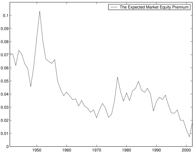
Our estimates on the equity premium are close to those from Fama and French (2002). During the 1951–2000 period studied by Fama and French, our estimates of the expected long-run real dividend growth rate, the expected real dividend yield, the expected real eq-uity market return, and the average realized real market return are 0.84%, 4.07%, 4.91%, and 10.21%, respectively. These values are fairly close to their counterparts, 1.05%, 3.70%, 4.75%, and 9.62%, respectively, reported by Fama and French. The differences are likely a result of our different sample construction. Consistent with Fama and French, the equity premium that we estimate is much lower than the average realized real equity return. The expected equity premium from 1941 to 2002 is 4.25% per annum, which is only about 55% of the realized real equity premium, 7.76% per annum, for the same sample period.
More important, our estimates show that the equity premium has declined over time, again consistent with Fama and French (2002). Figure 1 shows that the equity premium reaches its peak of about 10% in the early 1950s, declines over the next two decades to about 2.5% in the mid 1970s, climbs up to about 5% in the mid 1980s, then declines over the next one and half decades to about 1% in the early 2000s. Using the equity premium in a time-trend regression yields a negative slope of−0.077% per annum (t-statistic−8.46) in the 1941– 2002 sample. The slope is only an insignificant −0.021% (t-statistic −1.65) in the post-1963 sample, but it increases in magnitude to−0.142% (t-statistic−7.73) in the sample after 1980.
3.2
The Value Premium
Table 1 reports descriptive statistics for returns, dividend growth rates, dividend yields, both realized and expected, for value and growth portfolios. We report the results for the full sam-ple from 1941 to 2002 and the subsamsam-ple from 1963 to 2002. When we use the one-way sort
on book-to-market, we denote the resulting five portfolios as Low, 2, 3, 4, and High. Port-folios Low and High represent the two extremes. The difference between the returns of High and Low, denoted p5-1, represents the value-minus-growth strategy for the one-way sort. We denote the six portfolios from the two-way sort on size and book-to-market as S/L, B/L, S/M, B/M, S/H, and B/H. For example, portfolio S/L contains stocks with the bottom 30% book-to-market ratios and the bottom 50% market capitalizations. The value-minus-growth strategy for the two-way sort, denoted HML, is defined as (S/H + B/H)/2−(S/L + B/L)/2.
Average Returns
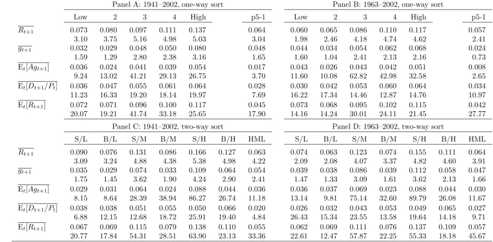
The first two rows of all panels in Table 1 show that value-minus-growth strategies are profitable in our samples. The average realized return of portfolio p5-1 is 5.8% per year (t-statistic 2.72) in the full sample, and 4.6% per year (t-statistic 1.94) in the subsample. Similarly, the average realized annual return of HML is 6% in the full sample and 5.9% in the subsample, and the t-statistics are 4.02 and 3.62, respectively.
Dividend Growth Rates
Rows three and four in all panels of Table 1 show that the realized real dividend growth rate of value portfolios is on average higher than that of growth portfolios, albeit the difference is mostly insignificant. For example, the real dividend growth rate,gt+1, of portfolio p5-1 is
on average 4.5% per annum in the full sample. Controlling for size increases the growth rate further to 5.6% for HML. And from the middle two rows of all panels, the expected long-run real dividend growth, Et[Agt+1], follows largely the same pattern. Except for p5-1 in the
subsample, the value portfolio has significantly higher expected long-run dividend growth than the growth portfolio. The average expected long-run dividend growth of HML is 3.5% per year in the full sample, and 2.8% in the subsample, and their t-statistics are 9.42 and
14.22, respectively, even after we control for heteroscedasticity and autocorrelations.
More important, our evidence does not contradict the conventional wisdom that growth stocks have higher proportions of growth opportunities and grow faster than value stocks. The reason is that our evidence is obtained from portfolios rebalanced annually, while the conventional wisdom is based on portfolios with fixed sets of firms without rebalancing.
To illustrate this point, we study the event-time evolution of profitability (defined as earnings divided by lagged book equity), the rate of dividend payment (defined as dividends divided by lagged book equity), and the real dividend growth rate for value and growth stocks for 21 years around the portfolio formation year. Our test design follows closely that of Fama and French (1995). We define value and growth portfolios both from book-to-market quintiles and from six size and book-to-market portfolios. As in any event studies, the stocks in the value and growth portfolios are held constant throughout the event years.
Our sample goes from 1941 to 2002. As explained in Section 2.2, we back out data on dividends from value-weighted portfolio returns with and without dividends. Because earnings data are not available in the pre-COMPUSTAT years, we follow Cohen, Polk, and Vuolteenaho (2003) and use the clean-surplus relation to compute earnings from data on book equity and dividends, i.e., earnings(t) =book value(t)−book value(t−1)+dividends(t). To be consistent, we use this method to compute earnings throughout our sample.
Figure 2 reports the results. First, Panels A and D confirm the main result in Fama and French (1995) that growth firms are persistently more profitable than value firms. Panels B and E show that growth firms also have higher rates of dividends than value firms. The spread in dividend rates appears even more persistent than the spread in profitability, especially for the two-way sort. This pattern is perhaps not surprising because firms are likely to be more
flexible in adjusting earnings through discretionary accruals than in adjusting dividends. More important, Panels C and F of Figure 2 show that the real dividend growth rates of growth stocks are higher than the real dividend growth rates of value stocks. For the one-way sort, the spread is about 10% at the portfolio formation year, and remains positive for almost ten years afterwards. For the two-way sort, the spread in dividend growth between the small-growth portfolio, S/L, and the small-value portfolio, S/H, is about 15% at the portfolio formation year, but the spread is much more short-lived and converges in about three years. However, when the portfolios are rebalanced annually, the firms in the growth portfolio next year are not the same as the firms in the growth portfolio this year. And there is no particular reason to expect the dividend growth of growth portfolios to be higher than the dividend growth of value portfolios because growth rates are measured using different sets of firms. Consistent with this observation, Figure 3 plots the time series of the annual realized real dividend growth rates for portfolios five and one in the book-to-market quintiles (Panel A), portfolio five-minus-one (Panel B), portfolios High and Low from the six portfolios sorted on size and book-to-market (Panel C), and HML (Panel D). From Panels B and D, the real dividend growth rates of growth portfolios are frequently lower than those of value portfolios.
Estimates for Expected Returns
The expected value premium is reliably positive in our sample. From the seventh and eighth rows in all panels of Table 1, the average expected dividend-to-price ratio, Et[Dt+1/Pt], is
higher for value firms than for growth firms. Because the expected long-run dividend growth rate and the expected dividend-to-price ratio are both higher for value firms, their expected returns are higher than the expected returns of growth firms. The last two rows of Panels A and B show that the expected return of p5-1 is 3.7% per year (t-statistic 7.74) in the full
sample, and 2.8% (t-statistic 7.74) in the subsample. Similarly, from the last two rows of Panels C and D, the expected HML return is 5.1% (t-statistic 27.80) in the full sample, and 5.1% (t-statistic 20.76) in the subsample.
From Table 1, the expected return for each portfolio in the one-way and two-way sorts is substantially lower than the average realized return of the portfolio. Previous studies have documented similar results for the market excess return. For example, Fama and French (2002) report that for the sample period 1951–2002 the expected equity premium is 4.32% per year, while the average realized equity premium is 7.43% per year. Fama and French conclude that average stock returns are a lot higher than expected. Our evidence suggests that this result also holds in the cross section of portfolios sorted by size and book-to-market. However, the expected value premium within each sorting procedure is not far away from the average realized return, suggesting that the difference between the expected return and the average realized return is similar in magnitude across value and growth portfolios.
Figure 4 plots the sample paths of the expected p5-1 return, the expected HML return, as well as their respective expected long-run dividend growth rates and expected dividend-to-price ratios. Panels A and C show that the expected p5-1 and HML returns are positive throughout the sample. Both series of expected returns display positive spikes during most of the recessions in the sample. The expected returns also covary positively with the default premium, a well-known countercyclical variable (e.g., Jagannathan and Wang 1996). This evidence suggests that the expected value premium is countercyclical.
From Panels B and D of Figure 4, there has been a noticeable decline in the expected long-run dividend growth from the early 1940s to the early 1980s, but an increase thereafter. The expected dividend-to-price ratios display the opposite long-term movements.
Accord-ingly, there is no obvious trend in the expected value premium, although the expected p5-1 return appears to decline slightly over time.
Predictive Regressions
We now report the predictive regressions used to construct the expected dividend growth and the expected dividend-to-price ratio, the two components of the expected value premium. Specifically, we regress the long-run dividend growth, Agt+1, and the dividend-to-price
ratio, Dt+1/Pt, on conditioning variables including the aggregate dividend yield, the default
premium, the term premium, the log book-to-market spread, and the one-month T-bill rate. We also regress the value premium defined as the sum ofAgt+1 and Dt+1/Pt on the same set
of conditioning variables. To adjust for the small-sample bias in the slopes and their standard errors (e.g., Stambaugh 1999), we use the simulation method of Nelson and Kim (1993).
These regressions are of independent interest. Previous studies (e.g., Asness, Friedman, Krail, and Liew 2000; Cohen, Polk, and Vuolteenaho 2003) document that the realized value premium is predictable using the log book-to-market spread, suggesting that the expected value premium is time-varying. Our analysis provides additional insights into this issue.
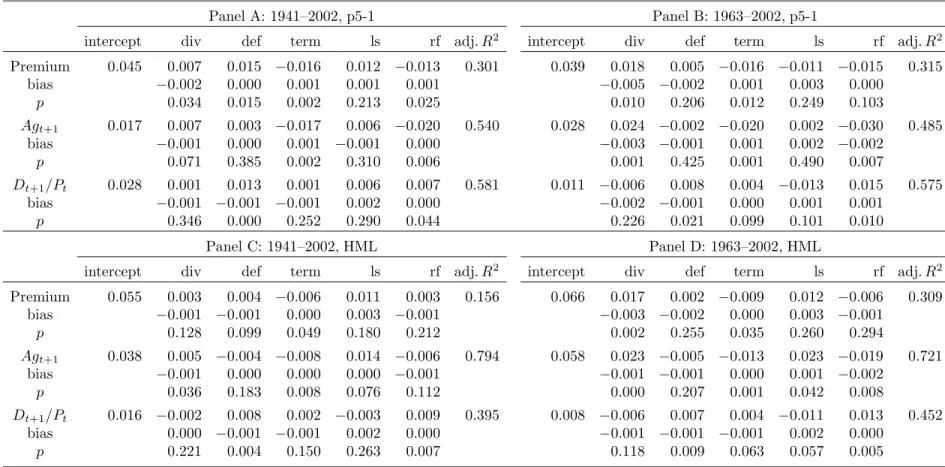
Table 2 reports the results. The first three rows of all panels show that the value premium is indeed predictable. The adjustedR2
clusters around 30% except for the HML return in the 1941–2002 sample that has an adjustedR2
of 15.60%. Although not reported in the table, the null hypothesis that all the slopes are jointly zero is strongly rejected in all cases. The results suggest that the aggregate dividend yield has reliable predictive power with positive slopes, except for the HML return in the period from 1941 to 2002. Further, the term premium has significant predictive ability for the expected value premium with negative slopes in all cases and across both sample periods. Panel B shows that, consistent with previous studies, we
find that the log book-to-market spread is largely a positive predictor of the value premium, except for predicting the p5-1 return in the post-1963 sample. However, our results also show that its predictive power is relatively weak because all corresponding p-values are close to 0.20. The default premium and the short-term rate do not have significant predictive ability for the expected value premium in the presence of the other conditioning variables.
The rest of Table 2 reports the results of predicting the two separate components of the value premium including the dividend growth rate and dividend-to-price ratio. These conditioning variables do an overall better job in predicting the separate components than the value premium itself. This is reflected in much higher adjusted R2
s; in some cases the goodness-of-fit coefficients are more than doubled.
We also study the robustness of our benchmark results with respect to alternative sets of instruments. We first exclude the log book-to-market spread from the list of conditioning variables. Alternatively, we include the cay and cdy variables from Lettau and Ludvigson (2001a, 2005) in the set of conditioning variables used to predict the dividend growth rates and the dividend-to-price ratios. In general, our results are largely unchanged. Details are not reported for brevity but are available upon request.
4
Dynamics of the Expected Value Premium
4.1
Trend Dynamics
There is some evidence for a downward trend in the low-frequency movements of the expected value premium, but the evidence is somewhat mixed. We use two methods to isolate the cyclical component of the expected value premium from the low-frequency, trend component.
The first method is to regress the expected value premium on a time trend:
Value Premiumt =a+b t+εt, (6)
where the fitted component including the intercept is defined as the trend component and the residual is defined as the cyclical component. The second method is to pass the expected value premium through the Hodrick-Prescott (1997) (HP) filter that separates the trend and the cyclical components of the premium.
The time-trend regressions suggest that the expected p5-1 return exhibits a downward trend in the 1941–2002 and the 1963–2002 samples, but the expected HML return does not. The expected HML return exhibits a slight downward trend in the 1980–2002 sample, but the expected p5-1 return does not. Specifically, the slope coefficient,b, is−0.078% per annum for the expected p5-1 return (t-statistic −8.01) in the 1941–2002 sample, −0.052% (t-statistic
−2.83) in the post-1963 sample, and −0.091% (t-statistic −1.86) in the 1980–2002 sample. The slope is−0.010% (t-statistic−1.47) for the expected HML return in 1941–2002,−0.011% (t-statistic −0.76) in 1963–2002, and −0.097% (t-statistic −3.12) in the 1980–2002 sample.
Panels A and B in Figure 5 plot the trend components of the expected p5-1 return and the expected HML return estimated from trend regressions and the HP-filter, respectively. Panel A shows a downward trend for p5-1 and but no clear trend for HML. Panel B shows a downward movement in the HP-filtered trend components for both p5-1 and HML.
4.2
Cyclical Dynamics
The expected value premium is countercyclical. We use two additional methods to study the cyclical properties of the expected value premium. As an informal test, we first report the lead-lag cross-correlation structure of the expected value premium with a list of cyclical
indicators. We then supplement the cross-correlations with a more formal VAR analysis.
Cross Correlations
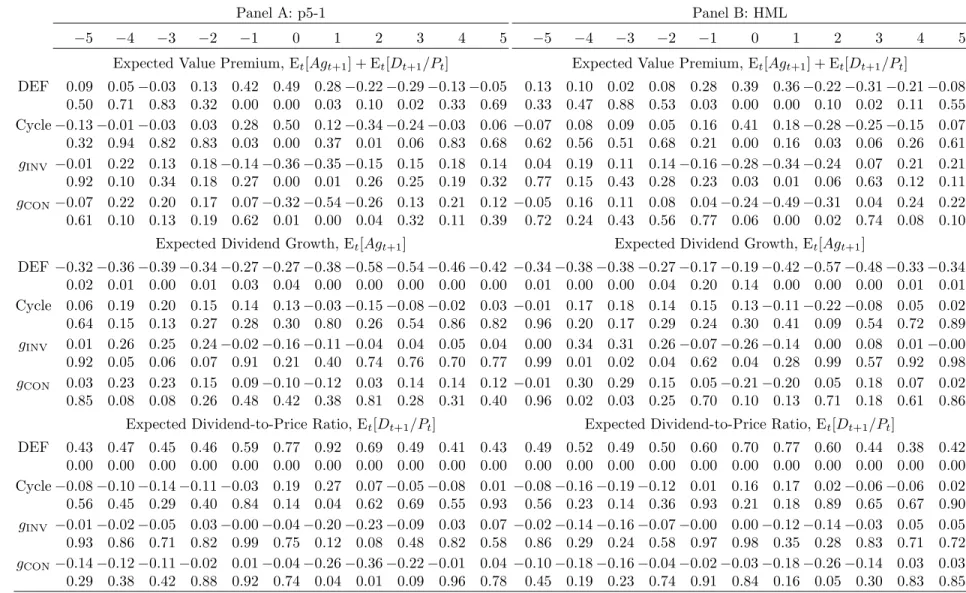
Table 3 reports the cross-correlations. The list of cyclical indicators includes the default pre-mium, the NBER recession dummy, the real investment growth rate, and the real consump-tion growth rate. Among the four variables, the default premium and the recession dummy are countercyclical, while the real investment and consumption growth rates are procyclical. From the middle column in Panel A of Table 3, the contemporaneous correlation between the expected 1 return and the default premium is 0.49 and that between the expected p5-1 return and the recession dummy is 0.50. Both are significant at the p5-1% level. Further, the contemporaneous correlation between the expected p5-1 return and real investment growth is −0.36 and that between the expected p5-1 return and real consumption growth is −0.32. The middle column in Panel B shows that using the expected HML return yields similar results. This evidence suggests that the expected value premium is countercyclical.
Panels C and D of Figure 5 plot the cyclical components of the expected p5-1 and HML return along with the NBER recession dummy. Panel C is based on the residuals from the time-trend regression, and Panel D is based on the HP filter. The expected p5-1 and HML returns peak in most recessions, suggesting that the premiums are countercyclical.
VAR Analysis
We next supplement the lead-lag correlations with a more formal VAR analysis. The VAR contains one measure of the expected value premium (either the expected p5-1 or the HML return) and one cyclical indicator. We use two cyclical variables separately in the VAR, the investment growth and the real consumption growth. Using other cyclical variables yields
largely similar results (not reported). The lag in the VAR is one, which is chosen according to the Akaike information criterion. In some specifications, we also include the one-month T-bill rate in the VAR to isolate real business cycle shocks from monetary policy shocks.
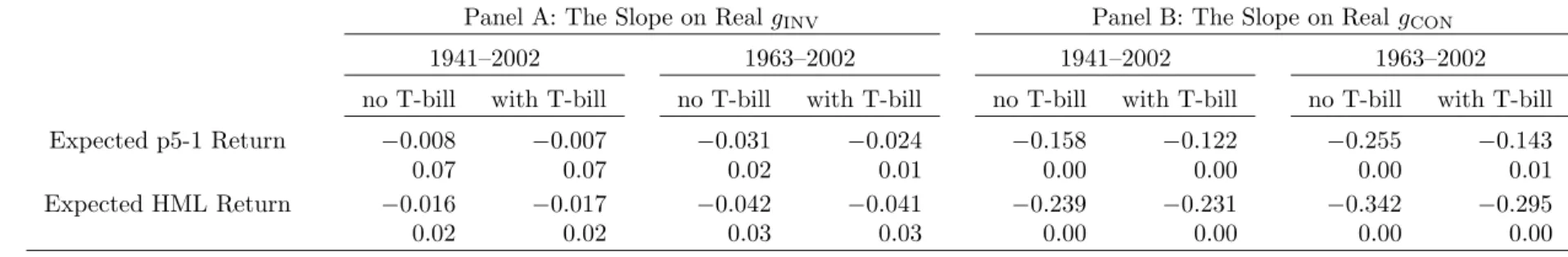
Table 4 reports the results. Panel A shows that the coefficients of real investment growth in the VAR are negative and mostly significant. This result holds with and without control-ling for the T-bill rate. Panel B shows that the coefficients of real consumption growth rate are all negative; they are all significant for both the long and the short sample periods. These results suggest that the expected value premium responds negatively to aggregate shocks.
To interpret the economic magnitudes of the VAR slopes, we study the impulse response functions from the estimated VARs. Panels A to D in Figure 6 plot the responses of the ex-pected value premium to a positive one-standard-deviation shock to real investment growth, and Panels E to H report the responses to a positive shock to real consumption growth. From Panels C and D, a positive one-standard-deviation shock to the real investment growth re-duces the expected HML return by 0.30% per annum without controlling for the T-bill rate and by about 0.26% with the T-bill rate. From Panels G and H, a positive one-standard-deviation shock to the real consumption growth reduces the expected HML return by 0.45% and 0.50% per annum with and without controlling for the T-bill rate, respectively. Using the expected p5-1 return yields similar results, although the magnitudes are somewhat lower. Our evidence on the countercyclical expected value premium lends support to the argu-ment that value stocks are riskier than growth stocks in bad times when the price of risk is high (e.g., Jagannathan and Wang 1996, Lettau and Ludvigson 2001b, Ang and Chen 2005; Petkova and Zhang 2005). Zhang (2005) provides a theoretical underpinning for this argu-ment. See also Lewellen and Nagel (2006) who, using short-window market regressions, find
little evidence that value-minus-growth betas covary positively with the expected market risk premium in the context of the conditional CAPM.
5
Incorporating Stock Repurchases
In this section, we redo all our tests after adding net stock repurchases as a part of total pay-out along with dividends. We find that incorporating stock repurchases increases the magni-tudes of the value premium; intuitively, value firms repurchase more shares than growth firms. The expected value premium continues to be countercyclical. And incorporating stock re-purchases further weakens the evidence on a downward trend in the expected value premium. Incorporating stock repurchases is important. Fama and French (2001) document that the proportion of firms paying cash dividends falls from 66.5% in 1978 to 20.8% in 1999. Moreover, firms have become less likely to pay dividends regardless of their characteristics. Grullon and Michaely (2002) also show that stock repurchases have become the dominant form of payout in recent years. Because of the importance of repurchases in total payout, it is necessary to evaluate its quantitative role in our measurement of the value premium.
To measure net stock repurchase, we follow Stephens and Weisbach (1998) in using the monthly decreases in shares outstanding as reported by CRSP adjusted for non-repurchasing activity affecting shares outstanding such as stock splits and dividend reinvestment plans. We also adjust for new stock issues following Jagannathan, Stephens, and Weisbach (2000). Let St denote the number of shares outstanding at month t and Pt denote the stock price.
IfSt−1> St, we define repurchase return as the decrease in value of shares outstanding from
month t−1 to t as a proportion of the market value of equity at month t−1. Formally:
Repurchase returnt−1,t =
(St−1−St)Pt−1 St−1Pt−1
We then add repurchase returns and stock returns with dividends together as stock returns with total payout. Finally, as in the benchmark estimation, we aggregate monthly returns into annual returns to avoid seasonality. And we back out payout growth rates from the difference between stock returns with total payout and rates of capital gain.
Table 5 reports the descriptive statistics for stock returns, dividend growth rates, and dividend-to-price ratios, both realized and expected, for value and growth portfolios. The value-minus-growth strategies are even more profitable after including stock repurchases. For example, the average realized return of portfolio p5-1 is 6.4% per annum in the full sample and 5.7% in the subsample, which are higher than 5.8% in the full sample and 4.6% in the subsample, respectively, in the benchmark case without repurchases. The realized returns of HML follow the same pattern. Including repurchases also increases the expected value premium. Specifically, the expected p5-1 return is on average 4.5% per annum in the full sample, higher than 3.7% in the benchmark case. The expected HML return goes up from 5.1% without repurchases to 5.5% with repurchases in the full sample. The results from the post-1963 sample are quantitatively similar. Finally, comparing Tables 1 and 5 reveals that the increase in the expected value premium from including repurchases is mostly derived from the expected-payout-to-price component. In particular, the expected-payout-growth component of the expected value premium is largely similar in magnitude to the expected-dividend-growth component in the benchmark estimation.
Panels A and B of Figure 7 plot the trend components of the expected p5-1 and HML returns after including stock repurchases. Based on time-trend regressions, Panel A shows a slight downward trend for p5-1, but a slight upward trend for the expected HML return. And from Panel B, there is no noticeable downward or upward trend in the HP-filtered,
low-frequency component of the expected HML return. The expected p5-1 return shows some dramatic decline in earlier periods, but remains relatively stable after the mid-1950s. Overall, a comparison between Figures 5 and 7 shows that the evidence suggesting a downward trend in the value premium is further weakened after including stock repurchases.
Turning to the cyclical properties of the value premium, Panels C and D of Figure 7 show that the countercyclicality of the value premium persists after we include stock repurchases. This informal evidence is further supplemented by Table 6 that reports the VAR results for the expected value premium with stock repurchases. From Panel A of the table, the slopes of real investment growth in the VARs are all negative and significant with and without controlling for the T-bill rates. And the magnitudes of the VAR coefficients are quantitatively very similar to those in the benchmark case reported in Table 4. Using real consumption growth yields largely similar results, as shown in Panel B. This evidence suggests that the expected value premium continues to respond negatively to aggregate shocks.
Finally, the impulse response functions reported in Figure 8 implied by the VAR analysis are again quantitatively similar to those reported in Figure 6 for the benchmark estimation. In all cases, the expected value premiums respond negatively to good news about real investment and consumption growth rates.
6
Summary and Interpretation
Fama and French (2002) estimate the equity premium using dividend growth rates to measure the expected rates of capital gain. We use similar methods to estimate ex-ante measures of the value premium from cash flow fundamentals.
From 1941 to 2002, the expected HML return is on average 5.10% per annum, consist-ing of an expected-dividend-growth component of 3.5% and an expected dividend-to-price component of 1.6%. Second, the expected value premium is countercyclical—a positive, one-standard-deviation shock to real consumption growth rate lowers the expected HML return by 0.45–0.50% per annum. Third, unlike the equity premium, there is only weak evidence suggesting that the value premium has declined over time. These basic findings are robust to a variety of perturbations in test design such as including stock repurchases into the cal-culations of cash flows, using alternative instrumental variables to estimate expected growth rates and expected dividend-to-price ratios, and using alternative portfolio constructions.
Our evidence contributes to our understanding of the driving forces behind the value premium. Three competing explanations coexist in the current literature. The first story says that the value premium results from rational variations of expected returns (e.g., Fama and French 1993, 1996; Lettau and Ludvigson 2001b). The second story argues that in-vestor sentiment causes the high premium for value stocks (e.g., De Bondt and Thaler 1985; Lakonishok, Shleifer, and Vishny 1994; Daniel, Hirshleifer, and Subrahmanyam 1998). The third story argues that the value premium results spuriously from sample-selection bias (e.g., Kothari, Shanken, and Sloan 1995; Schwert 2003) and data-snooping bias (e.g. MacKinlay 1995; Conrad, Cooper, and Kaul 2003).
We show that more than one half of the value premium is expected to come from the expected-dividend-growth component. This evidence lends direct support to Davis, Fama, and French (2000), who argue that the value premium is real and is unlikely to be driven purely by statistical biases. This interpretation is further buttressed by our large-sample evidence that there is no noticeable downward trend in the value premium. While largely
consistent with the evidence in Schwert (2003), our evidence suggests that the reversion in profitability of value strategies in the 1990s is more likely to reflect the countercyclicality of the expected value premium rather than a more permanent downward trend.
In addition, our evidence that the expected-dividend-growth component is higher in magnitude than the expected-dividend-to-price component in the composition of the value premium suggests that cash flow fundamentals, rather than mean-reverting valuation ratios, are more important driving forces behind the value premium. This evidence casts doubt on the overreaction story of De Bondt and Thaler (1985) and Lakonishok, Shleifer, and Vishny (1994) because this story works primarily through mispricing in valuation ratios and its slow correction in the long run, rather than cash flow fundamentals.
Finally, our evidence that the expected value premium is countercyclical lends support to the argument that value is riskier than growth in bad times when the price of risk is high (e.g., Jagannathan and Wang 1996; Lettau and Ludvigson 2001b; Ang and Chen 2005; Petkova and Zhang 2005; Zhang 2005). However, the magnitude of the negative response of the expected HML return to a positive, one-standard-deviation shock to real consumption growth rate is only about 0.50% per annum, which is less than one-tenth of the total magnitude of the value premium. This evidence lends support to the argument in Lewellen and Nagel (2006) that the role of conditioning information in driving the value premium is limited and that unconditional drivers are potentially more important (e.g., Fama and French 1993, 1996).
References
Ang, Andrew, and Joseph Chen, 2005, CAPM over the long run: 1926–2001, forthcoming,
Journal of Empirical Finance.
Asness, Clifford, Jacques Friedman, Robert Krail, and John Liew, 2000, Style timing: value versus growth, Journal of Portfolio Management 26, 50–60.
Blanchard, Olivier J., 1993, Movements in the equity premium, Brookings Papers on Economic Activity 2, 75–138.
Campbell, J. Y., 1987, Stock Returns and the term structure, Journal of Financial Economics 18, 373–399.
Campbell, John Y., and John H. Cochrane, 2000, Explaining the poor performance of consumption-based asset pricing models, Journal of Finance 55, 2863–2878.
Campello, Murillo, Long Chen, and Lu Zhang, 2005, Expected returns, yield spreads, and asset pricing tests, NBER working paper 11323.
Claus, James, and Jacob Thomas, 2001, Equity premia as low as three percent? Evidence from analysts’ earnings forecasts for domestic and international stock markets,Journal of Finance 56, 1629–1666.
Cohen, Randolph B., Christopher Polk, and Tuomo Vuolteenaho, 2003, The value spread,
Journal of Finance 58, 609–641.
Conrad, Jennifer, Michael Cooper, and Gautam Kaul, 2003, Value versus glamour,Journal of Finance 58 (5), 1969–1995.
Daniel, Kent, David Hirshleifer, and Avanidhar Subrahmanyam, 1998, Investor psychology and capital asset pricing, Journal of Finance 53, 1839–1885.
Davis, James L., Eugene F. Fama, and Kenneth R. French, 2000, Characteristics, covariances, and average returns: 1929 to 1997, Journal of Finance 55, 389–406. De Bondt, Werner F. M., and Richard Thaler, 1985, Does the stock market overreact?
Journal of Finance 40, 793–805.
Elton, Edwin. J., 1999, Expected return, realized return, and asset pricing tests, Journal of Finance 54, 1199-1220.
Fama, Eugene F., 1981, Stock returns, real activity, inflation, and money, American Economic Review 71, 545–565.
Fama, Eugene F., and Kenneth R. French, 1988, Dividend yields and expected stock returns,
Fama, Eugene F., and Kenneth R. French, 1989, Business conditions and expected returns on stocks and bonds, Journal of Financial Economics 25, 23–49.
Fama, Eugene F., and Kenneth R. French, 1992, The cross-section of expected stock returns,
Journal of Finance 47, 427–465.
Fama, Eugene F., and Kenneth R. French, 1993, Common risk factors in the returns on stocks and bonds, Journal of Financial Economics 33, 3–56.
Fama, Eugene F., and Kenneth R. French, 1995, Size and book-to-market factors in earnings and returns,Journal of Finance 50, 131–155.
Fama, Eugene F., and Kenneth R. French, 1996, Multifactor explanations of asset pricing anomalies, Journal of Finance 51, 55–84.
Fama, Eugene F., and Kenneth R. French, 2001, Disappearing dividends: changing firm characteristics or lower propensity to pay? Journal of Financial Economics 60, 3–43. Fama, Eugene F., and Kenneth R. French, 2002, The equity premium, Journal of Finance
57, 637–659.
Fama, Eugene F., and Kenneth R. French, 2005, The anatomy of value and growth stock returns, working paper, Dartmouth College and University of Chicago.
Fama, Eugene F., and G. William Schwert, 1977, Asset returns and inflation, Journal of Financial Economics 5, 115–146.
Gebhardt, William R., Charles M. C. Lee, and Bhaskaram Swaminathan, 2001, Toward an implied cost of capital, Journal of Accounting Research 39, 135–176.
Gomes, Joao F., Leonid Kogan, and Lu Zhang, 2003, Equilibrium cross-section of returns,
Journal of Political Economy 111, 693–732.
Graham, Benjamin, and David L. Dodd, 1934, Security analysis, New York: McGraw Hill. Grullon, Gustavo, and Roni Michaely, 2002, Dividends, share repurchases, and the
substitution hypothesis, Journal of Finance 57, 1649–1684.
Hodrick, Robert J., and Edward C. Prescott, 1997, Postwar U.S. business cycles: An empirical investigation, Journal of Money, Credit, and Banking 29, 1–16.
Jagannathan, Ravi, and Zhenyu Wang, 1996, The conditional CAPM and the cross-section of expected returns, Journal of Finance 51, 3–54.
Jagannathan, Murali, Clifford P. Stephens, and Michael S. Weisbach, 2000, Financial flexibility and the choice between dividends and stock repurchases,Journal of Financial Economics 57, 355–384.
Keim, D. B., and R. F. Stambaugh, 1986, Predicting returns in the stock and bond markets,
Kothari, S. P., Jay Shanken, and Richard G. Sloan, 1995, Another look at the cross-section of expected stock returns, Journal of Finance 50, 185–224.
Lakonishok, Josef, Andrei Shleifer, and Robert W. Vishny, 1994, Contrarian investment, extrapolation, and risk, Journal of Finance 49, 1541–1578.
Lettau, Martin, and Sydney C. Ludvigson, 2001a, Consumption, aggregate wealth, and expected stock returns, Journal of Finance 56, 815–849.
Lettau, Martin, and Sydney C. Ludvigson, 2001b, Resurrecting the (C)CAPM: A cross-sectional test when risk premia are time-varying, Journal of Political Economy 109, 1238–1287.
Lettau, Martin, and Sydney C. Ludvigson, 2005, Expected returns and expected dividend growth, Journal of Financial Economics 76, 583–626.
Lewellen, Jonathan, and Stefan Nagel, 2006, The conditional CAPM does not explain asset-pricing anomalies, forthcoming, Journal of Financial Economics.
MacKinlay, A. Craig, 1995, Multifactor models do not explain deviations from the CAPM,
Journal of Financial Economics 38, 3–28.
MacKinnon, James G., 1994, Approximate asymptotic distribution functions for unit-root and cointegration tests, Journal of Business and Economic Statistics 12, 167–176. Nelson, Charles R., and Myung J. Kim, 1993, Predictable stock returns: the role of small
sample bias, Journal of Finance 48, 641–661.
Petkova, Ralitsa, 2006, Do the Fama-French factors proxy for innovations in predictive variables? Journal of Finance 61, 581–612.
Petkova, Ralitsa, and Lu Zhang, 2005, Is value riskier than growth? Journal of Financial Economics 78, 187–202.
Rosenberg, Barr, Kenneth Reid, and Ronald Lanstein, 1985, Persuasive evidence of market inefficiency, Journal of Portfolio Management 11, 9–11.
Schwert, G. William, 2003, Anomalies and market efficiency, in George Constantinides, Milton Harris, and Rene Stulz, eds.: Handbook of the Economics of Finance (North-Holland, Amsterdam).
Stambaugh, Robert F., 1999, Predictive regressions, Journal of Financial Economics, 54, 375–421.
Stephens, Clifford P., and Michael S. Weisbach, 1998, Actual share reacquisitions in open-market repurchase programs, Journal of Finance 53, 313–334.
Table 1 : Descriptive Statistics for Realized Returns, Realized Dividend Growth, Expected Long-run Dividend Growth, Expected Dividend Yield, and Expected Returns of Value and Growth Portfolios (1941 to 2002)
This table reports the sample averages of the realized return, Rt+1, the realized dividend growth, gt+1, the expected long-run dividend growth,
Et[Agt+1], the expected dividend yield, Et[Dt+1/Pt], and the expected return, Et[Rt+1] for various value and growth portfolios. The corresponding
t-statistics adjusted for heteroscedasticity and autocorrelations of up to six lags are reported in the rows below the sample averages. The results for both the full sample from 1941 to 2002 and for the subsample from 1963 to 2002 are reported. Panels A and B contain the results for five quintiles sorted on book-to-market, while Panels C and D contain the results for six portfolios based on a two-by-three sort on size and book-to-market. In Panels A and B, p5-1 denotes the difference between portfolio High and portfolio Low in the five book-to-market quintiles. In Panels C and D, portfolios are denoted by two letters, for example, portfolio S/L contains stocks with the bottom 30% book-to-market ratios and the bottom 50% market capitalization.
Panel A: 1941–2002, one-way sort Panel B: 1963–2002, one-way sort
Low 2 3 4 High p5-1 Low 2 3 4 High p5-1
Rt+1 0.071 0.075 0.090 0.105 0.129 0.058 0.058 0.058 0.077 0.103 0.104 0.046 3.03 3.53 4.81 4.72 4.70 2.72 1.92 2.22 3.75 4.44 4.12 1.94 gt+1 0.013 0.016 0.026 0.036 0.058 0.045 0.016 0.013 0.023 0.039 0.036 0.020 0.71 0.73 1.62 1.99 2.25 1.53 0.65 0.40 1.01 1.68 1.09 0.54 Et[Agt+1] 0.017 0.017 0.019 0.028 0.031 0.014 0.019 0.016 0.014 0.025 0.019 0.000 7.33 10.10 6.80 14.65 5.33 2.03 5.59 6.63 5.69 12.57 7.68 0.06 Et[Dt+1/Pt] 0.031 0.041 0.048 0.054 0.054 0.023 0.023 0.033 0.042 0.050 0.050 0.028 7.56 9.71 13.10 13.28 14.42 6.62 16.29 14.46 12.52 9.60 10.53 7.10 Et[Rt+1] 0.048 0.058 0.067 0.082 0.085 0.037 0.041 0.049 0.056 0.075 0.069 0.028 10.94 11.13 12.07 17.12 10.09 7.74 9.88 11.31 17.03 14.57 11.78 7.74
Panel C: 1941–2002, two-way sort Panel D: 1963–2002, two-way sort
S/L B/L S/M B/M S/H B/H HML S/L B/L S/M B/M S/H B/H HML Rt+1 0.085 0.073 0.123 0.080 0.157 0.120 0.060 0.066 0.059 0.113 0.066 0.143 0.101 0.059 2.88 3.14 4.57 4.06 5.09 4.69 4.02 1.87 1.99 3.72 3.00 4.47 4.17 3.62 gt+1 0.009 0.014 0.050 0.015 0.087 0.048 0.056 0.005 0.015 0.053 0.011 0.077 0.033 0.045 0.42 0.76 2.50 0.99 3.38 2.15 2.16 0.17 0.56 1.85 0.55 2.48 1.19 1.30 Et[Agt+1] 0.003 0.018 0.041 0.008 0.062 0.030 0.035 0.001 0.020 0.039 0.001 0.054 0.023 0.028 1.96 7.67 23.70 2.37 14.70 9.11 9.42 0.69 5.98 16.62 0.63 21.14 14.23 14.22 Et[Dt+1/Pt] 0.032 0.033 0.042 0.048 0.040 0.057 0.016 0.017 0.025 0.031 0.042 0.034 0.054 0.023 4.53 8.20 7.36 12.95 12.15 14.24 4.13 8.04 16.11 11.13 11.35 11.13 10.17 7.27 29
Table 2 : Predictive Regressions for the Value Premium and Its Two Components—the Long-Run Dividend Growth Rate and the Dividend-to-Price Ratio
This table reports predictive regressions for the value premium,Agt+1+Dt+1/Pt, and its two components—the long-run dividend growth rate,
Agt+1 and the dividend-to-price ratio,Dt+1/Pt. We report results for both portfolio p5-1 from the one-way sort on book-to-market and HML from
the two-way sort on size and book-to-market. We use five regressors, (i) dividend yield, div, computed as the sum of dividends accruing to the CRSP value-weighted portfolio over the previous 12 months divided by the current index level; (ii) default premium, def, which is the yield spread between Baa and Aaa corporate bonds; (iii) term premium, term, computed as the yield spread between ten-year and one-year government bonds; (iv) log book-to-market spread, ls, defined as the log book-to-market of decile ten minus that of decile one from ten book-to-market portfolios; and (v) one-month Treasury bill, rf. To facilitate comparison of coefficients, all regressors are standardized to have zero mean and unit variance. We report intercepts, slopes, bias in slopes, adjustedR2s, andp-values adjusted for small-sample problems using the Nelson and Kim (1993) method.
Panel A: 1941–2002, p5-1 Panel B: 1963–2002, p5-1
intercept div def term ls rf adj.R2 intercept div def term ls rf adj.R2
Premium 0.045 0.007 0.015 −0.016 0.012 −0.013 0.301 0.039 0.018 0.005 −0.016 −0.011 −0.015 0.315 bias −0.002 0.000 0.001 0.001 0.001 −0.005 −0.002 0.001 0.003 0.000 p 0.034 0.015 0.002 0.213 0.025 0.010 0.206 0.012 0.249 0.103 Agt+1 0.017 0.007 0.003 −0.017 0.006 −0.020 0.540 0.028 0.024 −0.002 −0.020 0.002 −0.030 0.485 bias −0.001 0.000 0.001 −0.001 0.000 −0.003 −0.001 0.001 0.002 −0.002 p 0.071 0.385 0.002 0.310 0.006 0.001 0.425 0.001 0.490 0.007 Dt+1/Pt 0.028 0.001 0.013 0.001 0.006 0.007 0.581 0.011 −0.006 0.008 0.004 −0.013 0.015 0.575 bias −0.001 −0.001 −0.001 0.002 0.000 −0.002 −0.001 0.000 0.001 0.001 p 0.346 0.000 0.252 0.290 0.044 0.226 0.021 0.099 0.101 0.010 Panel C: 1941–2002, HML Panel D: 1963–2002, HML
intercept div def term ls rf adj.R2 intercept div def term ls rf adj.R2
Premium 0.055 0.003 0.004 −0.006 0.011 0.003 0.156 0.066 0.017 0.002 −0.009 0.012 −0.006 0.309 bias −0.001 −0.001 0.000 0.003 −0.001 −0.003 −0.002 0.000 0.003 −0.001 p 0.128 0.099 0.049 0.180 0.212 0.002 0.255 0.035 0.260 0.294 Agt+1 0.038 0.005 −0.004 −0.008 0.014 −0.006 0.794 0.058 0.023 −0.005 −0.013 0.023 −0.019 0.721 bias −0.001 0.000 0.000 0.000 −0.001 −0.001 −0.001 0.000 0.001 −0.002 p 0.036 0.183 0.008 0.076 0.112 0.000 0.207 0.001 0.042 0.008 Dt+1/Pt 0.016 −0.002 0.008 0.002 −0.003 0.009 0.395 0.008 −0.006 0.007 0.004 −0.011 0.013 0.452 30
Table 3 : Lead-Lag Correlations between the Expected Value Premium, Expected Dividend Growth, and Expected Dividend-to-Price Ratio and Cyclical Indicators (1941 to 2002)
This table reports the lead-lag correlations between the expected value premium, expected dividend growth, and expected dividend-to-price ratio of portfolios p5-1 and HML and a list of cyclical indicators including the default premium, DEF, the NBER recession dummy, Cycle, real investment growth,gINV, and real consumption growth,gCON. Panel A reports the results for portfolio 5-1, and Panel B does the same for HML.p-values are
reported in the rows below the correlations.
Panel A: p5-1 Panel B: HML
−5 −4 −3 −2 −1 0 1 2 3 4 5 −5 −4 −3 −2 −1 0 1 2 3 4 5
Expected Value Premium, Et[Agt+1] + Et[Dt+1/Pt] Expected Value Premium, Et[Agt+1] + Et[Dt+1/Pt]
DEF 0.09 0.05−0.03 0.13 0.42 0.49 0.28−0.22−0.29−0.13−0.05 0.13 0.10 0.02 0.08 0.28 0.39 0.36−0.22−0.31−0.21−0.08 0.50 0.71 0.83 0.32 0.00 0.00 0.03 0.10 0.02 0.33 0.69 0.33 0.47 0.88 0.53 0.03 0.00 0.00 0.10 0.02 0.11 0.55 Cycle−0.13−0.01−0.03 0.03 0.28 0.50 0.12−0.34−0.24−0.03 0.06 −0.07 0.08 0.09 0.05 0.16 0.41 0.18−0.28−0.25−0.15 0.07 0.32 0.94 0.82 0.83 0.03 0.00 0.37 0.01 0.06 0.83 0.68 0.62 0.56 0.51 0.68 0.21 0.00 0.16 0.03 0.06 0.26 0.61 gINV −0.01 0.22 0.13 0.18−0.14−0.36−0.35−0.15 0.15 0.18 0.14 0.04 0.19 0.11 0.14−0.16−0.28−0.34−0.24 0.07 0.21 0.21 0.92 0.10 0.34 0.18 0.27 0.00 0.01 0.26 0.25 0.19 0.32 0.77 0.15 0.43 0.28 0.23 0.03 0.01 0.06 0.63 0.12 0.11 gCON−0.07 0.22 0.20 0.17 0.07−0.32−0.54−0.26 0.13 0.21 0.12 −0.05 0.16 0.11 0.08 0.04−0.24−0.49−0.31 0.04 0.24 0.22 0.61 0.10 0.13 0.19 0.62 0.01 0.00 0.04 0.32 0.11 0.39 0.72 0.24 0.43 0.56 0.77 0.06 0.00 0.02 0.74 0.08 0.10 Expected Dividend Growth, Et[Agt+1] Expected Dividend Growth, Et[Agt+1]
DEF −0.32−0.36−0.39−0.34−0.27−0.27−0.38−0.58−0.54−0.46−0.42 −0.34−0.38−0.38−0.27−0.17−0.19−0.42−0.57−0.48−0.33−0.34 0.02 0.01 0.00 0.01 0.03 0.04 0.00 0.00 0.00 0.00 0.00 0.01 0.00 0.00 0.04 0.20 0.14 0.00 0.00 0.00 0.01 0.01 Cycle 0.06 0.19 0.20 0.15 0.14 0.13−0.03−0.15−0.08−0.02 0.03 −0.01 0.17 0.18 0.14 0.15 0.13−0.11−0.22−0.08 0.05 0.02 0.64 0.15 0.13 0.27 0.28 0.30 0.80 0.26 0.54 0.86 0.82 0.96 0.20 0.17 0.29 0.24 0.30 0.41 0.09 0.54 0.72 0.89 gINV 0.01 0.26 0.25 0.24−0.02−0.16−0.11−0.04 0.04 0.05 0.04 0.00 0.34 0.31 0.26−0.07−0.26−0.14 0.00 0.08 0.01−0.00 0.92 0.05 0.06 0.07 0.91 0.21 0.40 0.74 0.76 0.70 0.77 0.99 0.01 0.02 0.04 0.62 0.04 0.28 0.99 0.57 0.92 0.98 gCON 0.03 0.23 0.23 0.15 0.09−0.10−0.12 0.03 0.14 0.14 0.12 −0.01 0.30 0.29 0.15 0.05−0.21−0.20 0.05 0.18 0.07 0.02 0.85 0.08 0.08 0.26 0.48 0.42 0.38 0.81 0.28 0.31 0.40 0.96 0.02 0.03 0.25 0.70 0.10 0.13 0.71 0.18 0.61 0.86 Expected Dividend-to-Price Ratio, Et[Dt+1/Pt] Expected Dividend-to-Price Ratio, Et[Dt+1/Pt]
DEF 0.43 0.47 0.45 0.46 0.59 0.77 0.92 0.69 0.49 0.41 0.43 0.49 0.52 0.49 0.50 0.60 0.70 0.77 0.60 0.44 0.38 0.42 0.00 0.00 0.00 0.00 0.00 0.00 0.00 0.00 0.00 0.00 0.00 0.00 0.00 0.00 0.00 0.00 0.00 0.00 0.00 0.00 0.00 0.00 Cycle−0.08−0.10−0.14−0.11−0.03 0.19 0.27 0.07−0.05−0.08 0.01 −0.08−0.16−0.19−0.12 0.01 0.16 0.17 0.02−0.06−0.06 0.02 0.56 0.45 0.29 0.40 0.84 0.14 0.04 0.62 0.69 0.55 0.93 0.56 0.23 0.14 0.36 0.93 0.21 0.18 0.89 0.65 0.67 0.90 gINV −0.01−0.02−0.05 0.03−0.00−0.04−0.20−0.23−0.09 0.03 0.07 −0.02−0.14−0.16−0.07−0.00 0.00−0.12−0.14−0.03 0.05 0.05 0.93 0.86 0.71 0.82 0.99 0.75 0.12 0.08 0.48 0.82 0.58 0.86 0.29 0.24 0.58 0.97 0.98 0.35 0.28 0.83 0.71 0.72 31
Table 4 : VAR Analysis (1941 to 2002)
This table reports the results from a first-order VAR that includes the expected value premium and one of two cyclical indicators including real investment growth,gINV, and real consumption growth,gCON. The table reports the equation for the expected value premium for the 1941–2002
and 1963–2002 samples. We also report the results with and without controlling for monetary policy as captured by the one-month T-bill rate. The lag in the VAR is one, which is chosen based on the Akaike information criterion. p-values associated with Newey-Westt-statistics adjusted for heteroscedasticity and autocorrelation of up to six lags are reported in the rows below the coefficients.
Panel A: The Slope on RealgINV Panel B: The Slope on RealgCON
1941–2002 1963–2002 1941–2002 1963–2002
no T-bill with T-bill no T-bill with T-bill no T-bill with T-bill no T-bill with T-bill
Expected p5-1 Return −0.008 −0.007 −0.031 −0.024 −0.158 −0.122 −0.255 −0.143
0.07 0.07 0.02 0.01 0.00 0.00 0.00 0.01
Expected HML Return −0.016 −0.017 −0.042 −0.041 −0.239 −0.231 −0.342 −0.295
0.02 0.02 0.03 0.03 0.00 0.00 0.00 0.00
Table 5 : Including Repurchases: Descriptive Statistics for Realized Returns, Realized Payout Growth, Expected Long-Run Payout Growth, Expected Payout Yield, and Expected Returns of Value and Growth Portfolios (1941 to
2002)
This table reports the sample averages of the realized return, Rt+1, the realized payout growth, gt+1, the expected long-run payout growth,
Et[Agt+1], the expected payout yield, Et[Dt+1/Pt], and the expected return, Et[Rt+1] for various value and growth portfolios. The computation of
payout includes dividends and net stock repurchases. The correspondingt-statistics adjusted for heteroscedasticity and autocorrelations of up to six lags are reported in the rows below the sample averages. The results for both the full sample from 1941 to 2002 and for the subsample from 1963 to 2002 are reported. Panels A and B contain the results for five quintiles sorted on book-to-market, while Panels C and D contain the results for six portfolios based on a two-by-three sort on size and book-to-market. In Panels A and B, p5-1 denotes the difference between portfolio High and portfolio Low in the five book-to-market quintiles. In Panels C and D, portfolios are denoted by two letters, for example, portfolio S/L contains stocks with the bottom 30% book-to-market ratios and the bottom 50% market capitalization.
Panel A: 1941–2002, one-way sort Panel B: 1963–2002, one-way sort
Low 2 3 4 High p5-1 Low 2 3 4 High p5-1
Rt+1 0.073 0.080 0.097 0.111 0.137 0.064 0.060 0.065 0.086 0.110 0.117 0.057 3.10 3.75 5.16 4.98 5.03 3.04 1.98 2.46 4.18 4.74 4.62 2.41 gt+1 0.032 0.029 0.048 0.050 0.080 0.048 0.044 0.034 0.054 0.062 0.068 0.024 1.59 1.29 2.80 2.38 3.16 1.65 1.60 1.04 2.41 2.13 2.16 0.73 Et[Agt+1] 0.036 0.024 0.041 0.039 0.054 0.017 0.043 0.026 0.043 0.042 0.051 0.008 9.24 13.02 41.21 29.13 26.75 3.70 11.60 10.08 62.82 42.98 32.58 2.65 Et[Dt+1/Pt] 0.036 0.047 0.055 0.061 0.064 0.028 0.030 0.042 0.053 0.060 0.064 0.034 11.23 16.33 19.20 18.14 19.97 7.69 16.22 17.34 14.46 12.87 14.76 10.97 Et[Rt+1] 0.072 0.071 0.096 0.100 0.117 0.045 0.073 0.068 0.095 0.102 0.115 0.042 20.07 19.21 41.74 33.18 25.65 17.90 14.16 14.24 30.01 24.11 21.45 27.77
Panel C: 1941–2002, two-way sort Panel D: 1963–2002, two-way sort
S/L B/L S/M B/M S/H B/H HML S/L B/L S/M B/M S/H B/H HML Rt+1 0.090 0.076 0.131 0.086 0.166 0.127 0.063 0.074 0.063 0.123 0.074 0.155 0.111 0.064 3.09 3.24 4.88 4.38 5.38 4.98 4.22 2.09 2.08 4.07 3.37 4.82 4.60 3.91 gt+1 0.035 0.029 0.074 0.033 0.109 0.064 0.054 0.039 0.038 0.086 0.039 0.112 0.058 0.047 1.75 1.45 3.62 1.90 4.24 2.90 2.41 1.47 1.33 3.09 1.61 3.62 2.13 1.66 Et[Agt+1] 0.029 0.031 0.064 0.024 0.088 0.044 0.036 0.036 0.037 0.069 0.023 0.088 0.044 0.030 8.15 8.64 28.39 38.94 86.27 26.74 11.18 13.14 9.81 75.14 32.60 89.79 26.08 11.67 Et[Dt+1/Pt] 0.038 0.038 0.051 0.055 0.050 0.066 0.020 0.026 0.032 0.043 0.053 0.049 0.065 0.027 6.88 12.15 12.68 18.72 25.91 19.40 4.84 26.43 15.34 23.55 13.58 19.64 14.18 9.71 33
Table 6 : Including Repurchases: VAR Analysis (1941 to 2002)
This table reports the results from a first-order VAR that includes the expected value premium and one of two cyclical indicators including real investment growth, gINV, and real consumption growth, gCON. The computation of payout includes dividends and net stock repurchases. The
table reports the equation for the expected value premium for the 1941–2002 and 1963–2002 samples. We also report the results with and without controlling for monetary policy as captured by the one-month T-bill rate. The lag in the VAR is one, which is chosen based on the Akaike information criterion. p-values associated with Newey-West t-statistics adjusted for heteroscedasticity and autocorrelation of up to six lags are reported in the rows below the coefficients.
Panel A: The Slope on RealgCON Panel B: The Slope on RealgCON
1941–2002 1963–2002 1941–2002 1963–2002
no T-bill with T-bill no T-bill with T-bill no T-bill with T-bill no T-bill with T-bill
Expected p5-1 Return −0.009 −0.009 −0.034 −0.030 −0.149 −0.142 −0.203 −0.159
0.01 0.01 0.00 0.00 0.00 0.00 0.00 0.00
Expected HML Return −0.014 −0.014 −0.035 −0.034 −0.177 −0.178 −0.210 −0.195
0.01 0.01 0.00 0.00 0.00 0.00 0.00 0.00
Figure 1 : Time Series of the Expected Equity Premium (1941–2002)
This figure plots the time series of the constructed expected equity premium.
1950 1960 1970 1980 1990 2000 0 0.01 0.02 0.03 0.04 0.05 0.06 0.07 0.08 0.09 0.1
Figure 2 : Event-Time Evolution of Profitability, Real Dividend/Lagged Book Equity, and Real Dividend Growth for Value and Growth Portfolios (1941–2002)
This figure plots the event time evolution of dividend growth rates and the ratios of dividend and lagged book equity for value and growth portfolios. We construct value and growth portfolios using a one-way sort on book-to-market into five quintiles and using a two-by-three sort on size and book-to-market into six portfolios as Fama and French (1993). Panel A plots profitability defined as earnings divided by lagged book value,Et+1/Bt,
for portfolios five (value) and one (growth) from the quintiles, and Panel D does the same for four portfolios including small-high (S/H), big-high (B/H), small-low (S/L), and big-low (B/L) from the six portfolios sorted on size and book-to-market. Panel plots the dividend-lagged book equity, Dt+1/Bt, for portfolios five and one from the quintiles, and Panel E does the same for S/H, B/H, S/L, and B/L. Panel C plots the real dividend
growth rates,gt+1, for portfolios five and one from the quintiles, and Panel F does the same for S/H, B/H, S/L, and B/L.
Panel A:Et+1/Bt, one-way sort Panel B:Dt+1/Bt, one-way sort Panel C:gt+1, one-way sort
−10 −8 −6 −4 −2 0 2 4 6 8 10 0.06 0.08 0.1 0.12 0.14 0.16 0.18 0.2 0.22 0.24 Value Stocks Growth Stocks −10 −8 −6 −4 −2 0 2 4 6 8 10 0.02 0.03 0.04 0.05 0.06 0.07 0.08 0.09 0.1 Value Stocks Growth Stocks −10 −8 −6 −4 −2 0 2 4 6 8 10 0.9 0.95 1 1.05 1.1 1.15 Value Stocks Growth Stocks
Panel D:Et+1/Bt, two-way sort Panel E:Dt+1/Bt, two-way sort Panel F:gt+1, two-way sort
0.06 0.08 0.1 0.12 0.14 0.16 0.18 0.2 0.22 S/H B/H S/L B/L 0.02 0.03 0.04 0.05 0.06 0.07 0.08 0.09 S/H B/H S/L B/L 0.95 1 1.05 1.1 1.15 S/H B/H S/L B/L 36
Figure 3 : Times Series of the Annual Realized Real Dividend Growth Rates of Value and Growth Portfolios (1941–2002)
This figure plots the sample paths of the annual realized real dividend growth rates of value and growth portfolios. We construct value and growth portfolios using a one-way sort on book-to-market (into five quintiles) and using a two-by-three sort on size and book-to-market (into six portfolios). Panel A plots the annual real dividend growth rates for portfolios five and one from the quintiles, and Panel B plots that for portfolio five-minus-one, p5-1. Panel C plots the annual real dividend growth rates for portfolios High and Low defined from the six portfolios after controlling for size as in Fama and French (1993). Panel D does the same for HML. In Panels A and C, the solid lines represent the value portfolios, and the broken lines represent the growth portfolios. The real dividend growth is measured asgt+1=DDtt+1/P/Pt t
−1
(RX
t + 1)(CPIt−1/CPIt)−1,
whereRX
t is the nominal value-weighted portfolio return without dividend from yeart−1 tot, and CPItis the
consumer price index at yeart. The dividend yield is constructed asDt+1/Pt= (Rt+1−RXt+1)(CPIt/CPIt+1),
whereRt+1 is the nominal value-weighted portfolio return with dividend from yearttot+1.
Panel A: Portfolios 5 and 1 Panel B: p5-1
1950 1960 1970 1980 1990 2000 −0.5 −0.4 −0.3 −0.2 −0.1 0 0.1 0.2 0.3 0.4 0.5 Value Stocks Growth Stocks 1950 1960 1970 1980 1990 2000 −0.6 −0.4 −0.2 0 0.2 0.4
0.6 Dividend Growth Diff. between Value and Growth Stocks
Panel C: Portfolios High and Low Panel D: HML
1950 1960 1970 1980 1990 2000 −0.5 −0.4 −0.3 −0.2 −0.1 0 0.1 0.2 0.3 0.4 0.5 Value Stocks Growth Stocks 1950 1960 1970 1980 1990 2000 −0.6 −0.4 −0.2 0 0.2 0.4