MPRA
Munich Personal RePEc Archive
Regional economic modelling: evaluating
existing methods and models for
constructing an Irish prototype
Vaqar Ahmed
National University of Ireland, Galway, Planning Commission,
Pakistan, RERC, Teagasc
9. January 2006
Online at
http://mpra.ub.uni-muenchen.de/7650/
Regional Economic Modelling: Evaluating Existing Methods and Models
for Constructing an Irish Prototype
Vaqar Ahmed1
Ministry of Planning & Development, Pakistan & NUIG Cathal O’Donoghue
Teagasc, NUIG January 2006
Preliminary Version. Do not cite without the author’s permission.
Abstract
This paper provides an overview of competing and supplementing methodologies for modelling the regional economic dynamics. The discussion provides a primer on how regional CGE, Econometric, Input-Output and SAM based models work towards capturing the region-specific, interregional and multiregional production, consumption and factor market patterns. An analysis of virtues and limitations of these alternate methodologies suggests that it may be the considerations such as the data collection/compilation, expected output, research objectives and costs involved that may determine the choice of modelling framework. Several existing regional models constructed for other countries and their characteristics are summarized along with the specific discussion on regional economic impact analysis in Ireland and how one could move towards constructing an Irish prototype.
Keywords: Regional CGE modelling, Input-Output, Social Accounting.
1. INTRODUCTION
While analyzing any regional economy, one confronts several variables that exhibit causal relationships. The most commonly studied regional growth problem for example requires complete
1
information on regional resources such as nature of labour force, quality of capital stock available, technology augmentation techniques at hand, prevalent managerial skills, ability to undergo transition towards more productive industries/skills, inter and intra regional investment and trade flows. To carry out a comprehensive and interlinking study of these determinants of regional change, economists have long resorted to methods that capture the interdependent effects. Four broad streams have come forward in this direction: i) Regional Input-Output Models; ii) Regional CGE Models, iii) Regional Econometric Models, iv) Augmented Models.
There is a growing interest now to develop regional outlook frameworks that are linked to national economic models. Usually the national models provide the structural forecasts that are then incorporated in the regional models to see the changes at local level. Traditionally regional models have been constructed as satellites to national models2. However in most instances it was the time required to build, check and validate the regional modules that hindered the development of region specific accounts. In a broader sense having a regional model of some sort does not imply simply the estimation of regional income. By theoretical conventions such an exercise should also incorporate
interregional commodity flow, monetary flow, localization analysis, and the
specialization/diversification choice. However as the common knowledge dictates it may be virtually impossible to capture these abovementioned concepts in a single modular framework without sacrificing the accuracy and the basic objectives of our exercise. Therefore most studies concentrate on an exercise that largely involves the modelling of region-specific structural variables and parameter calibration.
This paper will concentrate on three main categories of regional models in vogue and try to assess their virtues and limitations. The next section explores the earlier exploration into regional modelling that used input-output tabular technique, and was later extended to an analysis done using social accounting matrices. The third section provides an overview of Regional Computable General Equilibrium (CGE) Models after which there is a discussion of conventional econometric techniques to capture the regional dynamics. In section four we demystify the more recent approach that uses augmented models. Finally we will explain the need for regional economic impact analysis in Ireland and the possibility of moving towards a comprehensive regional model.
2. INPUT-OUTPUT (I-O)MODELS
2
Over the past few decades I-O techniques have been used in four distinct settings for regional analysis. First are the single region models that largely calculate the impacts of changes on regional output, incomes and employment levels. Second are the interregional models that encompass several regions and have origin-destination details clearly shown in the interregional trade matrices. Third are the multiregional models, which are actually models of several regions with origin-only details provided in the interregional trade matrices. Fourth are the balanced regional I-O models, that are again models of several regions, however all trade is assumed to occur in nationally balancing sectors.
I-O Database
Starting from the earlier works of Wassily Leontief in 1930s until this day, I-O techniques have gained immense popularity amongst economists studying the regional economic flows. Initially I-O techniques were employed to developed national planning models that provided projections for the medium to longer term horizons. However over the years they have become an integral part of national income accounting as they also exhibit the backward and forward linkages amongst various sectors in the economy. The central database for the I-O models is a set of transactions accounts complied in a double entry accounting method to give an overall transactions table. This table has four broad segments: i) Inter-industry transactions, ii) Consumer Demand, iii) Value Addition, iv) non-market flows.
The first segment basically exhibits all the production relationships between different sectors in the economy. It focuses on how raw materials and other factor inputs are combined to produce a specific level of output. The second segment identifies the household consumption patterns and traces the flow of output from industry to the final purchaser. This is also known as final demand. The third section records the value added or the final payments. This also incorporates the retained earnings of firms, payments to government in the form of taxes/duties and the depreciation of capital stock. Finally the inter-sectoral non-market transfers capture the government balance with other economic sectors, purchases by final demand agents from industries outside the region/area under consideration and transfers from the government of one region to the other.
The basic construction of I-O tables in fact involves the construction of two sub-tables: i) supply table, ii) use table. Tables 2.1 and 2.2 provides a schematic picture of these two sub-tables.
Industries
Commodities Domestic Supply (Producers’ Values) Imports (cif) Cif/fob Adjustment Import Duties and taxes Total Supply (producers’ Values) Trade & Transport Margins Total Supply (Purchasers’ Values) Total Industry Output (Producers’ Values)
Table 2.2:Use Table
Industries
Commodities Goods for intermediate use (Purchasers’ Values) Private Final Consumption Expenditure (Purchasers’ Values) Government Final Consumption Expenditure (Purchasers’ Values) Gross Capital Formation (Purchasers’ Values) Exports (fob) Trade & Transport Margins Total Utilization (Purchasers’ Values) Value Added (Market Prices) Domestic Industry Output
Table 2.3 combines the supply and use tables to provide a consolidated regional input output model in which the broad economic balances are explicitly shown.
Final Demand
Industry [Ai………. Az] Consumption Investment Government Exports Total Sales Industry [Ai…………Az] Value Added3 Imports Total Purchases Overall Balances:
i) Total Sales = Total Purchases
ii) Total Sales = Intermediate + Final Sales
iii) Total Purchases = Intermediate Purchases + Value Added + Imports
The above table exhibits a typical open (regional) economy I-O table, from where we can easily calculate the total gross regional product (GRP) which equals to the standard identity:
GRP = Consumption + Investment + Government + Net Exports
Usually there are two methods available to construct the regional I-O tables. First is the survey based approach, in which one has to follow the same steps through which a national I-O table is complied. This involves surveying for each region, then calculating the supply and use tables and finally deriving an I-O table from the supply and use matrices. Second is the non-survey based approach in which one makes use of nationally constructed I-O tables and then derives the regional I-O tables from them using the traditional assumptions and information on a particular region’s contribution to different industries, regional sector-wise employment and input requirements. The pros and cons of these two methods are varied however one may side with the non-survey based approach as the former will impose much more financial and time related burdens. Mainly this is because using a survey based approach one has to conduct balancing exercises within the regions and maintain the consistency checks with the national level I-O tables.
Impact and Multiplier Analysis
Impact analysis requires us to calculate the direct, indirect and induced requirements from the overall I-O table. A direct requirements matrix actually is a set of production coefficients and the induced requirements matrix shows the accelerator coefficients. Table 2.4 splits the I-O table in a manner that gives a better understanding of underlying flow of transactions.
Table 2.4
Agriculture Industry Services Final Demand Total Supply
Agriculture Z11 Z12 Z13 Y1 X1
Industry Z21 Z22 Z23 Y2 X2
3
Services Z31 Z31 Z33 Y3 X3
Primary Inputs4 W1 W2 W3
Total Demand X1 X2 X3
In table 2.4, Zij represents the value of purchase form industry i by industry j. Y represents the vector of final demand and X is the total goods and services supplied which is equal to demand. Now for each industry i we can represent the following relationship:
i i n j i Y X Z + =
∑
=1 (1)From this equation we can obtain our direct requirements matrix (and coefficients) as follows:
j ij ij X Z A = (2)
So we are now dividing each entry in the matrix Zij by the total demand Xj. This matrix tells us for example what proportion of agricultural sector’s inputs comes from the manufacturing sector.
Rewriting equation 1 in terms of Aij, gives us the fundamental starting point in the impact analysis using I-O data.
∑
+ = j i i j ijX Y X A (3)Hence in matrix terms we have:
= + n n n nn n n n X X X Y Y Y X X X A A A A A A A A . . . . . . . . . . . . . . . . . . . . . . . 2 1 2 1 2 1 1 2 22 21 1 12 11
Now Ax is the vector of goods and services consumed by industry. Y is the vector of goods and services consumed by final demand and X is the vector of total supply of goods and services5.
4
e.g. wages for labour.
5
Since X = I.X therefore we can write equation 3 as: Y X A X I. − . = OR (I−A)X =Y (4)
From here we can now derive the total requirements matrix which is actually the inverse of (I-A). To arrive at a simple I-O model that shows how for example Y affects X, one could rearranged equation 4 as follows6:
Y A I
X =( − )−1. (5)
(I – A)-1 is also called the Leontief inverse. Given additional data availability one could go on to find out the induced effects as well. For example the effects upon investment induced by changes in income can be calculated in the following manner7:
jk j k P COR D = (6) k
D is the accelerator coefficient, COR is the capital output ratio for industry j and Pjk is the element in the inverse showing purchases from industry j associated with a unit sale by industry k.
The most fundamental multiplier analysis in an I-O framework measures total change throughout the economy from one unit change for a give sector. Three types of multipliers can be calculated from the basic I-O model explained above: i) Output, ii) Employment and, iii) Income.
Output multiplier can be used to for example to calculate change in local output i associated with a change in exports by industry j.
j i ij dE dO T = (7)
Oi represents the total turnover by industry i, EJ is the exports by industry j and Tij in a regional setting maybe interpreted as the regional trade coefficient. Now the sum over industry i is the total output multiplier for industry j.
Employment multiplier can be used to calculate the effects of any increase in output, exports, introduction of new technology etc. on the industry-specific or overall regional employment.
6
For details on interpretation and derivation of (Leontief) inverse matrices see Lisle (2003).
7
1 1 ) ( − − − =EQ I A Uj (8)
E represents the employment in industry and Q is the total production. In equation 8, replacing E with household income will give us the formula for income multiplier.
In terms of direct, indirect and induced effects, the multiplier analysis in the I-O framework can be categorized as type I and type II multipliers.
Type I multiplier can be calculated as direct plus indirect effect divided by direct effect. This implies that Type I includes initial spending and indirect spending (e.g. businesses buying or selling to each other). Type II multipliers incorporate Type I plus the induced effects (e.g. household spending based on income earned from the direct and indirect effects).
Before proceeding further, it would be pertinent to observe the above analysis in a purely interregional setting. Box 2.1 illustrates a simple two-region model, which can be easily extended to n-regions.
Box 2.1: Two Region Interregional Model
Assumptions: Ei = Ei (Yi) = eiYi Xi = Mj = Mj(Yj) = mjYj Equilibrium Conditions: E1 + X1 – M1 + A1= Y1 E2 + X2 – M2 + A2= Y2 Matrix Form: E11 = E1 – M1 = e1Y1 – m1Y1 = e11Y1 E12 = M2 = M2Y2 = m2Y2 = e12Y2 E21 = X2 = M1 (Y1)= m1Y1 = e21Y1 E2 = E2 – M2 = e2Y2 – m2Y2 = e22Y2 In matrix format:
= + 2 1 2 1 2 1 22 21 12 11 Y Y A A Y Y e e e e i.e. eY + A = Y Solving for Y: Y = (1 – e)-1 A Let R = (1 – e)-1 = 22 21 12 11 R R R R
Incorporating R in the Y-equation: Y1 = R11 A1 + R12 A2
Y2 = R21 A1 + R22 A2
Where Rij = dYi/dAj represents the interregional multipliers.
Glossary:
Y: income
E: income-related expenditures
Ei: income-related expenditures in region i
Eij: income-related expenditures in region i by residents of region j
A: autonomous expenditures
e: marginal propensity to spend = dE(Y)/dY X: exports
M: imports
m: marginal propensity to import = dM(Y)/dY *For details see Schaffer (1999)
Four basic tools are available for tracking the interregional flow analysis namely; a) location quotient, b) commodity flow studies, c) money flow studies, d) regional balance of payments accounts. Discussing all four of these tools in detail may not be possible in this paper, however we may review the conceptual background of the widely used location quotients which actually show the extent to which the industries in a region are in balance8.
Location quotient compares a region’s share of an activity in percentage terms with its share of some fundamental economic balance. For example if a region produces 20 percent of a country’s total stock of wheat and if its share in national GDP is 10 percent, then this region’s location coefficient would be 2. Now instead of taking national GDP as the base one could also consider taking any other indicator that represents flow of activity across the economy as a whole. Population may also be regarded as a base if one is interested in the welfare criteria or area could be used if one is interested in purely studying the regional disparities arising from the distances between households and production units for example. Area and population have been used as alternate bases to explain the labour mobility trends. Location quotients are used at the initial stages of interregional analysis mainly to identify the industry specific strengths of different regions. Over the years these quotients have been an integral part of regional export-import studies.
8
In line with the above stream of analysis economic base methodology has been explored extensively over the years after Homer Hoyt in late 1930s distinguished between basic and non-basic industries in a region. The argument in the economic base theory explains that regional growth depends on the goods a region produces locally and sells outside its borders. These activities are termed as basic and they provide additional inflow of money that was not possible by only targeting the local demand9. Two analogous concepts that can be computed are the basic-service ratio and the regional employment multiplier which is actually the total employment in basic and service industries divided by the basic employment. Hence making use of this concept one could answer questions such as what will be the indirect effects of a new production activity on the regional employment.
The theory behind location quotients and economic base methodology has been extended overtime to decompose the effects of a policy change. This task is accomplished through the shift-share model that decomposes any economic change into national share, industrial mix and regional share. This methods highlights both regional and sectoral decomposition10. The national share component provides the change that occurs if a region grows at the same rate as the reference area (province or national economy). Therefore national share can be specified as:
∑
= Eirgn
NS (9)
Where Eiris the employment in sector i of region r and gn is growth of all industries combined in the reference area n.
The industrial mix component measures the share of industries in a region that are fast (or slow) growing nationally. The mix will be positive if a region has a relatively larger share of industries that are fast growing on a national level.
∑
−= Eir(gin gn)
IM (10)
Where ginis the growth of employment in industry i of reference area n (province or the national economy).
The regional share is an indicator of competitiveness of a region’s any given industry. It measures the change in an industry in a region due to the variation between the industry’s local growth and the
9
Non-basic sector is composed of industries only catering the local demand.
10
industry’s national growth. These differences may arise due to endowments of raw materials, regional policies, transportation/communication infrastructure etc.
∑
−= Eir(gir gin)
RS (11)
Where giris the growth of employment in industry i of region r. Now the total shift can be specified as the sum of the above three changes namely;
Total Shift = National Share + Industry Mix + Regional Share
3. COMPUTABLE GENERAL EQUILIBRIUM (CGE)MODELS
The theory behind CGE models is fairly known to the applied science by now. These models provide numeric simulation of the economy under general equilibrium conditions/assumptions. With quite detailed microeconomic foundations, CGE models exhibit a transparent specification of functional forms wherein complete set of interdependent relations is envisaged. Similarly feedback mechanisms are devised so as to keep the updating and evaluation procedure logical. These models are traditionally known to be constructed on a Walrasian system, with the central assumption of general equilibrium keeping market demand equal to supply for all commodities at a matrix of relative prices. Due to their inbuilt feedback structure CGE framework has the advantage of making an explicit assessment of changes in policy and structure on micro level resource allocation. Given these properties of such model structures, their frame and size can be extended into a multi-nation (or multiregional) mode to study for example the effects of trade policy, where several countries (or regions) are gaining and losing simultaneously.
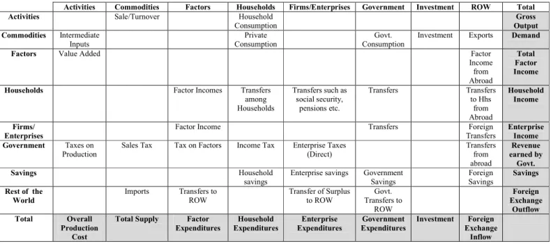
Social Accounting Matrix
The main database for building CGE models is a Social Accounting Matrix (SAM). Unlike a square I-O matrix, this is a rectangular system. There naturally arises a need to extend the I-O system to capture the flows in a specific commodity by industry format. The reason for this is that firms usually produce several commodities or provide diversified set of services. And grouping these commodities into industries can be intricate and sometimes virtually impossible.
Table 3.1: Social Accounting Matrix_ an outline
Starting with the supply side, the information regarding Activities and Commodities is usually compiled with the help of Input-Output tables, which show the typical inter-industry flows. Having input-output tables in a fairly disaggregated form helps in dealing with overlapping industrial classifications. It is beneficial to have a recent set of input-output tables closer to the reference year set for SAM. In fact Social Accounting Matrices by usual convention are also regarded as an extension of input-output (IO) matrices. This is because IO matrices show the make process as well as the use process of goods in an explicit manner, due to which IO table are also known as supply and use tables. The data on the factors of production, the receipts accruing and their expenditure outlay is available through wages and profits as indicated by labor force survey and reports on national business profiles that show clearly the enterprise income and corporate profits. Similarly the information on government expenditures and receipts can be obtained from the periodically published documents on the state of the public finance. However while compiling information on government accounts caution has to be observed while putting together data on sectoral transfers and
Activities Commodities Factors Households Firms/Enterprises Government Investment ROW Total
Activities Sale/Turnover Household
Consumption Gross Output Commodities Intermediate Inputs Private Consumption Govt. Consumption
Investment Exports Demand
Factors Value Added Factor
Income from Abroad Total Factor Income
Households Factor Incomes Transfers
among Households Transfers such as social security, pensions etc. Transfers Transfers to Hhs from Abroad Household Income Firms/ Enterprises
Factor Income Transfers Foreign
Transfers
Enterprise Income Government Taxes on
Production
Sales Tax Tax on Factors Income Tax Enterprise Taxes (Direct) Transfers from abroad Revenue earned by Govt. Savings Household savings
Enterprise savings Government Savings Foreign Savings Savings Rest of the World Imports Transfers to ROW Transfer of Surplus to ROW Govt. Transfers to ROW Foreign Exchange Outflow Total Overall Production Cost
Total Supply Factor Expenditures Household Expenditures Enterprise Expenditures Government Expenditures Investment Foreign Exchange Inflow
subsidies. Similarly as many countries have embarked upon fiscal decentralization, hence the collection level of direct taxes and the incidence of public spending require equal importance. The accounts must show clearly which segment of household bears the particular tax type.
Household’s receipts and expenditures can be obtained from household integrated surveys. These surveys typically classify households according to their consumption groups. It is worth noting that labor also forms the part of factors of production, thus when recording the factors income (wages) one may choose between the household survey data, IO tables and the labor force survey statistics. The choice will depend upon; the reliability of data, the relative coincidence of reference year (with SAM) and the coverage of labor force segments.
Traditionally the figures related to savings and investment are taken from the national accounts however to capture the intricate complexities of an open economy it would be pertinent to compare e.g. the investment figures as recorded in national income accounts and the balance of payment statistics11. Foreign Direct Investment, for example will have to be taken from the latter. Similarly the information on foreign savings will come from the current account.
The overall picture however becomes a little difficult when the trade patterns under consideration are not national but regional. Usually interregional trade accounts for many countries until today are not found in a manner which is detailed enough to make use of it for policy and predictive purposes. For building a region-specific SAM one may require additional information on regional factor payments, household incomes, government receipts and expenditures, transfer payments and institutional accounts. Several countries have now embarked upon collecting and compiling this area specific information. For the case of United States for example Minnesota IMPLAN Group (MIG) has developed relational datasets from secondary data available at the national, state and county level12.
Bussolo et al. (2003) give a detailed overview of constructing multiregional SAM for use in regional environmental general equilibrium model for India. The methodology used is of particular interest as authors have provided details on several compromises at hand when confronted with regional analysis under extreme data limitations and lapses. The main national SAM for India is used as a benchmark for a start. The Annual Survey of Industries is used then to provide regional production figures. The states have been aggregated into four broad regions. The data on labour and capital
11
Balance of Payments Statistics are published by the IMF on a monthly, bi-annual and annual basis. Usually for the construction of SAM the data is derived from the BOP Yearbook.
12
stock in the manufacturing sector is again derived from the annual survey, however for primary and services sectors assumption is made that puts shares of labour and capital value added at the regional level equal to the national level. The final demand consisting of private consumption, government expenditures, investment, stock changes and exports are derived for the households from the Household Expenditure Survey. A three step procedure is followed where they first match the 819 items in the survey with the 35 sectors in SAM. Second the sectoral shares are then multiplied by the aggregated regional consumption figures and finally these consumption values are adjusted to make certain that for a given product the sum over all regions and households equal the commodity totals as shown in the national SAM. Government expenditures at the regional level are not available, therefore for estimating the consumption by regional governments, assumption is made where sectoral public expenditure composition and the total value of public expenditures as a share of GDP are kept constant for all regions13. Similar treatment is kept for the gross fixed capital formation, whose regional details are also rarely present particularly in the developing countries. For domestic (interregional) trade the export ratios across regions do not differ. Net trade flows are estimated as a residual from regional supply minus regional demand.
Categorizing Multiregional CGE Models
Regional general equilibrium models are different from the CGE models developed at the national levels in several accounts. As Vargas et al. (1999) explain that regions are relatively more open economies compared to nations. Regional openness for example in a single country requires that greater importance be attributed to trade and resource migration. This leads us to another important distinction. National CGE models require savings to be equal to investment, however the regional models allow excess savings to flow out of the region. This reason behind this is simple; entrepreneurs would not invest in region X if region Y offered higher returns.
Three different approaches are available for construction of regional CGE models: i) top-down ii) bottom-up iii) combining top-down and bottom-up to make a hybrid framework. In the top-bottom methodology, national CGE models are constructed at first to obtain the structural variables such as employment, income and output. In the second step the demands are then disaggregated into the number of regions/provinces under consideration. This implies that we can account for the regional quantities but not prices. This also means that we don’t have region-specific supply module. However as we are making use of input-output coefficients in the second step therefore local multipliers are made available which can be used for calculating the regional output, employment
13
and income effects. Once we have obtained these we can then also calculate the feedback effects. These models can easily be transformed into a dynamic system for obtaining the annual forecasts/projections. But again as explained above region-specific demand side shocks can be modeled and captured whereas the region-specific supply side shocks cannot be accounted for in the same system. We also do not take into purview the regional/provincial government balances or accounts that show the regional budgetary receipts and expenditures.
With the bottom-up method, we first have to make region-specific CGE models that provide clear details on regional variables including the information on trade and factor inflows and outflows. In the second step we link or merge these region-specific CGE models to form a single consolidated framework in which all regions bring their output produced for trade and the factors are mobile to move from one region to another. Due to the computational constraints there is of course a limit to the number of regions that can be linked without compromising the model assumptions and theoretical underpinnings. However if a bottom-up regional CGE model is designed to capture all regions in the country, then it is worthwhile to carry out a consistency check by comparing the aggregated results with a broader national level CGE with no regional disaggregation14. Over here of course the comparable variables again would be the output, employment and incomes. Despite of all the difficulties involved in building these models, they are an important tool to capture region-specific prices and quantities supplied simultaneously, which was not possible with the top-down approach. As these models start with the regional modules first, therefore we can bring in the budgetary accounts of regional governments as well. This can actually be helpful in tracing out the tax and transfer related government flows in a completely decentralized system. In usual practice, researchers make use of bottom-up method for capturing the region-specific supply side shocks15.
The hybrid (top-down and bottom-up) approach is usually used to disaggregate our framework beyond the broader regions i.e. hybrid models capture details of sub-regions/sub-provinces. In the first step, making use of a bottom-up CGE model we obtain our usual results explained above and in the second step a top-bottom approach is used to split the regional results into sub-regional details. As these steps indicate hybrid models are computationally more intricate then the bottom-up models and pose serious consistency problems depending upon the quality of sub-regional input-output database quality. For most occasions formalized I-O tables are not available for sub-regions and one has to make use of only trifle details such as sub-regional factor employment and produced outputs.
14
Top-bottom models use a dataset where national SAM is regionally disaggregated for households, production and factor markets. On the contrary bottom-up models use region-specific SAMs. See Coady and Lee Harris (2001).
15
Even the household incomes have to be captured through some form of assumptions derived from household income and expenditure surveys.
Siksamat (2000) explains the determinants of increased capital inflow in Thailand by making use of a top-down multiregional CGE model. At the top level there is a standard national CGE model based on the ORANI-F framework16. The regional component is based on the regional disaggregation as in ORANI17. As explained above the shocks are introduced at the national tier and their effects are then allocated to the seven regions, with the help of region-specific equations. At this stage it would be important to discuss further as to how the two tiers are linked. The author explains that the theoretical structure of the regional part is based on the input-output model of Leontief et al. (1965). This model works with the assumption that all regions have fixed direct input/technology coefficients and the industry’s techonology is assumed to be identical to that in the national CGE model. There are constant trade coefficients and uniform industrial shares. There national and local commodities are distinguished and local commodities are not regionally traded. The main data requirement is the regional shares of the production of national commodities. Now the allocation of economy-wide (national CGE) results to different regions involves two further changes: i) allocation of outputs from national and local industries to each region, ii) allocation of final demands to each region.
The allocation of outputs from national level to regions requires first the distribution of activity level in national industries in a manner in which the output growth of a national industry in any of the regions in the economy is equal to the output growth of that industry as projected by the national model. Second, the supply of a local commodity supplied by a specific region must equal the demand for that commodity in that region.
The regional allocation of final demands requires first the apportionment of investment. Investment in national and local industries is allocated to the regions in the exact proportion as the production. Second the household consumption at region Z for example, is attributed to the national consumption of a specific commodity under consideration and the growth of regional income relative to the growth of the national income. Third the share of demand of an imported or domestic commodity by the Government sector in region Z, remains constant. Fourth the share of region Z in the international export of a commodity remains constant. Finally to keep the growth of regional output of local industries equal to the regional output of local commodities, the assumption is
16
See Horridge et al., (1993) for details.
17
introduced where all local industries are single product industries and each local commodity is produced by only one local industry.
This top-down model is latter converted into a hybrid form where to study the surge in capital inflows another industry named infrastructure is added only for Bangkok, considering that infrastructure makes the most difference for this city which has grown at an extremely fast pace during the past few years. The main database is the national I-O data and the gross regional product for the seven regions. Usually in a top-down model for the regional component one requires regional output shares of national commodities, which of course can be derived from accounts giving details on Gross Regional Product.
Adams (2005) using a bottom-up MMRF-Green model updates the projections for greenhouse gas emissions from stationary energy source for the case of Australia. The model captures six states and two territories such that each region has its own economy as indicated by the usual practice in bottom-up regional modelling. This model is presently one of the most detailed regional models with 49 industries, 54 products, 8 states/territories and 56 sub-state regions. For a specific year the model output is obtained from the regions and then linked together for obtaining the same opening stock levels as the closing stock levels in the last period (as the model is being used for forcasting purpose). The basic framework is based on the Monash Multiregional (MMR) framework18. As in the earlier model the number of industries is limited attributable to the computational difficulties. The main agents in the model are capital creators, industries, households, governments and foreigners. The capital creators produce sector-specific capital and the sectors produced a single commodity. Apart from the regional government in the model there is only one household in each region. Federal government has been explicitly included. Behaviour of foreigners is captured through separate treatments for export demand and import supply product curves. As in usual CGE modelling practice the regional demand and supply of commodities is determined through optimizing behaviour of agents in a competitive setting. Factors such as capital and labour are mobile and can change a region which implies that the regional employment and relative rates of returns are reflected by each region’s stock of productive resources. Industry’s demand for factors of production is again determined through optimization. Market clearing process allows the demand and supply behaviour to interact. However there are two separate blocks for regional labour markets and the other for regional and federal government balances.
18
The database requirement of MMR considerably differs from the top-down model discussed earlier. This model makes use of multiregional I-O table, regional demographic/employment information, regional and federal government budgetary details. However as explained by the author, the Australian Bureau of Statistics (ABS) does not compile multiregional input-output tables, therefore the national I-O table is disaggregated by first splitting the columns using industry and final demand regional proportions. Second the rows are split using interregional trade data. Finally the re-balancing procedures are employed for making sure that the output and sales of regional sectors equal in multiregional input-output table. Another issue is the non-availability of reliable estimates of substitution elasticities between domestic products from different regions. Therefore these values have been assumed keeping in consideration that different domestic varieties of a good are relatively close substitutes than are domestic or imported varieties. Other assumptions include those that are required for making MMR dynamic.
Spatial Networks and CGE Models
Recently the realization that CGE models lack consistency with spatial networking, regional location theories and the local level economic development policies has widely grown. Partridge and Rickman (2004) argue that regional CGE modelers have not been able to successfully change the conceptual background and parameterization from the international/national level to the regional level. Such model structures which base themselves upon the traditional national level settings fail to capture the region level dynamics. The excessive reliance on the international trade elasticities by the current CGE models provides an inaccurate responsiveness of regional settings to policy changes. Secondly the factors determining the responsiveness in the international trade literature greatly differ from the regional location theory which suggests that responses are determined by spatial proximity of customers and other firms19. Apart from the regional location perspective, CGE models can also gain from the micro-regional equilibrium approach in quality of life literature20. In this case one equalizes the household utility and firm profits across the regions under consideration and it is the relative attractiveness of a region to the potential firms and households that determines the eco-geographic distribution of activities. Another stream of literature that requires attention by the CGE modelers is the regional economic development studies. These studies largely focus on the regional living standards, availability of amenities and migration patterns21.
19
See Patridge and Rickman (1998).
20
See Roback (1982), Blomquist, Berger and Hoehn (1988), Beeson and Eberts (1989) for details.
21
Authors mainly point five critical issues that need to be addressed in the prevalent regional modelling specification. First the researchers must develop new basis to recognize that interactions between nations are substantially different from the interactions that take place in the proximity of a region. Second the outcomes of economic development at local level must be incorporated in the labor market specifications. There is a growing need for regional specification that allows incomplete migration and permanent employment rate changes. Third the models must indicate the time frame for policy changes. Models providing attractive results without specific timeframe certainly do not satisfy those who are on the implementation end. Therefore it is important that regional CGE frameworks are able to forecast the time path of responses to policy alterations22. Fourth the major factor that contributes to the transmission of growth benefits for local residents is the inter-commuting, and for smaller areas the models should be able to incorporate these area-specific linkages. Finally the demonstration of the model should be in a manner which is consistent with the broad theory, reflects the dynamic behaviour and can be validated in the light of other empirical evidence.
Emphasizing the above perpective Lofgren and Robinson (1999) develop a spatial-network, mixed complimentary CGE model which augments the general equilibrium settings and partial equilibrium programming model. For the purpose of their case study the structure of the model is engineered to capture a developing African country such as Mozambique with only one major port city that links the countrys produced goods and services to the rest of the world. The dataset used is a multi-region SAM which suggests that authors are following the bottom-up approach23. The module-wise specifications are such that the country is divided into regions in a manner that two small (rural) regions interact with the urban region (port city) and this urban city then bridges the rural with boarder region (which represents the link with rest of the world). There is no direct trade between the two rural regions or between any rural region and the border region. It is the urban region that will provide part of its rural purchases of the non-food crop to the border region for export to the rest of the world. Similarly the urban region purchases high-value crops in the form of imports coming from the border region. The commodity and factor prices are being determined through perfectly competitive regional markets.
22
This problem is to some extent solved through dynamic regional CGE models which are not commonly found in the literature. See FEDERAL-F dynamic multiregional model of Tasmania and the rest of Australia (Giesecke 2002; 2003; Giesecke and Maddlen, 2003a; 2003b).
23
Multi-region SAMs are different from national SAMs disaggregated for production and factor markets. Multi-region SAMs are infact matrices for individual regions put together.
Interregional and external trade determines the demand for transportation services which are specified with fixed-coefficient formulation. Commodities are not differentiated according to their region of production or consumption thus representing the notion of perfect substitution. As this is a developing country’s study therefore the price taker assumption is present. Given the fundamentals of microeconomic theory the patterns of interregional trade and costs of transportation are reflected in the price gaps between commodities in different regions. There are flexible regional prices that ensure the equality between regionally supplied output and the region-specific demand. The factor market permits two regimes namely; full employment with a flexible market clearing factor price, or unemployment with a minimum factor price. Labour is permitted to be mobile between sectors but not regions and agricultural land and capital are only mobile with in the agriculture sector. With the help of different simulations like the impact of higher world prices or reduced domestic transportation costs, authors show that this CGE model framework that incorporates a multi-region spatial network along with region-specific transportation costs is superior to the traditional setting where models of a single region are simulated with the national economy as given and no provision for interregional and nation-region feedbacks.
4. LINKED REGIONAL MODELS
In this section we discuss a different approach that tries to link two different types of models. Researchers have combined econometric models with I-O models to gain some additional space for analyzing the regional impacts. Usually the econometric structure at top is supposed to render the broad area-specific results which are then disaggregated at the area-specific industry or farm level.
Econometric Modelling for Regional Analysis
Regional econometric models have been in use for the past 3 decades. Adams et al. (1975) explain that the basic approach is the same as in the typical Keynesian model structure, and the working resembles the small country scenario, where the external environment is taken as given. Similarly in regional modelling the national economy and its changes are taken as given, the only causation is from national to region but not vice versa. This also implies that regional econometric models are built as a satellite of the national economy. Therefore in typical cases the final demand identity in the Keynesian framework can be replaced with the basic account identity for the region. As discussed in the CGE modelling case, accounts related to Gross State Product are the main database and a starting point for most econometric models as well. Problems arise on the expenditure front, where precise data requirement may not be available in a time-series. Similarly difficulties may be confronted in getting the accurate figures for non-manufacturing investment in the region. Figures
related to regional exports (and imports) may also not be available for a sufficient time period. Therefore the model can have a separate production equation for industries serving outside the regional market. For the consumption as well the authors explain that the lack of accurate data may be excused if one links output of sectors meeting local consumption to local disposable income.
In this model developed for Mississippi five different blocks are allowed to interact namely; output, employment, wage determination, personal income and tax blocks. As in typical econometric models the output block of this framework is purely demand determined i.e. the output of a given sector will respond to the demand for produced goods in that specific sector. As it is intricate to acquire data on goods absorbed locally and exported, therefore the same distinction that is allowed in economic base models is allowed here i.e. distinguishing between sectors producing for inside and outside the region. For most industries the link between local industries and national industries has to be maintained, because expansion of any industry at regional level relies heavily on the expansion of that industry at the national level. Authors explain that apart from the aforementioned, competitiveness at the national level has also to be accounted for in the model and primarily the market share of a sector carrying out production in Mississippi depends on the relative cost.
In the employment block, for each sector one labour demand equation is estimated. The basic labour demand function is derived from the CES production function where a Koyck lag is used to allow for the lagged response and other variables include technological change and wage to price ratio. Three different wage rates are estimated for manufacturing, non-manufacturing and agriculture sectors. Only the manufacturing sector wage rate corresponds to the national wage level in this sector the other two are locally determined and are also related to the wage levels in the manufacturing sector. An effective tax rate is calculated for obtaining the state level income tax collections. The effective tax is computed primarily in terms of the on-going fiscal year’s receipts and past year’s tax base and rate.
However the regional econometric modelling with all possible details ignores the supply side constraints on the regional economic growth. This mainly justifies the reason for the popularity of CGE models. Foreman-Peck and Lungu (2000) emphasize that purely demand side forecast derived from the Keynesian or I-O models permit over-optimism about the effectiveness of active policy programs, whereas CGE models capture both supply and demand sides along with the information on time adjustment paths of variables.
To partially overcome the above mentioned issue, researchers have recently started linking I-O models with econometric models. Despite of both being demand driven, I-O model can provide supply adjustments as a result of demand shocks, therefore representing a general equilibrium state. On the other hand econometric models typically represent economies in a partial-equilibrium or disequibliurm states. Some of the differences in both modelling frameworks in fact provide the main motivation of linking the two together. Econometric models for example are dynamic, responsive to price changes, can be used as a forecasting tool and can provide inferential results. I-O models on the contrary are not dynamic, not responsive to price fluctuations and may not be a good forecasting tool, however they provide a greater level of disaggregation and therefore better picture for impact analysis particularly in a multiregional model.
Rey (1999) explains the various channels through which I-O models can be linked to econometric models. As gross regional product is the sum of consumption, investment, government outlays and net exports, therefore traditionally it is the personal consumption that is regarded as a more plausible bridge for linking. However most regional models are not trying to endogenize investment, exports and government expenditures, which is not the case in simple I-O models where all the demand components are regarded as exogenous. Isolated I-O models also carry the restrictive assumption of a fixed employment-output ratio. This can be relaxed by introducing labour demand function in the econometric model. The author also explains how sensitive the results could be depending upon the linkage methodology. Care must be considered while linking, running and interpreting the integrated frameworks. This is primarily because econometric models can account for uncertain behaviours whereas I-O models are purely deterministic. Thus combining the two raises some inferential issues. Secondly for multiregional cases, both I-O and econometric models can be used for representing the linkages, however when we work with the integrated set-up then both models cannot not be extended for establishing multiregional links. We will have to make a choice regarding the best possible mode for multiregional/interregional relationships.
Rey (1998) explains the three classes of integrating strategies namely: linking, embedding and coupling. The linking procedure can be undertaken into two directions. First, from I-O to econometric model where demand shock is indicated by the researcher and output from the I-O module is used to derive the econometric equations such as for labor demand. Second, from Econometric to I-O model where the shock is undertaken in the former module i.e. the change in final demand is endogenous. In the embedding technique the output from the I-O model is inserted in econometric equations. This insertion can take two forms; incorporating the I-O results in a
structural econometric setting or in a time-series setting. Finally the coupling method is an extension of the linking approach wherein we integrate I-O and econometric models in a manner that represents a fully simultaneous framework. This implies that we can now have a responsive feedback mechanism at hand. However coupling method is the most data intensive out of the three mentioned. Yen (1998) describes a regional model for Portland-Vancouver where embedded I-O coefficients are being used as explanatory variables in the employment sector equations. Primarily the model has been used for forecasting population and employment growth. The model combines I-O table with econometric module using an inter-industry demand variable (IDV) for industrial employment equations24. Regional wage rates, personal income and regional production are econometrically estimated. However contrary to most embedding procedures the parameter associated with IDV is determined through regression and not pre-determined.
5. REGIONAL ECONOMIC MODELLING IN IRELAND
Before exploring the prospects of regional economic model for Ireland, it would be relevant to discuss about some of the present economy-wide models that have been in use or are being presently employed for policy analysis and evaluation. Henry (1986) provides a comprehensive history of economic modelling in Ireland. The first documented model was the Geary Decision Model, which was an I-O model designed for the medium term economic projections in a 9-sector framework. The model was published in 1964 and provided simulation solution until 1970. Second was the Simpson Medium Term Planning Model for Ireland published in 1968. The I-O sectors were extended to 16 and linear programming methodology was used to maximize household consumption. The main constraints on the objective function included labour, capital, balance of payments and the I-O interrelations. The author presents multisectoral model of the Irish economy based on the Scottish Medium Term Simulation Model (McGilvray 1981). Fundamental motivation behind this model for Irish economy was to offer a plausible framework for making employment projections for a period between 1987 to 1992. All macro variables are patternised to fit the 17 sector Social Accounting Matrix. The traditional I-O analysis of final demand is carried out for acquiring the initial information. The main dataset used was the 1972, 85 sector I-O table. Bradley and Fanning (1984) also discuss a macrosectoral model for income distribution analysis in Ireland, however the analysis is aggregate and agriculture, manufacturing and services sectors are analysed. This model does provide a prototype of analysis in a less technical manner, relying purely on national accounts data.
24
Amongst the recent examples O’Toole and Matthews (2002) use a CGE model for agriculture sector analysis. Based on the perfect competition assumptions, this is a standard static model which does not allow capital accumulation. However the model allows for multiplicity of household categories, export destinations, land and labour types. The core database is the social accounting matrix derived from the 1993 I-O tables25. However the table has been further disaggregated for sectors like agriculture, forestry and fishing. The 1994-95 Household Budget Survey has been used to extend the I-O table into a Social Accounting Matrix. There is a reconciliation process through which two different aggregations of I-O table are linked. The first is the 41 by 41 I-O tables from CSO for 1993. This dataset provides collective domestic and imported flows at basic and producer prices26. The second data base documented in O’ Connor and Matthews (2000) provides 33 by 33 domestic IO table at basic prices giving disaggregated information on agriculture, forestry and fishing sectors. The import matrix at basic prices is calculated by subtracting the latter table from the former and a separate matrix is estimated for imports of farm level produce.
An additional sector dwellings is added due to the number of backward and forward linkages associated with this sector and due to the fact that house prices have played a major role in the overall Irish economy during the past few years. As in usual practice labour costs have been included at gross level, however as there is little information as to how the wage rates should be calculated therefore constant wage differentials are picked from the Household Budget Survey. The mapping of the wages received by occupational groups with household groups is carried out. By taking representative geographical areas urban and rural household incomes are divided into different occupational groups as exact figures for rural and urban regions are not available. As authors explain that this approach also helps in capturing the importance of off-farm employment at the household level.
The taxation treatment has been carried with the help of a microsimulation module wherein marginal tax rate for each tax unit is determined and reweighed27. The overall household expenditure is sub-divided into the three household types: urban, farm and other rural. Marginal household budget shares are calculated for each commodity and to calibrate the linear expenditure system three separate calculations are done for; a) average budget share of each good per household b) Frisch parameter c) expenditure elasticities of each household type for each good. There is special treatment for capturing the effects of direct subsidies and indirect subsidies. Ireland being a net
25
For details on database see O’Toole and Matthews (2001)
26
For details see CSO (1999)
27
exporter of agriculture, the import duties are ignored. Armington elasticities are taken from Dimaranan, McDougall and Hertel (1998). The model covers 34 industries including 7 farm oriented production categories. As the main focus of this framework is to evaluate the impacts of Common Agriculture Policy therefore the distinction between different land types and labour categories plays an important role28.
Another model used for agriculture sector analysis is presented by Binfield, Donnellan and McQuinn (2000). The model is the result of collaboration between Irish Government and Food and Agricultural Policy Research Institute (FAPRI)29. The model tries to focus on the links between beef and input sectors. It would be important to discuss something about the foundations of FAPRI model that has been applied in other countries as well. It is a partial equilibrium model, and covers the global multi commodity trading patterns, which is to say that macroeconomic factors such as economic growth rate, Producer price indices, interest rate and exchange rate in the economy are exogenous.
The framework is fairly detailed at the local, national and international level, however as the authors point out that this system maybe of immense benefit to people dealing with output and pricing in the agriculture sector and not of as much importance to people dealing with purely financial aspects (like taxation issues) of domestic and international trade in agriculture. In comparison to the earlier efforts of modelling agricultural production in Ireland, the FAPRI model provides a relatively greater flexibility. Fundamentally the model is econometric that offers a decade long projections for the agriculture production. These projections take account of the Agenda 2000 reforms and a sensitivity analysis is carried out with varying exchange rates. As regards the international linkage, the Irish module is not directly linked with the World model, however there is an indirect linkage through the EU module. The small country and price taker assumption is embedded in the framework.
There are no feedback changes as regards the link between the agriculture sector and the rest of the economy. However within the agriculture sector there is fair enough scope of analyzing the causal effects. The intermission effects between the responses of a demand increase in beef sector for example and the consequent rise in the demand for inputs utilized by beef sector and the resultant decreases in the resources vested with other sectors have been modeled in detail. For major commodity groups individual production functions have been estimated using a modular approach.
28
Latter the model has been used for applications in other sectors as well.
29
The costs of production are part of the input block and particular focus is giving to the costs of feed for the producers of livestock. As we have the price taker assumption working in the background therefore it would be of relevance to note that these costs of feed or the price of beef is the one that is determined at the EU tier and then taken as exogenous in the model. There can be other application of this FAPRI-Ireland model, however the beef – input application was taken up due to the fact that beef output is the most significant component in Irish agriculture.
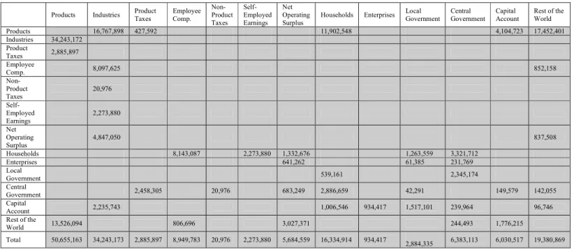
Perhaps of greatest relevance to our topic is the recent collaborative project by Border, Midland and Western (BMW) Regional Assembly in Ireland. The project has resulted in the completion of a SAM based model for the BMW region in Ireland. The main database used has been the one given by CSO that contains 36 product sectors and the main balances related to the factors of production, rest of the world and the institutions. SAM based multiplier analysis has been carried out to help the policy makers in improving their understanding of backward and forward linkages. A policy application using this model tries to capture the impact of Western Rail Corridor Scenario, as recently there has been growing interest in reestablishing the North-South rail linkage30.
To discuss the main findings of this report, we can first look at the following aggregate SAM for the BMW region that presents the broader picture on the linkages between various sectors.
Table 5.1: Aggregate BMW SAM, 2000 (thousands euros)
30
From Sligo to Limerick
Products Industries Product Taxes Employee Comp. Non-Product Taxes Self-Employed Earnings Net Operating Surplus
Households Enterprises Local Government Central Government Capital Account Rest of the World Products 16,767,898 427,592 11,902,548 4,104,723 17,452,401 Industries 34,243,172 Product Taxes 2,885,897 Employee Comp. 8,097,625 852,158 Non-Product Taxes 20,976 Self-Employed Earnings 2,273,880 Net Operating Surplus 4,847,050 837,508 Households 8,143,087 2,273,880 1,332,676 1,263,559 3,321,712 Enterprises 641,262 61,385 231,769 Local Government 539,161 2,345,174 Central Government 2,458,305 20,976 683,249 2,886,659 42,291 149,579 142,055 Capital Account 2,235,743 1,006,546 934,417 1,517,101 239,964 96,746 Rest of the World 13,526,094 806,696 3,027,371 244,493 1,776,215 Total 50,655,163 34,243,173 2,885,897 8,949,783 20,976 2,273,880 5,684,559 16,334,914 934,417 2,884,335 6,383,113 6,030,517 19,380,869
The main findings indicate that in the year 2000, the total worth of products produced in the BMW region was 36 billion euros. About 46 percent of gross value added was paid to employees in the form of salaries and 2.3 billion euros were given to self-employed. 4.8 billion euros was the net operating surplus generated and 62 percent of this surplus was paid to investors outside the region. The sectors corresponding to the high multipliers included office machinery, computer services, wood products and agriculture sector.
The basic working of the model is such that at the first stage a specific policy scenario or shock is constructed that for example changes the demand for specific sectors in the economy. Once the quantum of change is decided, it is then introduced in the SAM multiplier matrix. This matrix then provides us with region-specific sector-wise change in output, income and value added.
6. RESEARCH AGENDA
Given the recent growth experienced by the Irish economy and the upbeat forecast presented by the ESRI in their medium term framework, one can expect more intricate and complex economic linkages in future. Economic expansion leads to strengthening of inter-linkages and interdependencies between the productive sectors in the economy. It is not only the multiplier effects that become important, in fact the lag period become shorter the more the economy is mobilized. This is particularly true if the analysis pertains to the regional sphere. Under such a milieu it becomes increasingly important to have a tool that can help the policy makers to evaluate the effects of changes in one policy across on markets, sectors and institutions across the board. Such a task can certainly not be accomplished by the traditional partial equilibrium or disequilibrium models.
One may however look towards the multiregional CGE models that can assist in the evaluation and assessments related to regional production and employment patters. To our knowledge, at present there is no such model of Irish economy. Hence there is a need now to discuss the kind of inputs that may be required for moving towards such a research agenda.
The scope of such a model will largely depend upon the number of regions selected and the quality of data available. However for the time being one can assume that our regional disaggregation will be at county level. The key output of our model will include that region’s commodity wise
production, employment, income and institutional balances. The key input of course would be the regional database of CSO and the SAM built by the BMW regional assembly.
For the hybrid models one may require additional data information such as; region wise industry types and farm types (and their input requirements), region wise output specification (how does the livestock production in Donegal differ from Galway), types of crops produced, issues regarding land quality, seasonal specialization and variation in output, regional labor statistics, regional quantity and quality of capital stock, regional technology costs, regional domestic consumption and export31.
Apart from the national I-O table published by the CSO following datasets would be additionally required in order to construct a top-down model or to build a multiregional SAM for bottom-up CGE model.
Table 6.1: Data Requirements for Multiregional CGE Model
Top-down Bottom-up
Gross Regional Product Accounts32 Gross Regional Product Accounts33 Census of Agriculture Census of Agriculture
Manufacturing Inputs and Commodities Survey Manufacturing Inputs and Commodities Survey Census of Industrial Production Census of Industrial Production
Industrial Employment and Earnings Industrial Employment and Earnings Household Income and Expenditure Survey Household Income and Expenditure Survey
National Income and Expenditure Regional Accounts from Agriculture and Manufacturing Regional Population Statistics Census of Building and Construction
Annual Services Inquiry34
Product Sales Statistics (PRODCOM) Quarterly National Household Survey Census of Population
Regional Governmental Accounts Data on local taxes and transfers National Income & Expenditure
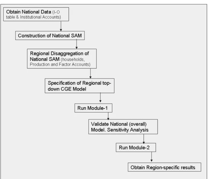
Deriving lessons from the Australian experiences, one realises that it is advisable to take a start from the top-down CGE model, where national CGE models are constructed at first to obtain the structural variables such as employment, income and output. In the second step the demands are then disaggregated into the number of regions/provinces under consideration. This implies that we can account for the regional quantities but not prices. This also means that we don’t have region-specific supply module. However as there we are making use of input-output coefficients in the
31
Technology costs may also indicate the regional cropping costs in case of for example expansion in extension services.
32
Including County incomes.
33
Including County incomes.
34