Are Stationary Hyperinflation Paths Learnable?

No. 2004/15

Are Stationary Hyperinflation Paths

Learnable?

Center for Financial Studies

The Center for Financial Studies is a nonprofit research organization, supported by an association of more than 120 banks, insurance companies, industrial corporations and public institutions. Established in 1968 and closely affiliated with the University of Frankfurt, it provides a strong link between the financial community and academia. The CFS Working Paper Series presents the result of scientific research on selected top-ics in the field of money, banking and finance. The authors were either participants in the Center´s Research Fellow Program or members of one of the Center´s Research Pro-jects.

If you would like to know more about the Center for Financial Studies, please let us know of your interest.

* _{Financial support from US National Science Foundation, the Academy of Finland, Yrjö Jahnsson Foundation,}

Bank of Finland and Nokia Group is also gratefully acknowledged.

1 _{Klaus Adam, CEPR, London, University of Frankfurt, Mertonstr.17, PF94, 60054 Frankfurt am Main, Germany} 2

CFS Working Paper No. 2004/15

Are Stationary Hyperinflation Paths Learnable?

Klaus Adam

, George W. Evans

and Seppo Honkapohja

March 17, 2003

Abstract:

Earlier studies of the seigniorage inflation model have found that the high-inflation steady state is not stable under adaptive learning. We reconsider this issue and analyze the full set of solutions for the linearized model. Our main focus is on stationary hyperinflationary paths near the high-inflation steady state. The hyperinflationary paths are stable under learning if agents can utilize contemporaneous data. However, in an economy populated by a mixture of agents, some of whom only have access to lagged data, stable inflationary paths emerge only if the proportion of agents with access to contemporaneous data is sufficiently high.

JEL Classification: C62, D83, D84, E31

1

Introduction

The monetary inflation model, in which the demand for real balances de-pends negatively on expected inflation and the government uses seigniorage to fund in part its spending on goods, has two steady states and also perfect foresight paths that converge to the high inflation steady state.1 _{The paths}

converging towards the high steady state have occasionally been used as a model of hyperinflation, see e.g. (Fischer 1984), (Bruno 1989) and (Sargent and Wallace 1987). However, this approach remains controversial for several reasons. First, the high inflation steady state has “perverse” comparative static properties since an increase in seigniorage leads to lower steady state inflation. Second, recent studies of stability under learning of the high

in-flation steady state suggest that this steady state may not be a plausible equilibrium.

(Marcet and Sargent 1989) and (Evans, Honkapohja, and Marimon 2001) have shown that the high inflation steady state is unstable for various ver-sion of least squares learning. (Adam 2003) has obtained the same result for a sticky price version of the monetary inflation model with monopolistic competition. (Arifovic 1995) has examined the model under genetic algo-rithm learning and the economy appears always to converge to the steady state with low, rather than high inflation. Experimental work by (Marimon and Sunder 1993) also comes to the conclusion that the high inflation steady state is not a plausible outcome in the monetary inflation model.

The instability result for the high inflation steady state under learning has been derived under a particular assumption about the information sets that agents are assumed to have. (Van Zandt and Lettau 2003) raise questions about the timing and information sets in the context of learning steady states. They show that, under what is often called constant gain learning, the high inflation steady state in the Cagan model can be stable under learning with specific informational assumptions.2 _{In a related but different model, (Duffy}

1994) showed the possibility of expectationally stable dynamic paths near an indeterminate steady state.

The monetary inflation model, like that of (Duffy 1994), has the im-portant feature that the temporary equilibrium inflation rate in period t

1_{The model is also called the Cagan model after (Cagan 1956) .}

2_{However, constant gain learning is most natural in nonstochastic models, since}

other-wise convergence to REE is precluded. In this paper we allow for intrinsic random shocks and thus use “decreasing gain” algorithms, consistent with least squares learning.

depends on the private agents’ one-step ahead forecasts of inflation made in two successive periods, t ₋1 and t. Except for some partial results in (Duffy 1994) and (Adam 2003), the different types of rational expectations equilibria (REE) in such “mixed dating models” have not been examined for stability under learning. In this paper we consider this issue, paying careful attention to different possible information sets that agents might have. In particular, we show that stationary AR(1) paths, as well associated sunspot equilibria around an indeterminate steady state, such as the high inflation steady state, are stable under learning when agents have access to contempo-raneous data of endogenous variables. However, this result is sensitive to the information assumption. If the economy has sufficiently many agents who base their forecasts only on lagged information, then the results are changed and the equilibria just mentioned become unstable under learning.

2

The hyperin

fl

ation model

In the standard hyperinflation model real money demand is a linearly de-creasing function of expected inflation, i.e.

md_t =ψ₀₋ψ₁E_t∗xt+1 withψ0 >ψ1 >0

wheremd

t denotes real money demand and xt+1 the inflation factor fromtto

t+ 1. Here E∗

txt+1 denotes expected inflation, which we do not restrict to

be fully rational (we will reserve Etxt+1 for rational expectations). Money

demand functions of the above form can be generated by monetary overlap-ping generations models with log-utility functions. Alternatively they can be viewed as a log-version of the (Cagan 1956) demand function.

Real money supplyms

t is given by

ms_t = mt−1 xt

+g+vt

where mt−1 denotes the real value of outstanding balances in t −1, g is

the mean value of real seigniorage, and vt is a stochastic seigniorage term

assumed to be white noise with small bounded support and zero mean.3 _This

formulation of the seigniorage equation is standard, see e.g. (Sargent and

3_{More generally the monetary shock could be allowed to be a martingale difference}

Wallace 1987) . The above equation simply states that government purchases of goods is financed by printing money, i.e. g+vt= (Mts−Mt−1)/Pt, where

Mt denotes the nominal money stock and Pt the price of goods, so that

mt=Mt/Pt and xt =Pt/Pt−1. It would also be straightforward to allow for

a fixed amount of government purchases financed by lump-sum taxes. Market clearing in all periods implies that

xt = ψ₀₋ψ₁E∗ t−1xt ψ₀₋ψ₁E∗ txt+1−g−vt . (1) Provided g < gmax=³pψ_{0 −}pψ₁´ 2

there exist two noisy steady states, with different mean inflation rates x, given by the quadratic

ψ1x2 −(ψ1+ψ0−g)x+ψ0 = 0. (2)

We denote the low inflation steady state by xl _{and the high inflation steady}

state by xh. Throughout the paper we will assume that g < gmax so that both steady states exist. As shown in Appendix A.1, the low inflation steady state is locally unique, while there is a continuum of stationary REE in a neighborhood of the high inflation steady state.

The model (1) can be linearized around either steady state, leading to a reduced form thatfits into a general mixed dating expectations model taking the form

xt =α+β1Et∗xt+1+β0Et∗−1xt+ut, (3)

whereutis a positive scalar timesvt. It is convenient to study learning within

the context of the linearized model (3), and this has the advantage that our results can also be used to discuss related models with the same linearized reduced form, e.g. the one of (Duffy 1994).

The linearization of the hyperinflation model is discussed in detail in Appendix A.1. We here note that equation (1) implies β₁ > 0 and β₀ < 0 for the linearization at either steady state. Furthermore the coefficients (α,β₀,β₁) at either steady state are functions of the parameters ω and ξ only, where

ω = ψ1

ψ₀ and ξ = g gmax.

3

The mixed dating model

We start by determining the complete set of rational expectations equilibria for model (3). These can be obtained as follows. In a rational expectations equilibrium (REE) the forecast error

η_t =xt−Et−1xt

is a martingale difference sequence (MDS), which together with (3) implies that

xt=α+β1(xt+1+ηt+1) +β0(xt+ηt) +ut.

Solving for xt+1 and lagging the equation by one period delivers

xt=−β−11α+β− 1 1 (1−β0)xt−1+ηt+β− 1 1 β0ηt−1−β− 1 1 ut−1

One can decompose the arbitrary MDSη_tinto a component that is correlated with ut and an orthogonal sunspot η

0

t:

η_t=γ₀ut+γ1η0t

The sunspot η0

t is again a MDS. Moreover, sinceηt is an arbitrary MDS, the

coefficients γ0 and γ1 are free to take on any values. This delivers the full

set of rational expectations solutions for the model: xt=− α β1 +(1−β0) β1 xt−1+γ0ut+ (β0γ0−1) β1 ut−1+γ1η0t+ β0γ1 β1 η0t−1 (4)

Since γ0 and γ1 are arbitrary there is a continuum of ARMA(1,1) sunspot

equilibria.

Forγ₀ = 1 and γ₁ = 0 we obtain the stochastic steady state solution xt=α(1−β1−β0)−1+ (1−β1 −β0)−1ut, (5)

while setting γ₀ =β−₀1 and γ₁ = 0 yields an AR(1) solution xt=−β−11α+β−

1

1 (1−β0)xt−1+β−01ut (6)

For the hyperinflation model, stability of steady state solutions (5) has been studied in (Marcet and Sargent 1989)4 and (Evans, Honkapohja, and

4_{Marcet and Sargent actually formulate the forecasting problem in terms of forecasting}

Marimon 2001). In this paper, we will examine the stability of the full set of ARMA(1,1) solutions (4) and how their stability under learning is affected by the information sets. As shown in Appendix A.1, the ARMA(1,1) solutions near the high inflation steady state are stationary because 0<β−₁1(1₋β0)<

1 for the linearization at xh.

4

Learning with full current information

We first consider the situation where agents have information about all vari-ables up to time t and wish to learn the parameters of the rational expecta-tions solution (4). As is well-known, the condiexpecta-tions for local stability under adaptive learning are given by expectational stability (E-stability) conditions. Therefore, wefirst discuss the E-stability conditions for the REE, after which we take up real time learning.

4.1

E-stability

Agents’ perceived law of motion (PLM) of the state variable xt is given by

xt=a+bxt−1+cut−1+dη0t−1+ζt (7)

where the parameters (a, b, c, d) are not known to the agent but are estimated by least-squares, and ζ_t represents unforecastable noise.

Substituting the expectations generated by the PLM (7) into the model (3) delivers the actual law of motion (ALM) for the state variable xt:

xt= (1−β1b)− 1

[α+ (β₁ +β₀)a] (8)

+ (1₋β₁b)−1£β₀bxt−1+ (1 +β1c)ut+β0cut−1+β1dη0t+β0dη0t−1

¤

in the ALM, the T-map in short, is given by a_→ α+ (β1+β0)a 1₋β₁b b_→ β0b 1₋β₁b c_→ β0c 1₋β₁b d_→ β0d 1₋β₁b

Since the variables entering the ALM also show up in the PLM, the fixed points of the T-map are rational expectations equilibria. Furthermore, as is easy to verify, all REE’s are also fixed points of the T-map.

Local stability of a REE under least squares learning of the parameters in (7) is determined by the stability of the differential equation

d(a, b, c, d)

dτ =T(a, b, c, d)−(a, b, c, d) (9) at the REE. This is known as the E-stability differential equation, and the connection to least squares learning is discussed more generally and at length in (Evans and Honkapohja 2001). If an REE is locally asymptotically stable under (9) then the REE is said to be “expectationally stable” or “E-stable.”

Equation (9) is stable if and only if the eigenvalues of

DT =       β1+β0 1−β₁b −(α+(β1+β0)a)β1 (1−β1b)2 0 0 0 β0 (1−β₁b)2 0 0 0 ₋ β1β0c (1−β1b)2 β0 1−β1b 0 0 ₋ β1β0d (1−β1b)2 0 β0 1−β1b       (10)

have real parts smaller than 1 at the REE. At the REE we have

a=₋β−₁1α (11)

b=β−₁1(1₋β0) (12)

c, d:arbitrary and the eigenvalues of DT are given by:

λ1 = 1 +

β1

β₀; λ2 = 1

The eigenvectors corresponding to the last two eigenvalues are those pointing into the direction of cand d, respectively. As one would expect, stability in the point-wise sense cannot hold for these parameters and in contexts such as these, E-stability is defined relative to the whole class of ARMA equilibria. A class of REE is said then said to be E-stable if the dynamics under (9) converge to some member of the class from all initial points sufficiently near the class. We can then summarize the preceding analysis:

Proposition 1 If β₁ > 0 and β₀ < 0 or if β₁ < 0 and β₀ > 1 the set of ARMA(1,1)-REE is E-stable.

Figure 1 illustrates these conditions in the (β₀,β₁)-space. The light grey region indicates parameter values for which the ARMA equilibria are E-stable but explosive. Ifβ1 andβ0lies in the black region, then the ARMA equilibria

are both E-stable and stochastically stationary. FIGURE 1 HERE

Since β1 > 0 and β0 < 0 for the high steady state in the hyperinflation

model, Proposition 1 implies that the set of stationary ARMA(1,1)-REE is E-stable.

We remark that Proposition 1 applies to any model with reduced form (3). In particular, in the model of (Duffy 1994) we have ₋β₁ =β₀ >1, and thus this proposition confirms his E-stability result for the stationary AR(1) solutions and, more generally, proves E-stability for stationary ARMA(1,1) sunspot solutions.

4.2

Real time learning

Next we consider real time learning of the set of ARMA equilibria (4). This section shows that stochastic approximation theory can be applied to show convergence of least squares learning when the PLM of the agents has AR(1) form and the economy can converge to the locally determinate AR(1) equilib-rium (6). For technical reasons the stochastic approximation tools cannot be applied for the continuum of ARMA(1,1)-REE. Therefore, real time learning of the class (4) REE will be considered in section 7 using simulations.

Assume first that agents have the PLM of AR(1) form, i.e.

The parameters aand bare updated using recursive least squares using data through period t, so that the forecasts are given by

E_t∗xt+1 =at+btxt,

E_t∗₋₁xt=at−1+bt−1xt−1.

Substituting these forecasts into (3) yields the ALM xt= α+β₀at−1+β1at 1₋β1bt + β0bt−1 1₋β1bt xt−1 + 1 1₋β1bt ut. (14)

Parameter updating is done using recursive least squares i.e.

µ at bt ¶ = µ at−1 bt−1 ¶ +ϑtR−t1(xt−1−at−1−bt−1xt−2) µ 1 xt−2 ¶ , (15) where Rt is the matrix of second moments, which will be explicitly specified

in the Appendix, andϑtis the gain sequence, which is a decreasing sequence

such as t−1_.5 _{In Appendix A.2 we prove the following result:}

Proposition 2 The AR(1) equilibrium of model (3) is stable under least squares learning (15) if the model parameters satisfy the E-stability conditions β1 >0 and β0 <0 or β1 <0 and β0 >1.

Since E-stability governs the stability of the AR(1) solution under least squares learning, the stationary AR(1) solutions in the hyperinflation model are learnable. The same result holds for the AR(1) solution in a stochastic version of the model of (Duffy 1994).

5

Learning without observing current states

The observability of current states, as assumed in the previous section, in-troduces a simultaneity between expectations and current outcomes. Tech-nically this is reflected in xt appearing on both sides of the equation when

substituting the PLM (7) into the model (3). To obtain the ALM one first has to solve this equation for xt. Although this is straightforward

mathe-matically, it is not clear what economic mechanism would ensure consistency

5_{See Chapter 2 of (Evans and Honkapohja 2001) for the recursive formulation of least}

between xt and the expectations based on xt. Moreover, in the non-linear

formulation there may even exist multiple mutually consistent price and price expectations pairs, as pointed out in (Adam 2003).

To study the role of the precise information assumption, we introduce a fraction of agents who cannot observe the current state xt. Such agents in

effect must learn to make forecasts that are consistent with current outcomes, which allows us to consider the robustness of the preceding results. Thus suppose that a share λ of agents has information set

H_t0 =σ(ut, ut−1, . . . ,η0t,η0t−1, . . . , xt−1, xt−2. . .)

and cannot observe the current state xt. Let the remaining agents have the

“full t”-information set

Ht =σ(ut, ut−1, . . . ,ηt0,η0t−1, . . . , xt, xt−1. . .)

Expectations based on Ht0 are denoted by Et0∗[·] and expectations based on

Ht byEt∗[·].

With the relevant economic expectations given by the average expecta-tions across agents, the economic model (3) can now be written as

xt=α+β1((1−λ)Et∗[xt+1] +λEt0∗[xt+1]) +β0 ¡ (1₋λ)E_t∗₋₁[xt] +λEt0∗−1[xt] ¢ +ut

As before, the PLM of agents with information setHt will be given by

xt=a2+b2xt−1+c2ut−1+d2η0t−1+ζt

while the PLM for agents with information set Ht0 is given by

xt =a1+b1xt−1+e1ut+c1ut−1+f1η0t+d1η0t−1+ζ

0

t.

Here ζt and ζ0t represent zero mean disturbances that are uncorrelated with

all variables in the respective information sets. Since agents with information setH_t0 do not knowxt, they mustfirst forecastxt to be able to forecastxt+1.

The forecast of xt depends on the current shocks ut and η0t, which implies

Agents’ expectations are now given by E_t∗[xt+1] =a2+b2xt+c2ut+d2η0t E_t0∗[xt+1] =a1+b1Et0∗[xt] +c1ut+d1η0t =a1+b1 £ a1+b1xt−1+e1ut+c1ut−1+f1ηt0 +d1η0t−1 ¤ +c1ut+d1η0t =a1(1 +b1) +b21xt−1+ (b1e1+c1)ut +b1c1ut−1 + (b1f1+d1)η0t+b1d1n0t−1

and the implied ALM can be written as zt=A+Bzt−1 +C µ ut η0t ¶ (16) where zt = (xt, xt−1, ut, ut−1,η0t,η0t−1) and where the expressions for A, B,

and C can be found in Appendix A.3.1.

It is important to note that the ALM is an ARMA(2,2) process and therefore of higher order than agents’ PLM. This is due to the presence of agents with H0

t information. These agents use variables dated t −2 to

forecast xt. This feature has several important implications. First, while

the T-map is given by the coefficients showing up in the ARMA(2,2)-ALM (16), calculating the fixed points of the learning process now requires us to project the ARMA(2,2)-ALM back onto the ARMA(1,1) parameter space. Second, it might appear that the resulting fixed points of the T-map would not constitute rational expectations equilibria, but rather what have been called “restricted perceptions equilibria’ (RPE). RPE have the property that agents’ forecasts are optimal within the class of PLMs considered by agents, but not within a more general class of models.6

Because our agents estimate ARMA(1,1) models, and under the current information assumptions ARMA(1,1) PLMs generate ARMA(2,2) ALMs, there is clearly the possibility that convergence will be to an RPE that is not an REE. However, as we will show below, convergence will be to an ARMA(2,2) process that can be regarded as an overparameterized ARMA(1,1) REE. Therefore, the misspecification by agents is transitional and disappears asymptotically.

The projection of the ARMA(2,2)-ALM on the ARMA(1,1)-PLM is ob-tained as follows. Under the assumption that zt is stationary equation (16)

6_{The issue of projecting a higher-order ALM back to a lower-order PLMfirst arose in}

implies

vec(var(zt)) = (I−B ⊗B)−1vec

µ Cvar µ ut η0 t ¶ C0 ¶ (17) Using the covariances in (17) one can express the least squares estimates as

T       bi ei ci fi di      =var       xt−1 ut ut−1 η0 t η0 t−1       −1 cov             xt−1 ut ut−1 η0 t η0 t−1      , xt      

The estimate for the constant

T(ai) = (1−bi)E(xt)

= (1₋bi)

A11

1_{− 1/β} 1

1−(1−λ)b2 (B11+B12)

where A11, B11, and B12 are elements of the ALM coefficients A and B, as

given in Appendix A.3.1. This completes the projection of the ARMA(2,2)-ALM onto the ARMA(1,1)-PLM.

Using Mathematica one can then show that the following parameters are

fixed points of the T-map:

(a1, b1, e1, c1, f1, d1, a2, b2, c2, d2) = (₋α/β₁,₋ρ,γ₀,γ₀ρ₋1/β₁,γ₁,γ₁ρ,₋α/β₁,₋ρ,γ₀ρ₋1/β₁,γ₁ρ) (18) where ρ= β0 β1 γ₀,γ₁ : arbitrary constants

Note that the PLMs of agents with information set Ht and Ht0 is the

same (up to the coefficients showing up in front of the additional regressors of Ht0-agents). This is not surprising since agents observe the same variables

and estimate the same PLMs.

It might appear surprising that the PLM-parameters in (18) are indepen-dent of the share λ of agents with information set Ht0. This is because one

might expect that the value ofλ would affect the importance the second lags in the ALM (18) and therefore influence the projection of the ARMA(2,2)-ALM onto the PLMs. However, it can be shown that this is not true at the

fixed point (18). Calculating the ALM implied by thefixed point (18) yields:

A(L) · 1 + (₋ 1 β₁ +ρ)L ¸ xt=A(L) · γ₀+ (₋ 1 β₁ +γ0ρ)L ¸ ut (19) +A(L) [γ₁ +γ₁ρL]η0_t+A where A(L) = −β1ρ−λ+β1ρλ β₁ρ(λ₋1)₋λ + −ρλ+β1ρ2λ β₁ρ(λ₋1)₋λL A= α((1 +ρ)λ−β1ρ(−1 +λ+ρλ)) β1(β1ρ(λ−1)−λ) .

The ARMA(2,2)-ALM (16) has a common factor in the lag polynomials. Canceling the common factor A(L) in (19) gives the ARMA(1,1)-REE (4). Fromρ= β0

β1 it can be seen that the resulting ARMA(1,1) process is precisely the ARMA(1,1) REE (4).

To summarize the preceding argument, the ALM is a genuine ARMA(2,2) process during the learning transition and this is underparameterized by the agents estimating an ARMA(1,1). However, provided learning converges, this misspecification becomes asymptotically negligible. As in the case of the ARMA(1,1)-REE, E-stability of the ARMA(1,1)fixed points are determined by the eigenvalues of the matrix

dT

d(a1, b1, e1, c1, f1, d1, a2, b2, c2, d2)

(20) evaluated at the fixed points.

As a first application of our setting, we consider the model of (Duffy 1994), which depends on a single parameter because ₋β₁ = β₀ > 1. Using Mathematica to derive analytical expressions for the eigenvalues of (20), one can show that a necessary condition for E-stability is given by

λ< (β1)

2

2 (β1) 2

−1. (21)

Thus, in this model the ARMA(1,1)-REE become unstable if a high enough share of agents does not observe current endogenous variables.

6

The hyperin

fl

ation model reconsidered

We now consider the stability of the ARMA(1,1)-REE in the hyperinflation model when a shareλof agents has informationH0

tand the remaining agents

have informationHt. Wefirst examine the case of small amounts of

seignior-age ξ_→0, for which the expressions for the linearization coefficients and the equilibrium coefficients become particularly simple. We then present some results for the general case ξ>0.

6.1

Small amounts of seigniorage

The linearization coefficients of the hyperinflation model for ξ_→0 are given by lim ξ→0α = 1 ω lim ξ→0β1 = +∞ lim ξ→0ρ= β0 β1 =₋ω

From equation (18) it then follows that in the ARMA(1,1)-REE are given by (a1, b1, e1, c1, f1, d1, a2, b2, c2, d2)

= (0,ω,γ0,−γ0ω,γ1,−γ1ω,0,ω,−γ0ω,−γ1ω).

E-stability of the ARMA(1,1)-REE is determined by the eigenvalues of the T-map. Analytical expressions for the eigenvalues are given in Appendix A.3.2. Four of these eigenvalues are equal to zero. Two eigenvalues are equal to one. The latter correspond to the eigenvectors pointing into the direction of the arbitrary constants γ₀ and γ₁. The remaining four eigenvalues si

(i= 1, . . . ,4) are functions of ω and λ, and we compute numerical stability results.

FIGURE 2 HERE

For λ values lying above the line shown in Figure 2 the ARMA(1,1) class of REE is E-unstable. A sufficient condition for instability is λ > 1/2 (since then s1 >1).

6.2

The intermediate and large de

fi

cit case

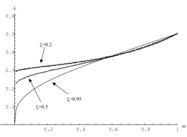
Using the analytical expressions for the eigenvalues of the matrix (20) we used numerical methods to determine critical share λ for which the ARMA(1,1)-REE becomes E-unstable for positive values of the deficit share ξ. Figure 3 displays the critical λ values for ξ values of 0.2, 0.5, and 0.95, respectively. For λ values lying above the lines shown in these figures, the ARMA(1,1) class of REE is E-unstable. For λ values below these lines the equilibria remain E-stable.

FIGURE 3 HERE

The figure suggests that λ > 0.5 continues to be a sufficient condition for E-instability of the ARMA(1,1) REE. However, critical values for λ appear generally to be smaller than 0.5, with critical values significantly lower if ω is small and ξ is high. Moreover, when ω = 0 and ξ _→ 1, these equilibria become unstable even if an arbitrarily small share of agents does not observe the current values of xt.

7

Simulations

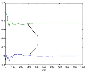
Because formal real time learning results cannot be proved for the ARMA(1,1) sunspot solutions, we here present simulations of the model under learning. These indicate that the E-stability results do indeed provide the stability conditions of this class of solutions under least-squares learning. In the il-lustrative simulations we set β1 = 2 and β0 = −0.5 and α = 0. For these

reduced form parameters the values of a and bat the ARMA(1,1) REE are a = 0 and b = 0.75. For these reduced form parameters the ARMA(1,1) REE are E-stable for λ = 0, see Figure 1, and convergent parameter paths are indeed obtained under recursive least squares learning. The parameter estimates for a typical simulation, shown in Figures 4 and 5, are converging toward equilibrium values of the set of ARMA(1,1) REE.

FIGURES 4 THROUGH 7 HERE

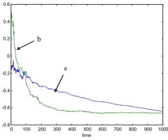
In Figures 6 and 7 the share of agents with information set Ht0 is increased

to λ = 0.5 and the ARMA(1,1) sunspot equilibria become unstable under learning. For example, at and bt are clearly diverging from the values of the

These simulation results illustrate on the one hand the possibility of least squares learning converging to stationary solutions near the high inflation steady state. On the other hand these results also show that stability de-pends sensitively on the information available to agents when their inflation forecasts are made.

8

Conclusions

In this paper we have studied the plausibility of stationary hyperinflation paths in the monetary inflation model by analyzing their stability under adaptive learning. The analysis has been conducted using a reduced form that has wider applicability. For the hyperinflation model, if agents can ob-serve current endogenous variables at the time of forecasting then stationary hyperinflation paths of the AR(1) and ARMA(1,1) form, as well as asso-ciated sunspot solutions, are stable under learning. Although this suggests that these equilibria may provide a plausible explanation of hyperinflationary episodes, the finding is not robust to changes in agents’ information set. In particular, if a significant share of agents cannot observe current endogenous variables when forming expectations, the stationary hyperinflation paths be-come unstable under learning.

A

Appendices: Technical Details

A.1

Linearization of hyperin

fl

ation model

Equation (2), which specifies the steady states, can be rewritten as x2₋ψ1 +ψ0−g

ψ1

x+ ψ0 ψ1

= 0,

from which it follows that the two solutions xl _{< x}h _{satisfy x}l_xh _{= ψ}

0/ψ1

and hence that

xl <

s

ψ0

ψ₁ < x

Linearizing (1) at a steady state xyieldsxt=α+β1Et∗xt+1+β0Et∗−1xt+ut, where β0 =− ψ1x ψ0−ψ1x and β1 = ψ1x2 ψ0−ψ1x .

Note that β₁ >0 and β₀ < 0. We remark that ₋β₀ is the elasticity of real money demand with respect to inflation and that β1 =−β0x.

For the linearized model the AR(1) or ARMA(1,1) solutions of the form (4) are stationary if and only if the autoregressive parameterβ−₁1(1₋β₀)>0 is smaller than one. Since

β−₁1(1₋β₀) = ψ0 ψ1x2

,

it follows that the solutions (4) are stationary near the high inflation steady state xh, but explosive near the low inflation steady state xl.

A.2

Proof of Proposition 2

We start by defining yt−1 = (1, xt−2)0. With this notation we write the

updating for the matrix of second moments as

Rt =Rt−1+ϑt(yt−1yt0−1−Rt−1)

and make a timing change St=Rt+1 in order to write recursive least squares

(RLS) estimation as a stochastic recursive algorithm (SRA). In terms of St

we have St=St−1+ϑt µ ϑt+1 ϑt ¶ (yty0t−St−1) (22) and St−1 =St−2+ϑt(yt−1yt0−1−St−2) (23)

for the periods t and t ₋ 1. For updating of the estimates of the PLM parameters we have (15), which is rewritten in terms of St−1 as

µ at bt ¶ = µ at−1 bt−1 ¶ +ϑtSt−−11(xt−1−at−1−bt−1xt−2) µ 1 xt−2 ¶ (24)

and µ at−1 bt−1 ¶ = µ at−2 bt−2 ¶ +ϑt µ ϑt−1 ϑt ¶ S_t−₋1₂(xt−2−at−2−bt−2xt−3) µ 1 xt−3 ¶ . (25) To write the entire system as a SRA we next defineκt= (at, bt, at−1, bt−1)0

and φ_t=   vecSκt t vecSt−1   and Xt=     xt−1 xt−2 xt−3 1    .

With this notation the equations for parameter updating are in the standard form

φt =φt−1+ϑtQ(t,φt−1,Xt), (26)

where the function Q(t,φ_t−1,Xt) is defined by (22), (23), (24) and (25). We

also write (14) in terms of general functional notation as xt=xa(φt) +xb(φt)xt−1+xu(φt)ut.

For the state vector Xt we have

    xt−1 xt−2 xt−3 1    =     xb(φt−1) 0 0 0 1 0 0 0 0 1 0 0 0 0 0 0         xt−2 xt−3 xt−4 1     +     xa(φt−1) xu(φt−1) 0 0 0 0 1 0     µ 1 ut−1 ¶ or Xt=A(φt−1)Xt−1 +B(φt−1)υt, (27) where υt= (1, ut−1)0.

The system (26) and (27) is a standard form for SRAs. Chapters 6 and 7 of (Evans and Honkapohja 2001) discuss the techniques for analyzing the convergence of SRAs. The convergence points and the conditions for conver-gence of dynamics generated by SRAs can be analyzed in terms of an asso-ciated ordinary differential equation (ODE). The SRA dynamics converge to an equilibrium point φ∗ when φ∗ is locally asymptotically fixed point of the associated differential equation. We now derive the associated ODE for our model.

For a fixed value of φ the state dynamics are essentially driven by the equation xt−1(φ) =xa(φ) +xb(φ)xt−2+xu(φ)ut−1. Now Eytyt0 = µ 1 Ext(φ) Ext(φ) Ext(φ)2 ¶ ≡M(φ). Defining ²t−1(φ) =xt−1−a−bxt−2 we compute ²t−1(φ) = (xa(φ)−a) + (xb(φ)−b)xt−2(φ) +xu(φ)υt, so that E²t−1(φ) µ 1 xt−2(φ) ¶ =M(φ) µ xa(φ)−a xb(φ)−b ¶ . These results yield the associated ODE as

d dτ µ a b ¶ =S−1M(φ) µ xa(φ)−a xb(φ)−b ¶ dS dτ =M(φ)−S d dτ µ a1 b1 ¶ =S₁−1M(φ) µ xa(φ)−a1 xb(φ)−b1 ¶ dS1 dτ =M(φ)−S1,

where the temporary notation of variables with/without the subscript 1 refers to the t and t₋1 dating in the system (22), (23), (24) and (25).

A variant of the standard argument shows that stability of the ODE is controlled by the stability of the small ODE

d dτ     a b a1 b1    =     xa(φ)−a xb(φ)−b xa(φ)−a1 xb(φ)−b1    . (28)

Next we linearize the small ODE at the fixed point a = a1 = a∗ ≡ −β−11α,

b= b1 =b∗ ≡ β1−1(1−β0). The derivative of (28) at thefixed point can be

written as DX₋I, where DX =     β−01β1 −β− 1 0 β1 1 0 0 β−01−1 0 1 β−₀1β_{1 −}β−₀1β₁ 1 0 0 β−₀1₋1 0 1    .

The eigenvalues of DX are clearly zero and the remaining two roots are 1 +β−₀1β₁ and β−₀1. The local stability condition for the small ODE and hence the condition for local convergence the RLS learning as given in the statement of Proposition 2.

A.3

Details on the Model with a Mixture of Agents

A.3.1 The ALM when some agents do not observe current states

The coefficients in the ALM (16) are

A0 =¡ ς(α/β1+ (1 +ρ)[λ(1 +b1)a1+ (1−λ)a2]) 0 0 0 0 0 0 ¢ B =         ςB11 ςB12 ςB13 ςB14 ςB15 ςB16 ς 0 0 0 0 0 0 0 0 0 0 0 0 0 ς 0 0 0 0 0 0 0 0 0 0 0 0 0 ς 0        

C =         ς(λ(b1e1+c1) + (1−λ)c2+ 1/β1) ς(λ(b1f1+d1) + (1−λ)d2) 0 0 0 0 0 0 0 0 0 0         where ς = (1/β₁₋(1₋λ)b2)−1 and B11=λb21+ρ(1−λ)b2 B12=ρλb21 B13=λb1c1+ρ(λ(b1e1+c1) + (1−λ)c2) B14=ρλb1c1 B15=λb1d1+ρ(λ(b1f1+d1) + (1−λ)d2) B16=ρλb1d1

A.3.2 Eigenvalues in the small deficit case

For the hyperinflation model with a mixture of agents, the eigenvalues of the derivative of the T-map at the ARMA(1,1)-solution near the high-inflation steady state, for small deficit values (i.e. as ξ_→0), are given by

s1 = λ2 (1₋λ)2 s2 = (1 +ρ)(₋1 +ρλ) ρ(₋1 +λ+ρλ) s3 =− 2ρ3₍ −1 +λ)λ2+ρ5_(λ2 −2λ3) +√s 2ρ3_{(−1 +λ)}2_{(1 + (−1 +ρ}2_)λ) s4 = 2ρ3₍ −1 +λ)λ2+ρ5_(λ2 −2λ3) +√s 2ρ3_{(−1 +λ)}2_{(1 + (−1 +ρ}2_)λ) s5 =s6 = 1 s7 =s8 =s9 =s10= 0 where s=ρ6λ2(4(₋1 +λ)2+ρ4λ(₋4 + 5λ)₋4ρ2(1₋3λ+ 2λ2))

References

Adam, K.(2003): “Learning and Equilibrium Selection in a Monetary

Over-lapping Generations Model with Sticky Prices,”Review of Economic Stud-ies, forthcoming.

Arifovic, J. (1995): “Genetic Algorithms and Inflationary Economies,”

Journal of Monetary Economics, 36, 219—243.

Barnett, W., J. Geweke, and K. Shell (eds.) (1989): Economic

Complexity: Chaos, Sunspots, Bubbles, and Nonlinearity. Cambridge Uni-versity Press, Cambridge.

Bruno, M. (1989): “Econometrics and the Design of Economic Reform,”

Econometrica, 57, 275—306.

Cagan, P. (1956): “The Monetary Dynamics of Hyper-Inflation,” in

(Friedman 1956).

Duffy, J. (1994): “On Learning and the Nonuniqueness of Equilibrium

in an Overlapping Generations Model with Fiat Money,”Journal of Eco-nomic Theory, 64, 541—553.

Evans, G. W., and S. Honkapohja (2001): Learning and Expectations

in Macroeconomics. Princeton University Press, Princeton, New Jersey.

Evans, G. W., S. Honkapohja, and R. Marimon (2001):

“Conver-gence in Monetary Inflation Models with Heterogeneous Learning Rules,”

Macroeconomic Dynamics, 5, 1—31.

Fischer, S. (1984): “The Economy of Israel,” Journal of Monetary

Eco-nomics, Supplement, 20, 7—52.

Friedman, M. (ed.) (1956): Studies in the Quantity Theory of Money.

University of Chicago Press, Chicago.

Marcet, A., and T. J. Sargent (1989): “Convergence of Least Squares

Learning and the Dynamic of Hyperinflation,” in (Barnett, Geweke, and Shell 1989), pp. 119—137.

Marimon, R., and S. Sunder (1993): “Indeterminacy of Equilibria in a Hyperinflationary World: Experimental Evidence,” Econometrica, 61, 1073—1107.

Razin, A., and E. Sadka (eds.) (1987): Economic Policy in Theory and

Practice. Macmillan, London.

Sargent, T. J. (1991): “Equilibrium with Signal Extraction from

Endoge-nous Variables,”Journal of Economic Dynamics and Control, 15, 245—273.

Sargent, T. J., and N. Wallace(1987): “Inflation and the Government

Budget Constraint,” in (Razin and Sadka 1987).

Van Zandt, T., and M. Lettau (2003): “Robustness of Adaptive

Expec-tations as an Equilibrium Selection Device,”Macroeconomic Dynamics, 7, 89—118.

1 1 0

β

β

0.2 0.4 0.6 0.8 1ω 0.1 0.2 0.3 0.4 0.5 0.6λ

Figure 2: Critical value ofλ, small deficit case (ξ_→0)

0.2 0.4 0.6 0.8 1 ω 0.1 0.2 0.3 0.4 0.5 0.6 λ ξ=0.2 ξ=0.5 ξ=0.95

0 100 200 300 400 500 600 700 800 900 1000 -0.2 0 0.2 0.4 0.6 0.8 1 1.2 time b a

Figure 4: Example of convergence when λ= 0

0 100 200 300 400 500 600 700 800 900 1000 -2 -1.5 -1 -0.5 0 0.5 1 1.5 time e d c f

0 100 200 300 400 500 600 700 800 900 1000 -0.8 -0.6 -0.4 -0.2 0 0.2 0.4 0.6 time a b

Figure 6: Example of divergence whenλ= 0.5

0 100 200 300 400 500 600 700 800 900 1000 -2.5 -2 -1.5 -1 -0.5 0 0.5 1 time e d f c

CFS Working Paper Series:

No. Author(s) Title

2004/05 Uwe Wals

Douglas Cumming

Private Equity Returns and Disclosure around the World

2004/06 Dorothea Schäfer Axel Werwatz

Volker Zimmermann

The Determinants of Debt and (Private-) Equity Financing in Young Innovative SMEs: Evidence from Germany

2004/07 Michael W. Brandt Francis X. Diebold

A No-Arbitrage Approach to Range-Based Estimation of Return Covariances and Correlations

2004/08 Peter F. Christoffersen Francis X. Diebold

Financial Asset Returns, Direction-of-Change Forecasting, and Volatility Dynamics

2004/09 Francis X. Diebold Canlin Li

Forecasting the Term Structure of Government Bond Yields

2004/10 Sean D. Campbell Francis X. Diebold

Weather Forecasting for Weather Derivatives

2004/11 Francis X. Diebold The Nobel Memorial Prize for Robert F. Engle

2004/12 Daniel Schmidt Private equity-, stock- and mixed asset-portfolios: A bootstrap approach to determine performance characteristics, diversification benefits and optimal portfolio allocations

2004/13 Klaus Adam

Roberto M. Billi

Optimal Monetary Policy under Commitment witha Zero Bound on Nominal Interest Rates 2004/14 Günter Coenen

Volker Wieland

Exchange-Rate Policy and the Zero Bound on Nominal Interest

2004/15 Klaus Adam

George W. Evans Seppo Honkapohja