Bayesian Optimal Investment and Reinsurance to Maximize Exponential Utility of Terminal Wealth

(1)

Bayesian Optimal Investment and Reinsurance

to Maximize Exponential Utility of Terminal Wealth

Zur Erlangung des akademischen Grades eines

Doktors der Naturwissenschaften

von der KIT-Fakultät für Mathematik des Karlsruher Instituts für Technologie (KIT)

genehmigte

Dissertation

von

Gregor Leimcke, M. Sc. aus

Karl-Marx-Stadt jetzt Chemnitz

Tag der m¨undlichen Pr¨ufung: 22. Januar 2020

1. Referentin: Prof. Dr. Nicole B¨auerle

(2)

(3)

(4)

(5)

Acknowledgements

At this point I would like to take the opportunity to express my great gratitude to several people. First of all, my sincere appreciation belongs to Prof. Dr. Nicole B¨auerle for providing me the opportunity to write this thesis at the Institute for Stochastics at Karlsruhe Institute of Technology (KIT). I am very thankful for her excellent guidance and advices whenever I needed it. The numerous fruitful discussions during the three years of my doctoral research push this thesis forward.

Special thanks go to Prof. Dr. Thorsten Schmidt not only for acting as second exam-iner, but also for allowing me to learn from his excellent expertise during my mathematics studies at the TU Chemnitz. The cooperation was very inspiring and has been of great benefit to me.

Furthermore, I want to thank all members of the Institute for Stochastics. The working environment here was very positive and motivating all the time, which was far beyond anything I would have expected. I will always remember the last three years in the most positive way.

Finally, I want to thank my family. Thanks go to my brother and sisters Jonas, Ju-dith and Sarah and especially to my parents Monika and Wolf-Dietrich, for always being there and giving me their caring encouragement, not only during my PhD studies but also during my entire life. In particular, I want to express my special gratitude to my wife, Yunqi, for her continued and loving support, patience and understanding as well as source of energy and optimistic enthusiasm for life.

Karlsruhe, December 2019 Gregor Leimcke

(6)

(7)

Abstract

We herein discuss the surplus process of an insurance company with various lines of business. The claim arrivals of the lines of business are modelled using multivariate point process with interdependencies between the marginal point processes, which de-pend only on the choice of thinning probabilities. The insurer’s aim is to maximize the expected exponential utility of terminal wealth by choosing an investment-reinsurance strategy, in which the insurer can continuously purchase proportional reinsurance and invest its surplus in a Black-Scholes financial market consisting of a risk-free asset and a risky asset. We separately investigate the resulting stochastic control problem under un-known thinning probabilities, unun-known claim arrival intensities and unun-known claim size distribution for a univariate case. We overcome the issue of uncertainty for these three partial information control problems using Bayesian approaches that result in reduced control problems, for which we characterize the value functions and optimal strategies with the help of the generalized Hamilton-Jacobi-Bellman equation, in which derivatives are replaced by Clarke’s generalized gradients. As a result, we could verify that the proposed investment-reinsurance strategy is indeed optimal. Moreover, we analysed the influence of unobservable parameters on optimal reinsurance strategies by deriving com-parative results with the case of complete information, which shows a more risk-averse behaviour under more uncertainty. Finally, we provide numerical examples to illustrate the comparison results.

(8)

(9)

List of Figures

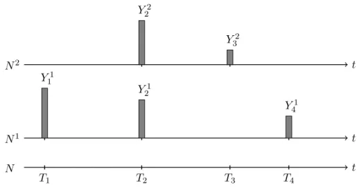
3.1 An example combining trigger events, thinning and claim sizes. . . 36

3.2 The surplus process under feedback control in infinitesimal time intervals 43 4.1 A trajectory of the filter process . . . 56

4.2 The feedback control in the reduced control problem . . . 61

4.3 The a priori bounds for the optimal reinsurance strategy . . . 94

4.4 The optimal reinsurance strategy under full information . . . 99

4.5 The effect of the risk aversion parameter on the optimal reinsurance strat-egy under full information . . . 100

4.6 The effect of the safety loading parameter of the reinsurer on the optimal reinsurance strategy under full information . . . 101

4.7 The optimal investment strategy . . . 101

4.8 The a priori bounds and two upper bounds for the optimal reinsurance strategy. . . 102

4.9 Trajectories of the surplus process in an insurance loss szenario for three different insurance strategies . . . 103

5.1 A trajectory of the filter process . . . 114

5.3 The a priori bounds and two upper bounds for the optimal reinsurance strategy depending on the accident realizations. . . 143

6.1 A trajectory of the filter process . . . 153

6.3 The a priori bounds and two upper bounds for the optimal reinsurance strategy . . . 168

(12)

(13)

List of Tables

3.1 Numerical values for the Figure 3.1 . . . 35

4.1 Simulation parameters for Section 4.9 . . . 98

(14)

(15)

Abbreviations

BSDE backward stochastic differential equation càdlàg continu à droite avec limité à gauche DPP dynamical programming principle DSPP doubly stochastic Poisson process

FTCL Fundamental Theorem of Calculus for the Lebesgue integral FV finite variation

HJB Hamilton-Jacobi-Bellman

iid independent and identically distributed LoB line of business

MPP marked point process mPP mixed Poisson process ODE ordinary differential equation PDE partial differential equation PRM Poisson random measure SDE stochastic differential equation SPP simple point process

(16)

(17)

Basic Notations

Integers and real numbers

N0 N∪ {0}, set of non-negative integers

N0 N0∪ {+∞}, set of non-negative integers including infinity

R+ [0,∞), set of non-negative real numbers

R+ [0,∞)∪ {+∞}, compactification of non-negative real numbers

Special symbols

k · k `1-norm

k · k2 Euclidean norm

δ₍_x₎ Dirac measure located at x, i.e.δ₍_x₎(A):=1A(x)

1A Indicator function of a setA

co{A} Convex hull ofA⊂_Rn

B(E) Borelσ-algebra on E

B+ _Borel_σ_{-algebra on}

R+

P(Ω) Set of all subsets of a non-empty set Ω P(F) Predictable σ-algebra of the filtrationF σ(A) σ-algebra generated by a setA

A∨B σ(A∪B),σ-algebra generated byA and B ek k-th unit vector inRm,k∈ {1, . . . , m}

∂Cf(x) Clarke’s generalized gradient, cf. Def. 2.6

f◦(x;v) Generalized directional derivative of f atx in directionv, cf. Def. 2.4 (X)c Continuous part of the process X, cf. Def. 2.49

[X] Quadratic variation process of X, cf. Def. 2.50

[X, Y] Quadratic covariation process of X and Y, cf. Def. 2.50 E(X) Dol´eans-Dade exponential ofX, cf. Def. 2.61

(18)

Special sets

Ed ₍₀_,_∞)d_{× P(}

D), mark space of the MPP Ψ = (Tn,(Yn, Zn))n∈_N

∆k (k−1)-dimensional probability simplex,k≥2

˚

∆k Interior of the probability simplex ∆k,k≥2

A(_P,F) Set of all F-adapted finite variation processes w.r.t. P, cf. Def. 2.47

M(_P,F) Set of all c`adl`ag (P,F)-martingales starting at zero, cf. Def. 2.32

M_l_oc(P,F) Set of all c`adl`ag local (P,F)-martingales starting at zero

Function spaces

AC([a, b]) Set of all absolutely continuous functions on [a, b] BV([a, b]) Set of all function of bounded variation on [a, b] Lip(I) Set of all Lipschitz function onI ⊆_Rn

(19)

Chapter 1

Introduction

1.1 Motivation and literature overview

Many challenges are currently facing the insurance industry. On the one hand, the num-ber and volume of insurance losses are growing as a result of the weather fluctuations due to climate change.1 On the other hand, the current structural low interest rate envi-ronment and higher volatility on financial markets are making it more difficult to achieve profitable investments. Further challenges arise from the transparency of insurance con-tracts provided by comparison portals, as well as the comprehensive inter-connectedness resulting from the digitalization trend and the data generated from it, which can be used to identify and record risks. For many years, questions inherited from the first two chal-lenges regarding effective strategies for reducing the insurance risk and optimal capital investment have been attracting the attention of researches in actuarial mathematics. In fact, a classical task in risk theory is to deal with optimal risk control and optimal asset allocation for an insurance company.

Generally, the risk of an insurer results from the compensation of insurance claims in exchange for regular premiums, in which an insurance claim is a request to an insurance company for a payment related to the terms of an insurance policy.2 This risk can be reduced by ceding claims to a reinsurance company in return for relinquishing part of the premium income to the reinsurer. More precisely, the reinsurer covers part of the costs of claims against the insurer. Notice that we refer to the cost of a claim as the claim size, magnitude, loss or amount of damage.

The surplus of the insurance company arises from the premiums left to the insurer after transferring the risk to the reinsurer and from the payments to be made by the insurer. This surplus is deposited in a financial market, which leads to an optimal in-vestment-reinsurance problem in continuous time under the assumption that the insurer can continuously purchase a reinsurance contract and invest in a financial market. These problems have been previously intensively studied in the literature using various opti-mization criteria, in which maximizing the utility and minimizing the ruin probability are two frequently used optimization criteria.

Schmidli [110], Promislow and Young [103] and Cao and Wan [34] employed a Black-Scholes-type financial market and proportional reinsurance (as will be done in this work) for optimal control problems. While the first two articles provide optimal investment-reinsurance strategies (a closed-form and analytical expression for the investment-reinsurance strat-egy, respectively) under the criteria of minimizing the ruin probability, the third article offers an explicit expression for the problem of maximizing the exponential utility of terminal wealth. Other articles (with other settings) that are worth mentioning are

1

See Faust and Rauch [58]. 2

See Cambridge Dict. [33].

(20)

those by Zhang and Siu [123], in which an optimization problem was formulated as a stochastic differential game between the insurer and the market; Schmidli [111], who studied several optimization problems in insurance under different frameworks; and Bai and Guo [11], who showed in some special cases the equivalence of optimal strategies for maximizing the expected exponential utility of terminal wealth and minimizing the probability of ruin.

The cited literature deals with the jump part of the surplus process, which describes the net claim process (premium income minus claim compensation), in two different ways. The first way is to use the well-known Cramér-Lundberg model from classical risk theory (see Bühlmann [15]) to describe the net claim process, as was done by Schmidli [110]. The Cramér-Lundberg model was first introduced by Filip Lundberg in his work [88] and was also named after Harald Cramér because of his basic findings with that model (see [43]). The second way is to use the diffusion approximation considered by Iglehart [70] for the jump term in the Cramér-Lundberg model, as outlined by Grandell [66, Sec. 1.2]. Hence, with such an approximation approach, the optimization problem was studied by Cao and Wan [34] and Promislow and Young [103]. Both approaches were also examined by Zhang and Siu [123] and Schmidli [111].

In all of the articles mentioned so far, the assumption of full information is used as a common feature, which means that the insurer has complete knowledge of the model parameters. However, in reality, insurance companies operate in a setting with partial information; that is, with regard to the net claim process, only the claim arrival times and magnitudes are directly observable, but the claim intensity, which is required by all net claim models, is not observable by the insurer, as pointed out by Grandell [66, Ch. 2]. In the context of financial markets, partial information means that the terms of drift and volatility are unknown, even though the term of volatility is typically assumed to be known as it can be estimated very well, whereas the appreciation rate is notoriously difficult to estimate (see Rogers [107, Sec. 4.2]).

As mentioned, insurers make decisions solely on the basis of the information at their disposal in practice. Therefore, we herein investigate the optimal investment and rein-surance problem in a partial information framework. We first emphasize that partial information control problems are different from partial observation control problems in that the controls of the latter problems are based on noisy observations of the state pro-cess. Di Nunno and Øksendal [52] were the first to study a partial information optimal portfolio problem in the sense that the dealer has access to only some information repre-sented by a filtration, which is generally smaller than the one generated by the financial market. This problem was also investigated by Liang et al. [87] in the presence of both investment and reinsurance, in what partial information refers to the financial market. In this work, we assume that full information is available on the financial market and focus on the insurance risk with an unobservable claim intensity.

On the basis of the suggestion of Albrecher and Asmussen [4, p. 165], Liang and Bayraktar [85] considered the optimal investment and reinsurance problem for maximiz-ing exponential utility under the assumption that the claim intensity and loss distribution depend on the state of a non-observable Markov chain (hidden Markov chain), which describes different environment states, whereby the net claim process is modelled as a compound Poisson process and the fully observable financial market is modelled as a Black-Scholes financial market with one risky and one risk-free asset. In this thesis, we use the same financial market model; moreover, our assumption on the claim inten-sity can be considered as a special case of one state of the above-mentioned Markovian regime-switching model; namely, we model the intensity as an unobservable random variable, which places us in a Bayesian setting. However, literature with a setting of

(21)

1.1 Motivation and literature overview 3

partial information focuses only on one line of business (LoB) to gain an optimal rein-surance strategy. However, in reality, there is often a dependency between the different risk processes of an insurance company. This results from the fact that customers of a typical insurance company have insurance policies of different types, such as building, private-liability or health insurance contracts.

A simplified example of a possible dependency between several types of risk is that of a storm event accompanied by heavy rainfall, wherein flying roof tiles cause damage to third parties and flooding leads to damage in buildings. In addition to this depen-dency between private-liability insurance and building insurance, there may even be a dependency on motor-liability insurance and health insurance if a car accident occurs as a result of adverse traffic circumstances due to that heavy rainfall. Therefore, in order to appropriately model the insurance risks of an insurer, we need to capture the dependency structure using a multivariate model.

Thinning is a commonly used approach to impose dependency between several types of insurance risks, which is also the case in this thesis. The idea of this approach is that the occurrence of claims depends on a certain process that generates events that cause damage to LoBiwith probability pi and to LoBj with probability pj, where all claims

occur simultaneously at the trigger arrival time. Therefore, these models are referred to ascommon shock risk models. An example of a shock event is the storm event described above. Typically, the corresponding claim sizes are determined independently of the appearance times.

This typical assumption is also considered to be fulfilled in this work. The thinning approach traces back to Yuen and Wang [122]. Anastasiadis and Chukova [8] provided a literature overview of multivariate insurance models from 1971 to 2008.

Another multivariate model that avoids referencing an external mechanism was given by Bäuerle and Grübel [28], who proposed a multivariate continuous Markov chain of pure birth type with inter-dependency arising from the dependency of the birth rates on the number of claims in other component processes. Scherer and Selch [108] constructed the dependency of the marginal processes of a multiple claim arrival process by introduc-ing a Lévy subordinator serving as a joint stochastic clock, which lead to a multivariate Cox process in the sense that marginal processes are univariate Cox processes.

Another frequently discussed dependency concept based on copula. Cont and Tankov [41, Ch. 5] described the dependency structure of multi-dimensional Lévy processes in terms of Lévy copula. However, as pointed out by Bäuerle and Grübel [27, p. 5], the dependency modelling for Lévy processes is reduced to the choice of thinning properties as a consequence of their defining properties. On the basis of this limitation, Bäuerle and Grübel [27] extended Lévy models by incorporating random shifts in time such that the timings of claims caused by a single trigger event are shifted according to some distribution, where some of these claims are thinned out and do not occur. Section 5.9 discusses why such shifts cannot be incorporated in this work. For further multivariate claim count models, please refer to the literature cited by Scherer and Selch [108, Sec. 1.3]. In connection with optimal reinsurance problems, a Lévy approach was discussed by Bäuerle and Blatter [25]. They showed that constant investment and reinsurance (pro-portional reinsurance as well as a mixture of pro(pro-portional and excess-of-loss reinsurance) is the optimal strategy for maximizing the exponential utility of terminal wealth.

In addition to the L´evy model, optimization problems with common shock models have been investigated by Centeno [37], who studied optimal excess-of-loss retention limits for a bivariate compound Poisson risk model in a static setting. The corresponding dynamic model was used by Bai et al. [10] to derive optimal excess-of-loss reinsurance policies (which turned out to be constant) under the criterion of minimizing the ruin probability

(22)

by making use of a diffusion approximation. For the same model, Liang and Yuen [86] derived a closed-form expression for the optimal proportional reinsurance strategy of the exponential utility maximizing problem both with and without diffusion approximation using the variance premium principle. Bi and Chen [16] also investigated the same problem with the expected value premium principle in the presence of a Black-Scholes financial market. In the case of an insurance company with more than two LoBs, Yuen et al. [121] and Wei et al. [117] sought optimal proportional reinsurance to maximize the exponential utility of terminal wealth and the adjustment coefficient, respectively, in which the strategies are only stated for two LoBs. However, all optimization problems with multivariate insurance models are considered under full information.

In this work, we will describe the dependency structure between different LoBs using the thinning approach while dealing with unobservable thinning probabilities. To our knowledge, this is the first time an optimal reinsurance and investment problem under partial information using a multivariate claim arrival model with possibly dependent marginal processes is studied. In order to solve this optimal control problem, the dy-namic programming Hamilton-Jacobi-Bellman (HJB) approach will be applied, which is the most widely used method for stochastic control problems. The HJB equation is a classical tool for deriving optimal strategies for control problems. This equation can be obtained by applying the dynamic programming principle, which was pioneered by Richard Bellman, after whom the HJB equation is named, in the 1950s (see [13, 14]). In classical physics, the diffusion case of this equation can be viewed as an extended Hamilton-Jacobi equation, which was named after William Rowan Hamilton and Carl Gustav Jacob Jacobi.3

The HJB equation is a deterministic (integro-) partial differential equation whose solution is the value function of the corresponding stochastic control problem under certain conditions. However, in general, the existence of a solution to this equation is not guaranteed because of smoothness requirements of the solution. In our setting, we will have to deal with the strong assumption of differentiability of the value function, which cannot be guaranteed. Over the past decades, a rich theory has been developed to overcome this difficulty. In the early 1980s, Pierre-Louis Lions and Michael Crandall introduced the currently popular concept known as theviscosity solution for non-linear first-order partial differential equations (see [45]), which claims that the value function is the unique viscosity solution to the HJB equation under mild conditions (continuity and, in more general frameworks, even discontinuity).4 The basic idea behind this concept is to estimate the value function from above and below using smooth test functions. Fleming and Soner [61] applied the viscosity approach to optimise the control of Markov processes.

Another approach is to generalize the HJB equation by including Clarke’s generalized gradient, which is a weaker notation of differentiability. Clarke [39] and Davis [47] came up with this idea which the strong assumption of differentiability of the value function can be weakened to local Lipschitz continuity. The generalization concept of the HJB equation has been applied in an article by Liang and Bayraktar [85] and is also used in this work.

As indicated above, we consider the surplus process of an insurance company with various LoBs in which claim arrivals are modelled using a common shock model under incomplete information (i.e. the claim intensity and the thinning probabilities are un-known to the insurer). Our aim is to solve the optimization problem facing insurance

3

See Section 5.1.2 in Blatter [17] and Section 9.1 in Popp [102]. 4

For a historical survey for the development of the viscosity solution, we refer the reader to Yong and Zhou [120, Sec. 4.1] and Fleming and Soner [61, Sec. II.17].

(23)

1.2 Main results and outline 5

companies by trying to find investment-reinsurance strategies that maximizes the ex-pected exponential utility of terminal wealth. Using a Bayesian approach, we overcome the issue of uncertainty and obtain a reduced control problem, which is investigated with the help of the dynamic programming principle and a generalized HJB equation. Before entering the world of our insurance model, let us introduce the outline of the thesis and highlight the main results.

1.2 Main results and outline

In this thesis, we deal with a multi-dimensional insurance risk model. The main aim here is to study the impact of partial information regarding the inter-dependencies be-tween marginal risk processes on the optimal investment and proportional reinsurance under the criterion of maximizing the expected exponential utility of terminal wealth. Preparing for the introduction of the risk model and the solution technique of the corre-sponding control problem, Chapter 2 is dedicated to the fundamentals, starting with the concept of Clarke’s generalized gradient in Section 2.1. After providing a brief overview of the basic definitions and properties of stochastic processes in Section 2.2, we recall some important tools of stochastic analysis in Section 2.3. This is then followed by Sec-tion 2.4, which is devoted to the (marked) point processes used for modelling the net claim process. Section 2.4.1 includes basic definitions and notations, and Section 2.4.2 deals with the concept of the intensities of point processes, our main object of interest for the characterization of point processes. This concept is generalized in Section 2.4.4 to marked point processes. In Sections 2.4.3 and 2.4.5, we proceed with the study of the innovation method for filtering with point and marked point process observations, respectively, in a simplified setting, which is sufficient for the following chapters.

Following this introductory chapter, we introduce a control problem under partial information in Chapter 3. For this purpose, we specify the multivariate claim arrival model in Section 3.1 as a common shock model, in which the shock generating intensity (background intensity) and the thinning probabilities describing the affected LoBs are unobservable, which is considered by modelling these parameters as random variables. Moreover, we also model the claim size distribution as unknown. In contrast to the cited literature considering optimal reinsurance problems in a multivariate setting, the reinsurance strategies of different LoBs are supposed to be equal in our work, which is equivalent to the assumption of one reinsurance policy for an entire insurance company. In Section 4.10, we discuss the consequences of various reinsurance contracts. Further-more, as the focus is on the optimal reinsurance strategy, we use a quite simple financial market model with one risk-free and one risky asset modelled as geometric Brownian mo-tion, which is presented in Section 3.2. Subsequently, we introduce investment strategies (see Section 3.3), proportional reinsurance strategies (see Section 4.3) and a reinsurance premium principle (see Section 3.5). This results in the definition of the surplus process in Section 3.6, the basic object of interest in the stochastic control problem under par-tial information stated in Section 3.7. The next three chapters address the incomplete information problem under different assumptions for unknown parameters.

For the sake of simplicity, we restrict ourselves to the study of the case of an observable background intensity and claim size distribution in Chapter 4. This case is specified in Section 4.1, where we suppose that the vector of thinning probabilities takes values in a finite set. In order to overcome the difficulty of partial information in thinning probabilities, we determine an observable estimator of these probabilities by means of filtering theory for marked point process observations in Section 4.2. With the help of the

(24)

derived filter, we formulate a reduced control model and problem in Section 4.3, for which we derive the generalized HJB equation in Section 4.4 by replacing the partial derivative with respect to time by the corresponding Clarke’s generalized subdifferential, which is introduced in Section 2.1. We then receive candidates for an optimal investment and reinsurance strategy in Sections 4.5 and 4.6. It then turns out that the candidate for the optimal investment strategy is deterministic, in particular independent of the reinsurance strategy, whereas the unique candidate for the optimal reinsurance strategy depends not only on the safety loading parameter of reinsurance and time, but also on the background intensity, claim size distribution and the filter process. In Section 4.7, we continue with the verification procedure by showing that a solution to the HJB equation does indeed coincide with the value function and that the derived candidates for the optimal strategies are indeed optimal. Afterwards, we prove the existence of a solution to the HJB equation. Section 4.8 includes a comparative result of the optimal reinsurance strategy under full information with the one under partial information, in which we suppose identical claim size distributions for every LoB. We find that the optimal reinsurance strategy in the multivariate risk model with known thinning probabilities is always greater than or equal to the one in the risk model with unknown thinning probabilities. The comparison result is illustrated in Section 4.9. We close the chapter with a discussion on the generalizations of the setting used in this chapter, particularly concerning the thinning probabilities.

In Chapter 5 we investigate the partial information problem under the assumptions of observable claim size distribution, unobservable background intensity taking values in a finite set and Dirichlet distributed thinning probabilities (see Section 5.1). Using a filter as an estimator for the background intensity and the conjugated property of the Dirichlet distribution, we proceed as in the previous chapter by stating the reduced control problem (see Section 5.3) and the corresponding generalized HJB equation, in which we need to replace partial derivatives with respect to time and the components of the filter for the background intensity by the corresponding Clarke’s generalized gradient. The HJB equation yields the same optimal investment strategy as in Chapter 4, and the optimal reinsurance strategy has a similar structure. The verification step runs as before (see Section 5.6) and shows the optimality of the proposed investment-reinsurance strategy. In Section 5.7, we provide a comparison result similar to the one in the previous chapter, again under the assumption of identical claim size distributions for all insurance classes, which is visualized in Section 5.8. Finally, some generalizations of the setting of this chapter and resulting difficulties regarding the used solution technique are discussed. Chapter 6 is devoted to the case of an unobservable claim size distribution for the introduced control problem under partial information, in which the framework is quite simple as a result of supposing that there are only a finite number of potential claim size distributions. Section 6.9 establishes the difficulties faced with more general settings. In order to simplify the optimality analysis, we consider working on the insurance model with one LoB and observable background intensity (see Section 6.1), with the result being a similarly optimal investment-reinsurance strategy and correspondingly analogous verification. Moreover, we develop a similar comparative result as before, which yields a very small range of possible optimal reinsurance strategies for some scenarios in the numerical study in Section 6.8.

Appendix A includes auxiliary results for the verification procedure in Chapters 4, 5 and 6, and some useful inequalities are covered in Appendix B.

(25)

Chapter 2

Fundamentals

Before getting into the detail of our insurance model and the optimization problem, let us recall some foundations of stochastic processes and filter results with (marked) point process observations to make this work self-contained.

2.1 Clarke’s generalized gradient

We start this chapter by briefly introducing a concept of nonsmooth analysis, namely Clarke’s generalized gradient, which was introduced by Clarke [39, Ch. 2]. We consider only the case of functions defined on the Euclidean space (Rn,k · k2) equipped with the

Euclidean normk · k2 instead of a general Banach space.

Notation. Let r > 0 some scalar and x ∈_Rn _{some vector. We denote the open ball of}

radiusr about x by Br(x):={y∈Rn:kx−yk< r}.

Definition 2.1([39], p. 25; [115], Def. 4.6.9; Lipschitz function). LetI ⊂Rnbe a subset

ofRn and f :I →R be a function defined onI.

(i) We say f isLipschitz on I (of rank K) or satisfies a Lipschitz condition on I (of rank K) if there exists 0< K <∞ such that

|f(x1)−f(x2)| ≤Kkx1−x2k2

for all x1, x2 ∈I.

(ii) The function f is said to be Lipschitz (of rank K) near x ∈ I if there exists ε =ε(x) >0 such that f is Lipschitz onI ∩Bε(x). Iff is Lipschitz (of rank K)

near x for allx∈I, then we say f islocally Lipschitz onI (of rank K).

We writeLip(I) for the set of all Lipschitz function onI andLip_l_oc(I) for the collection of all locally Lipschitz function onI.

A useful result is that every convex function defined on an open convex set is locally Lipschitz.

Theorem 2.2 ([106], Thm. A). Let f be convex on an open convex set I ⊆Rn. Then

f ∈Lip_l_oc(I) and, consequently, f ∈Lip(C) for all compact sets C ⊂I.

Let us mention further result of Lipschitz functions.

Theorem 2.3 ([40], Thm. 3.4.1, Remark 3.4.2; Rademacher’s Theorem). Let I ⊆_Rn _be a subset andf ∈Lip_l_oc(I). Thenf is differentiable almost everywhere on I in the sense of the Lebesgue measure.

(26)

To define Clarke’s generalized gradient, we must first introduce the generalized direc-tional derivation.

Definition 2.4 ([39], p. 25). Let x ∈ _Rn _{be a given point and} _v _∈

Rn be some other

vector. Moreover, letf be Lipschitz near x. Then thegeneralized directional derivative

of f atx in the directionv, denoted byf◦(x;v), is defined by

f◦(x;v) = lim sup

y→x h↓0

f(y+h v)−f(y)

h .

Justification of the definition. Due to the locally Lipschitz property of f, the difference quotient is bounded above by Kkvk₂ for some 0< K < ∞ and for y sufficient near x as well as h sufficient near 0. Therefore,f◦(x;v) is well-defined since the upper limit is taken from the bounded difference quotient and no limit is presupposed.

Beside the finite property, the generalized directional derivative admits the following elementary properties.

Proposition 2.5([39], Prop. 2.1.1). Letf be Lipschitz nearx∈_Rn_{. Then}_v_7→_f◦₍_x_;_v₎ is positively homogeneous and subadditive.

These properties justifies the existence of the next defined generalized gradient. On account of the Hahn-Banach Theorem, we know that any positively homogeneous and subadditive functional onRnmajorizes some linear functional onRn. Consequently, the

proposition above implies the existence of at least one linear functional ξ : Rn → R

with f◦(x;v) ≥ ξ(v). It therefore follows by ξ(v) ≤ Kkvk2 for some 0 < K < ∞

that ξ belongs to the dual space of Rn of continuous linear functionals on Rn. Clarke’s

generalized gradient will be defined as a subset of the continuous linear functionals and thus is non-empty by the explanation above. Since a continuously linear functionalξ on

Rncan be identified byξ ∈Rn, the generalized gradient is a subset ofRnin our setting.

Definition 2.6 ([39], p. 27). Letf be Lipschitz nearx∈_Rn_{. Then}_{Clarke’s generalized} gradient (generalized gradient for short) of f atx, denoted by∂Cf(x), is given by

∂Cf(x):=

ξ ∈_Rn:f◦(x;v)≥ξ>v∀v∈_Rn .

In the univariate case we call ∂Cf(x) Clarke’s generalized subdifferential (generalized subdifferential for short) of f atx.

We continue with properties of the generalized gradient.

Proposition 2.7 ([39], Prop. 2.1.2). Let f be Lipschitz near x∈_Rn_{. Then} _∂C_f₍_x₎ _{is a} convex and compact subset of Rn.

Proposition 2.8 ([39], Prop. 2.2.4). If f is strictly differentiable at x ∈ _Rn _such that some differential operator D is defined, then f is Lipschitz near x and ∂Cf(x) = {Df(x)}. Conversely, if f is Lipschitz near x and ∂Cf(x) reduces to a singleton {ξ}, thenf is strictly differentiable at x and Df(x) =ξ.

The next characterization of Clarke’s generalized gradient will be needed to show existence of a solution of the generalized HJB equation (cf. Theorems 4.33, 5.26 and 6.17) since it allows us to reduce the case of non-differentiability to the case of differentiability.

(27)

2.2 Stochastic processes 9

Theorem 2.9 ([39], Thm. 2.5.1). Let f be Lipschitz nearx∈_Rn_, _Ω

f the set of points at which the function f is not differentiable andS an arbitrary set of Lebesgue-measure

0 in Rn. Then ∂Cf(x) = co n lim n→∞∇f(xn) :xn→x, xn∈/ S, xn∈/Ωf o ,

where co{A} denotes the convex hull of A⊂_Rn_.

2.2 Stochastic processes

We start this chapter with briefly recalling some general definitions and results about stochastic processes cited from Karatzas and Shreve [73, Ch. 1], Protter [104, Ch. 1, 2], Capasso and Bakstein [35, Sec. 2.1], Elstrodt [56, Sec. II.6], Bain and Crisan [12, Sec. A.5], Klebaner [75, Ch. 8] and Chung and Williams [38, Ch. 2], which will be of importance in the following proceedings. Throughout this chapter all stochastic quantities are defined on a fixed probability space (Ω,F,P).

Recall that astochastic processXon (Ω,F,P) is a family ofRd-valued random variable

(Xt)t≥0 for d ∈ N. For the sake of convenience, we will use the shorter term process

instead of stochastic process. A process can be seen as a function X : R+×Ω → Rd

whereX(t,·) =Xt is an F-measurable random variable for all t≥0. For a fixed ω∈Ω,

the mappingt7→Xt(ω) fromR+ intoRis called a sample path ortrajectory of X.

For two processesXandY, the notationX > Y meansXt(ω)> Yt(ω) for allt≥0 and

all ω∈Ω. In particular, X≥0 stands for Xt(ω)≥0 for all ω∈Ω andt≥0. Similarly,

we use the notationsX ≥Y,X < Y,X ≤Y andX =Y. Furthermore, we sayXandY are the same if and only ifX=Y. As we know null sets are normally overlooked in the present of probability measures. Accordingly, we introduce in the following alternative concepts of “equality”.

Definition 2.10([73], Def. 1.1.2, Def. 1.1.3). LetXand Y be two processes. ThenY is called amodification orversion of X if P(Xt=Yt) = 1 for all t≥0. IfP(Xt =Yt, t≥

0) = 1, then X and Y are said to beindistinguishable.

Remark 2.11 ([104], p. 4). The sample paths of indistinguishable processes differ only on a P-null set, which does not hold for modifications in general since the uncountable

union of null sets can have any probability between 0 and 1, and it can even be non-measurable.

Convention. We say that an equation with functions of processes on both sides (e.g. evo-lution equations for processes)holds up to indistinguishability if the processes described by the both sides of the equality are indistinguishable.

Next, we move on to some regularity properties of sample paths, which are defined for almost allω since indistinguishable processes are regarded as equal.

Definition 2.12. A process X = (Xt)t≥0 is called continuous if lims→tXs(ω) =Xt(ω)

for all t≥0 and P-almost all ω ∈ Ω. Moreover, X is said to be right-continuous ( left-continuous) if lims↓tXs(ω) = Xt(ω) (lims↑tXs(ω) = Xt(ω)) for all t ≥ 0 (t > 0) and P-almost all ω ∈ Ω. Furthermore, X is called c`adl`ag if it is right-continuous and the

left-hand limit lims↑tXs(ω) exists for allt >0 and P-almost allω∈Ω. IfX is c`adl`ag,

then the process X− = (Xt−)t≥0 defined by X0− := 0, Xt− := lims↑tXs for all t >0 is

said to be theleft-hand limit process ofX, and the process ∆X= (∆Xt)t≥0 defined by

(28)

Lemma 2.13 ([12], Lem. A.14). Let X = (Xt)t≥0 be a c`adl`ag process. Then {t ≥ 0 :

P(Xt−6=Xt)>0} contains at most countably many points.

Proposition 2.14 ([104], Thm. I.2). Let X andY be two processes where Y is a modi-fication of X. If X and Y have right-continuous sample paths P-almost surely, then X and Y are indistinguishable.

Definition 2.15 ([73], Def. 1.1.6; Measurability). A processX= (Xt)t≥0 is called

mea-surable w.r.t. F if the mapping (t, ω) 7→ Xt(ω) : R+ ×Ω,B+⊗ F → R,B(R) is

measurable, i.e. {(t, ω)∈_R₊×Ω :Xt(ω)∈B, B ∈ B(R)} ∈ B+⊗ F.

Proposition 2.16. If the processX = (Xt)t≥0 is either left- or right-continuous, then

X is measurable.

Proposition 2.17. IfX= (Xt)t≥0 is a measurable process, then the sample pathX·(ω) : R+→R isB+-measurable for all ω∈Ω.

Another important notion in the context of stochastic processes is the filtration. In insurance mathematics, filtrations are used to model the available information for the in-surer. Especially for the models with partial information, the measurability of processes w.r.t. different filtration processes is an important aspect.

Definition 2.18 ([73], p. 3 ff.). A family ofσ-algebras F= (F_t)t≥0 with Ft⊂ F for all

t≥0 is called afiltration ifFs ⊂ Ftfor all 0≤s≤t. We set F∞:=σ S_t_≥₀Ft

. For a filtrationF= (Ft)t≥0, we define by Ft+ :=T_s>tFs theσ-algebra of events immediately after t ≥ 0 and by F_t− := σ S_s<tFs

the σ-algebra of events strictly prior to t ≥ 0, whereF0− := 0. We say the filtrationF= (Ft)t≥0 isright-(left-)continuous ifFt=Ft+

(resp.Ft=Ft−) for allt≥0. The probability space (Ω,F,P) equipped with a filtration

F, denoted by (Ω,F,F= (F_t)t≥0,P), is called a filtrated probability space.

Notation. To shorten notation we write in the followingF to denote F= (Ft)t≥0.

Definition 2.19 ([73], Def. 1.1.9; Adaption). A process X = (Xt)t≥0 defined on a

filtrated probability space (Ω,F,F,P) is called F-adapted if Xt is Ft-measurable for

each t≥0.

Definition 2.20 ([104], p. 16; Natural filtration). For a process X = (Xt)t≥0, the

fil-tration FX = (FX

t )t≥0 defined by FtX := σ(Xs : 0 ≤ s ≤ t) is said to be the natural filtration of X.

So the natural filtration FX is the smallest filtration making X adapted. It should be noted that the following two statements do not hold in general: 1. FX

0 contains all

P-null sets ofF; 2. FX is right-continuous. However these two statements are important

technical assumptions for numerous results involving stochastic processes. So filtrations are usually modified as shown below to meet these technical requirements.

Definition 2.21 ([56], Def. 6.1). A probability space (Ω,F,P) is called complete if for

all A⊂B ∈ F withP(B) = 0 implies thatA∈ F.

The assumption of a complete probability space is not a restriction since for any probability space there exists a unique one which is complete.

(29)

Proposition 2.22 ([56], Thm. 6.3). Let (Ω,F,P) be a probability space and

N :={A⊂N :N ∈ F,P(N) = 0},

e

F :={A∪N :A∈ F, N ∈ N }, e

P:F →e [0,1], eP(A∪N):=P(A) for A∈ F, N ∈ N.

Then Fe is a σ-algebra, e_P is well-defined and (Ω,Fe,_Pe) is a complete probability space.

Futhermore,Fe is the smallestσ-algebra such that (Ω,Fe,Pe) is complete.

Definition 2.23 ([56], p. 64). The probability measure e_P in Proposition 2.22 is called a completion of P and the probability space (Ω,Fe,Pe) in Proposition 2.22 is called a

completion of (Ω,F,P).

Definition 2.24 ([104], p. 3). A filtered probability space (Ω,F,F,P) is said to satisfy

theusual conditions if

(i) the probability space (Ω,F,P) is complete,

(ii) F₀ contains all P-null sets ofF,

(iii) Fis right-continuous.

Remark 2.25. Proposition 2.22 has shown that for any probability space there exists a unique completion. A complete probability space (Ω,F,P) equipped with the filtrationF

can be enlarged to a filtrated probability space (Ω,F,F,e P) satisfying the usual conditions by e Ft:= \ s>t σ(Fs,N) with N :={A∈ F :P(A) = 0}.

Obviously,Fe_t=Fe_t₊ for allt≥0 andFe₀ contains allP-null sets ofF. Therefore, for any given filtrated probability space, we can easily find one holding the usual conditions.

In the following, we assume that (Ω,F,F,P) is a filtrated probability space satisfying the usual conditions.

We continue by introducing a stricter concept of measurability than in Definition 2.15.

Definition 2.26 ([73], Def. 1.1.11; Progessiv measurability). A process X = (Xt)t≥0

is called an F-progressive process or an F-progressively measurable if (s, ω) 7→ Xs(ω) :

([0, t]×Ω,B([0, t])⊗ F_t) → (R,B(R)) is B([0, t])⊗ Ft-measurable for all t ≥ 0, i.e.

{(s, ω)∈[0, t]×Ω :Xs(ω)∈B, B∈ B(R)} ∈ B([0, t])⊗ Ft for allt≥0.

Proposition 2.27. If a process X = (Xt)t≥0 is F-progressively measurable, then X is

measurable and F-adapted.

Proof. Fixt≥0 andB ∈ B(_R). From Definition 2.26 follows directly that {Xs∈B} ∈

F_tfor alls∈[0, t] and, in particular,{Xt∈B} ∈ Ft, which means thatXisF-adapted.

Another consequence of Definition 2.26 is that {(s, ω) ∈ [0, n]×Ω : Xs(ω) ∈ B} ∈

B([0, n])⊗ Ft ⊂ B+⊗ F for all n ∈ N. Hence X1[0,n]×Ω is measurable w.r.t. F and,

consequently,X= limn→∞X1Ω×[0,n] as well.

Proposition 2.28 ([73], Prop. 1.1.12). Let X = (Xt)t≥0 be measurable w.r.t. F and

F-adapted. Then X has an F-progressively measurable modification.

Proposition 2.29 ([73], Prop. 1.1.13). If a process X = (Xt)t≥0 is F-adapted and

(30)

Lemma 2.30. Let X = (Xt)t≥0 be a non-negative F-progressive process. Then the

process (Rt

0 Xsds)t≥0 is F-adapted.

Proof. The proof is given in Br´emaud [20], solution of Exercise E10 on page 53.

Proposition 2.31([79], Lemma 1.1 (a)). Let(E,E)be a measurable space, where E is a complete separable metric space. Let X = (Xt)t≥0 be a c`adl`ag E-valued process defined

on a filtrated probability space (Ω,F,F,P) satisfying the usual conditions. Furthermore, let G = (Gt)t≥0 be a right-continuous filtration such that Gt contains all P-null sets of

(Ω,F) andGt⊂ Ft for all t≥0. Then there exists a c`adl`ag modification of the process

(E[f(Xt)| Gt])t≥0 for all measurable bounded functions f defined on E.

Let us recall the basic concept of (local) martingals.

Definition 2.32 ([104], p. 7; Martingale). An F-adapted process M = (Mt)t≥0 with

E[|Mt|]<∞ for all t≥0 is called (P,F)-martingale ifE[Mt|Fs] =Ms for all 0≤s < t.

If the equation is weakened to E[Mt|Fs] ≥ Ms (E[Mt|Fs] ≤ Ms) for every 0 ≤ s < t,

thenM is said to be a (P,F)-submartingale ((P,F)-supermartingale).

Convention. If it is clear that the underlying probability measure isP, then we omit P

in the appellation (P,F)-martingale and write only F-martingale. A similar convention

applies to all subsequent definitions, in which a probability measure appears.

Notation. M(P,F) denotes the set of all c`adl`ag (P,F)-martingales starting at zero.

Definition 2.33. Let 0< C < ∞ be some constant. A process X = (Xt)t≥0 is called

bounded byC if sup_t≥0|Xt|< C P-a.s.

Proposition 2.34 ([77], Rem. 21.68). A bounded local martingale is a martingale.

For the definition of local martingales let us recall the notion of stopping time.

Definition 2.35 (Stopping time). An F-measurable function τ : Ω → [0,∞] is called an F-stopping time if {τ ≤t} ∈ F_tfor all t∈[0,∞].

Proposition 2.36 ([104], Thm. I.1). Let τ : Ω→ [0,∞] be an F-measurable function. Then τ is anF-stopping time if and only if {τ < t} ∈ F_t for all t∈[0,∞].

Definition 2.37 ([104], p. 4). LetX= (Xt)t≥0 be a real-valued process andA∈ B(R).

Then τ defined byτ(ω) = inf{t >0 :Xt∈A} is called the hitting time ofA forX.

Proposition 2.38 ([104], Thm. I.3, Thm. I.4). Let X be a real-valuedF-adapted c`adl`ag process and A an open set or a closed set subset of R. Then a hitting time of A for X is an F-stopping time.

Definition 2.39. A stopping timeτ is calledfinite ifP(τ <∞) = 1.

The next defined σ-algebra contains the knowledge included in a filtration up to a stopping time.

Definition 2.40 ([104], p. 5). Letτ be a finiteF-stopping time. Then F_τ :={A∈ F :A∩ {τ ≤t} ∈ F_t, t≥0} is said to be the stopped timeσ-algebra.

(31)

Definition 2.41. Let C be a class of F-adapted processes. ThenX is called alocal C-process if there exists a non-decreasing sequence of F-stopping times (τn)n∈_N such that P(τn↑ ∞) = 1 as n→ ∞ and Xτn = (Xtτn)t≥0∈ C for eachn∈N, whereXtτn :=Xt∧τn. We writeX∈ C_l_oc. The sequence (τn)n∈_N is called alocalizing sequence forX.

In accordance with the definition, the set Mloc(F) denotes the set of local c`adl`ag F

-martingales that occurs in the definition of a semimartingale. For this definition we have to recall functions of bounded variation.

Definition 2.42 ([38], p. 75; Partition). A finite ordered set πn[a, b]:={t0, t1, . . . , tn}

forn∈_N0 such thata=t0< t1<· · ·< tn=bis called apartition of [a, b].

Definition 2.43([80], p. 421, [115], Def. 7.6.1; Bounded variation). Letf be a function defined on [a, b]. Thetotal variation function of f is defined by

V_ab(f):= sup πn_[_a,b_] ( _n X i=1 |f(ti)−f(ti−1)| ) . (2.1)

Then the numberV_ab(f) is calledtotal variation of f on [a, b]. If V_ab(f)<∞, we sayf is of bounded variation on [a, b]. The set of all functions of bounded variation on [a, b] is denoted byBV([a, b]). Letf now be defined on R+. If V0t(f)<∞ for all t≥0, then

f is said to be oflocally bounded variation on R+. In the case supt>0V0t(f) <∞, f is

calledof bounded variation on R+.

Proposition 2.44 ([115], Cor. 11.5.10). Let f : [a, b] → R be a function of bounded variation. Then f is differentiable almost everywhere (in the sense of the Lebesgue measure).

A subclass of functions of bounded variation are absolute continuous functions.

Definition 2.45 ([115], Def. 11.5.12). A function f : [a, b]→ _Ris said to be absolutely continuous if for every ε > 0 there is a δ > 0 such that given any finite sequence (Ik)i=1,...,n of pairwise disjoint open intervalsIk:= (ak, bk)⊂[a, b], we have

n X i=1 (bk−ak)< δ⇒ n X i=1 |f(bk)−f(ak)|< ε.

We writeAC([a, b]) for the set of all absolutely continuous functions on [a, b].

Lemma 2.46 ([115], Lemma 11.5.14). We have Lip([a, b])⊂AC([a, b])⊂BV([a, b]).

Next we introduce a class of processes with a strong path regularity property.

Definition 2.47 (Protter [104], p. 101; FV process). An F-adapted c`adl`ag processA= (At)t≥0 withA0 = 0 is said to be afinite variation process (FV process for short) w.r.t.

Pift7→At(ω) is of locally bounded variation on R+ forP-almost all ω∈Ω.

Notation. From now on, we write A(_P,F) for the set of all F-adapted finite variation processes w.r.t.P.

Definition 2.48 ([104], p. 102). An F-adapted c`adl`ag process Y = (Yt)t≥0 is called a

(P,F)-semimartingale if there exists a decomposition of the form

Yt=Y0+Mt+At, t≥0, (2.2)

(32)

Definition 2.49 (Continuous part). Let X = (Xt)t≥0 be an F-semimartingale. Then

process (X)c_{= ((}_X₎c

t)t≥0 denotes thecontinuous part of the process X starting at zero,

i.e.

(X)c_t =Xt−

X

0<s≤t

∆Xs−X0, t≥0.

A description of the behaviour of stochastic processes is provided by the quadratic variation.

Definition 2.50 ([75], p. 218). Let X and Y be two (P,F)-semimartingales. The quadratic covariation process of X and Y, denoted by [X, Y] = ([X, Y]t)t≥0, is defined

by [X, Y]t:= lim n−1 X i=0 Xtn i+1−Xtni Ytn i+1−Ytni , t≥0,

where the limit is understood as the limit in probability and is taken over shrinking partitions (tn_i)i of the interval [0, t] when δn= maxi(tni+1−tni)→0. The process [X, Y]

is also known as thesquare bracket process. Thequadratic variation processX, denoted by [X] = ([X]t)t≥0, is defined by [X]t= [X, X]t for allt≥0.

Notice that the existence of the quadratic covariation can be shown. Other fundamen-tal properties are summarized in the next proposition which are cited from Klebaner [75, p. 218 ff.] as well as Protter [104, p. 66 ff.].

Proposition 2.51. For two (P,F)-semimartingales X and Y the following statements are satisfied:

(i) [X, Y]is a c`adl`ag F-adapted FV process. (ii) [X, Y]is bilinear and symmetric.

(iii) [X, Y] = 1₂ [X+Y]−[X]−[Y] (polarization identity).

(iv) If one of the processes X or Y is an FV process: [X, Y]t =P0<s≤t∆Xs∆Ys for every t≥0.

(v) [X]c= [Xc].

(vi) For any t≥0, [X]t= [X]ct+X02+

P 0<s≤t(∆Xs)2. (vii) [X, Y]t=XtYt− Rt 0Xs−dYs− Rt 0Ys−Xs for all t≥0.

(viii) For any t ≥ 0, R₀·HsdXs,

R·

0KsdYs

t =

Rt

0HsKsd[X, Y]s for all F-predictable

processes (Ht)t≥0, (Kt)t≥0, where the stochastic integrals exist.

We continue with the notion of predictability, which is an integral part of studying processes in the present of jumps. An process describing the wealth of an insurances company is an example for a process with jumps occurring as a result of insurance pay-ments. Since the wealth process of an insurer is the main objection of our optimization problem, we have to deal with the notion of predictable processes.

Definition 2.52 ([38], p. 25). Let F = (F_t)t≥0 be a filtration. The family R(F) of

subsets ofR+×Ω, defined by

R(F):=

{0} ×F0:F0 ∈ F0 ∪

(s, t]×F :F ∈ F_s,0≤s < t ,

(33)

2.3 Tools of stochastic analysis 15

Definition 2.53 ([38], p. 25). The σ-algebra P(F) on R+×Ω generated by the class

of predictable rectangles P(F) :=σ(R(F)) is called F-predictable σ-algebra. A function X:R+×Ω→R is said to beF-predictable (F-previsible) ifX is P(F)-measurable.

Theorem 2.54([75], p. 213). AnF-adapted left-continuous process isP(F)-measurable.

Example 2.55. Let X be an F-adapted and c`adl`ag process. Clearly, the left-hand limit process X− is left-continuous as well as F-adapted by assumption. Hence X− is

F-predictable by Theorem 2.54.

Proposition 2.56([104], p. 103). EveryF-predictable processX isF-progressively mea-surable.

After this short overview of some basics of stochastic processes, we can now turn to some important tools of stochastic analysis, which will be intensively used in the analysis of optimization problems.

2.3 Tools of stochastic analysis

Throughout this section, we suppose that all stochastic quantities are defined on the filtrated probability space (Ω,F,F,P) satisfying the usual conditions, see Definition 2.24.

We begin this section with probably the best known formula of stochastic calculus, the Itô-Doeblin formula named after the Japanese Kiyoshi Itô, who is well-known as one of the developers of the formula, and the French Wolfgang Doeblin, who as soldier during the World War II developed a comparable formula to the other one from Itô. The famous Itô-Doeblin formula is hereafter formulated in the version for general semimartingals. For a treatment of integration w.r.t. general semimartingales we refer the reader to Protter [104] and Klebaner [75]. It should be noted that we use the following notation.

Notation. Throughout this work, we use the Riemann integral notation for integrals w.r.t. the Lebesgue measureλ, i.e. we write

Z b a g(s) dsinstead of Z [a,b] g(s)λ(ds), a < b,

for any Borel measurable function g.

Theorem 2.57([104], Thm. II.32; Itˆo-Doeblin formula). Letd≥2, Dbe an open subset of Rd and f ∈ C1,2(R+×D) be a real valued function. Furthermore, let X = (Xt)t≥0

be anD-valued F-semimartingale. Thenf(t, X) = (f(t, Xt))t≥0 is an F-semimartingale

holding f(t, Xt)−f(0, X0) = Z t 0 ft(s, Xs) ds+ d X i=1 Z t 0 fxi(s, Xs−) dX i s +1 2 d X i,j=1 Z t 0 fxixj(s, Xs−) d[X i_{, X}j_]c s + X 0<s≤t f(s, Xs)−f(s, Xs−)− d X i=1 fxi(s, Xs−)∆X i s , t≥0.

In this work the following version of the Itˆo-Doeblin formula is applied frequently, which follows immediately from the definition of the continuous part of the process X given in Definition 2.48.

(34)

Corollary 2.58. Let the conditions of Theorem 2.57 be satisfied. Then f(t, X) = (f(t, Xt))t≥0 is an F-semimartingale holding f(t, Xt)−f(0, X0) = Z t 0 ft(s, Xs) ds+ d X i=1 Z t 0 fxi(s, Xs−) d(X i₎c s +1 2 d X i,j=1 Z t 0 fxixj(s, Xs−) d[X i_{, X}j_]c s + X 0<s≤t f(s, Xs)−f(s, Xs−) , t≥0.

Theorem 2.59 ([104], p. 83; Integration by Parts, Product Rule). LetX = (Xt)t≥0 and

Y = (Yt)t≥0 be two F-semimartingales. Then (XtYt)t≥0 is an F-semimartingale holding

XtYt−X0Y0= Z t 0 Xs−dYs+ Z t 0 Ys−dXs+ [X, Y]t, t≥0.

Theorem 2.60 ([75], Thm. 8.33, Protter [104], Thm. II.37). Let X = (Xt)t≥0 be an F

-semimartingale. Then there exists an unique (up to indistinguishability)F-semimartingale

Z = (Zt)t≥0 that satisfies the stochastic differential equation (SDE for short)

dZt=Zt−dXt, Z0= 1, t≥0, where Z is given by Zt=E(X)t:=eXt−X0− 1 2[X] c t Y 0<s≤t (1 + ∆Xs)e−∆Xs, t≥0, where the infinite product converges.

Definition 2.61. The process E(X) = (E(X)t)t≥0 defined in the previous theorem is

called the stochastic exponential or theDol´eans-Dade exponential ofX.

2.4 Simple point processes and marked point processes

In this section we review some standard facts on (marked) point processes, in particular filter results, based on Br´emaud [20], Last and Brandt [80], Jacobsen [71] and Leimcke [82, Ch. 2, 3]. Throughout this section, all stochastic quantities are defined on the fil-trated probability space (Ω,F,F,P) satisfying the usual conditions, see Definition 2.24.

2.4.1 Basic definitions

In this work we only deal with point processes on the non-negative real half-line. In actu-arial mathematics, simple point processes are useful to describe the arrivals of insurance claims. A simple model of a claim number process is the Poisson process. We introduce a large class of point processes which contains almost all the point processes of interest in insurance mathematics. The main idea behind this concept is that the “nature” of a point process can be described by an “infinitesimal characterisation”. Before introducing this characterisation, we give some basic definitions and properties. We start with the definition of a simple point process verbatim cited from Jacobsen [71, Def. 2.1.1].

(35)

2.4 Simple point processes and marked point processes 17

Definition 2.62(Simple point process). A sequenceN = (Tn)n∈_NofR+-valued random

variables is called asimple point process (SPP for short) if

P(0< T1≤T2 ≤. . .) = 1,

P(Tn< Tn+1, Tn<∞) = 1, n∈N,

P( lim

n→∞Tn=∞) = 1.

(2.3)

Remark 2.63. (i) We will use point processes to model the arrival of insurance claims or trigger events occurring randomly in time. So we interpret the random variables (Tn)n∈Nas random times. In the following, we also refer to these random times as

jump times since a process, which counts the number of claims, jumps upwards of size one at these time points.

(ii) It is also possible to define an SPPN = (Tn)n∈Nwithout the condition given in the

last line of (2.3) such that limn→∞Tn < ∞ is possible. If limn→∞Tn <∞, then

the SPP “explodes” at a certain time. That is, there has to be a finite accumulation point of jump times. As models for claim arrival times, only point processes with

P(limn→∞Tn=∞) = 1 are of practical interest since it is not a realistic situation

that an infinite number of claims occur in a finite time interval.

A simple point process can be interpreted as a special case of a marked point process. A marked point process is a double sequence of random variables. The first sequence is a point process describing times at which certain events occur. The second sequence represents additional information about the events. We say that the second sequence is the mark of the arrival times. For instance, the first sequence describes claims arrivals and the second sequence describes the corresponding amount of claims. The following notation is used to describe the mark of events that never occur.

Notation. Let (E,E) denote a measurable space called the mark space. Furthermore,∇ denotes a singleton which is not a point of the set E and we write

E :=E∪ {∇} and E:=E ∨ {∇}.

The definition of marked point processes is introduced below following Jacobsen [71, Def. 2.1.2].

Definition 2.64 (Marked point process). A double sequence Φ = (Tn, Zn)n∈N of R

+

-valued random variables (Tn) and E-valued random variables (Yn) is called a marked point process with a mark space E (E-MPP for short) if

(Tn)n∈N is an SPP,

P(Yn∈E, Tn<∞) =P(Tn<∞), n∈N, P(Yn=∇, Tn=∞) =P(Tn=∞), n∈N.

For everyn∈_N, the random variableYn is said to be themark of Tn. The singleton∇

is called anirrelevant mark.

Remark 2.65. An SPP can be seen as an MPP, which has a mark space of cardinality one. This case is called theunivariate case or theunmarked case.

We will discuss different views of point processes in the following. First of all, a common interpretation of a simple point process is in terms of a counting process.

(36)

Definition 2.66 (Counting process). For a point process N = (Tn)n∈_N the associated counting process, denoted byN = (Nt)t≥0, is defined by

Nt:=

X

n∈_N

1{Tn≤t}, t≥0.

Remark 2.67. It is easily seen thatNtcounts the number of jump timesTnwhich occur

up to timet. Clearly, (Nt)t≥0 is right-continuous, non-decreasing and piecewise constant

with jumps upwards of magnitude one, which justifies the name counting process. We have supposed thatN is nonexplosive. Moreover, Nt<∞ P-a.s. for everyt≥0 due to

the propertyP(limn→∞Tn=∞) = 1. Hence (Nt)t≥0 is also c`adl`ag. Thus (Nt)t≥0 is an

FV process.

It is justified to denote the simple point process N = (Tn)n∈_N and the counting

processN = (Nt)t≥0 both byN since there is a one-to-one correspondence between this

two views. Indeed, for a given SPP N = (Tn)n∈N, the associated counting process N =

(Nt)t≥0 can be obtained by its definition. Conversely, suppose that a right-continuous

non-decreasing N0-valued processN = (Nt)t≥0 with jumps upwards of size one is given,

then the sequenceN = (Tn)n∈N can be easily recovered by the relationship Tn= inf{t≥0 :Nt≥n}, n∈N,

where inf∅:=∞. Moreover, we have

{Tn≤t}={Nt≥n}, n∈N, t≥0.

Due to one-to-one correspondence we can make the following convention.

Convention. From now on, a counting process (Nt)t≥0 associated to a simple point

pro-cess N = (Tn)n∈_Nis called a simple point process, too.

A third view of an SPP is as random element taking values in the following defined sequence space.

Notation ([71], p. 10). Let ¯t= (tn)n∈N denote a sequence of valuestn∈(0,∞] for every n∈_N. Set K:={¯_t∈(0,∞]N_:_t 1 ≤t2 ≤ · · · , tn< tn+1 iftn<∞, n∈N}, Furthermore, we define ¯ t(A) =X n∈N 1{tn∈A}, A∈ B +_, _(2.4)

and the coordinate projections

T_n◦:K→(0,∞], T_n◦(¯t):=tn, n∈N,

T_∞◦(¯t):= lim

n→∞T ◦

n(¯t) = lim_n_→∞tn.

Moreover, K denotes the smallest σ-algebra of subsets of K such that all coordinate projectionsT_n◦,n∈_N, are measurable, i.e.

K :=σ T_n◦, n∈_N =σ [ n∈_N T_n◦−1(B(0,∞]) ! .

(37)

2.4 Simple point processes and marked point processes 19

Thus an SPP can be regarded as a random element with values in the measurable space (K,K).

Remark 2.68. It can be seen from the analysis above that ¯t can also be treated as a counting function, which allows the interpretationK as the set of all counting functions. The view of an SPP as random element will be used to define the so-called mixed Poisson process, which plays an important role in our claim arrival model introduced in Section 3.1. It is clear that the perspective of simple point processes as random sequences or as random elements taking values in the space of sequencesKare equivalent. Furthermore, according to Last and Brandt [80, Lemma 2.2.2], it holdsσ(N) =σ(N(A) :

A ∈ B+_{) =}_σ₍_N

t :t ≥0), which means that the σ-algebra generated by the K-valued

random elementN is equal to theσ-algebra generated by the family of random variables {N(A) : A ∈ B+_} _and _{_N

t : t ≥ 0}, respectively. This justifies the use of the same

symbol N for the random sequence and the corresponding random counting measure. Hence we have three different ways to express an SPP, where the three views carry the same information. The accumulated information of an SPP up to timet is described by the following filtration.

Notation. The natural filtrationFN = (FN

t )t≥0 of a point processN = (Nt)t≥0 is given

by FN

t =σ(Ns: 0≤s≤t) for allt≥0.

Notice thatFN

t is equal to theσ-algebras generated by theK-valued stochastic process

describing the dynamic evolution of N and by the point process N being viewed as random counting measure restricted on [0, t], respectively, cf. [80, Eq. (2.2.16)].

Theorem 2.69 ([104], Thm. I.25). The natural filtration FN of a simple point process

N is right-continuous.

The next remark is dedicated to the usual conditions of a filtrated probability space with FN as filtration which has to be in force for a martingale representation theorem used in the proof of the filter result stated in Theorem 2.94.

Remark 2.70. The filtrated probability space (Ω,FN

∞,FN,P) can be modified such that

the usual conditions are satisfied. Recall that for any probability space one can find a unique completion, see Proposition 2.22 and that the natural filtrationFN of an SPPN is right-continuous. DefiningFeN = (Fe_tN)_t_≥₀ by Fe_tN :=F_tN ∨ N, where N is the family of P-null sets of F∞N, we obtain that (Ω,Fe_∞N,FeN,e_P) holds the usual conditions since if FN is right-continuous thenFeN is right-continuous, see Br´emaud [20, Thm. A.2.T35].

Now we turn our attention to marked point processes. It is often convenient to regard a marked point process as a random counting measure. For this purpose, we introduce the following definitions.

Definition 2.71([77], Def. 8.25; Transition kernel). Let (Ω1,A1), (Ω2,A2) be two

mea-surable spaces. A mappingκ: Ω1× A2 →R+is called atransition kernel from (Ω1,A1)

to (Ω2,A2) (from Ω1 to Ω2 for short) if

(i) κ(·, A2) isA1-measurable for all A2 ∈ A2;

(ii) κ(ω1,·) is a measure on (Ω2,A2) forP-a.a. ω1 ∈Ω1.

If in (ii) the measure is a probability measure for P-a.a. ω1 ∈ Ω1, then κ is called a

stochastic kernel, a transition probability kernel or a Markov kernel from (Ω1,A1) to

(38)

A random measure is a certain transition kernel.

Definition 2.72 ([80], p. 74; Random measure). Let (S,S) be a measurable space. A transition kernel ν from (Ω,F) to (S,S) is called a random measure on (S,S) (on S for short) and a stochastic kernel from (Ω,F) to (S,S) is called a random probability measure on (S,S) (on S for short).

For clarity, we use the same convention as in Last and Brandt [80, pages 74–75].

Convention. Letν be a random measure on (S,S). Sometimes we writeν(ω,·) =ν(ω) for ω ∈Ω and ν(ω, A) =ν(A) for A ∈ S. Unless otherwise stated, an equation with a termν(A) means for all ω∈Ω. By definition,ν(ω) is a measure onS for everyω ∈Ω. Let (p) be a property of a measure on S. We sayν has the property (p) ifν(ω) has the property for all ω∈Ω.

Now, we define the mentioned random counting measure associated to a marked point process similar to Jacobsen [71, Eq. (2,4)].

Notation. For anE-MPP Φ = (Tn, Zn)n∈N we define

Φ(dt,dz):= X

n∈_N:Tn<∞

δ(Tn,Zn)(dt,dz), (2.5) where δ₍_T_n_,Z_n₎(ω,dt,dz) = δ₍_T_n₍_ω₎_,Z_n₍_ω₎₎(dt,dz) is the Dirac measure at the point (Tn(ω), Zn(ω)) on the product space (R+×E,B+⊗ E).