Determinants of Economic Growth in Pakistan: A Time Series Analysis

(1)

European Online Journal of Natural and Social Sciences 2017; www.european-science.com Vol.6, No 4 pp. 686-700

ISSN 1805-3602

Openly accessible at http://www.european-science.com 686

Determinants of Economic Growth in Pakistan:

A Time Series Analysis (1976-2015)

Afshan Ali, Sabeen Saif

University of Sargodha, Lahore Campus *E-mail: afshaneconomist@gmail.com Received for publication: 26 June 2017.

Accepted for publication: 01 December 2017.

Abstract

This research evaluates the determinants of economic growth for Pakistan. The research tries to analyze the nature of causality between economic growth (GDP), foreign direct investment (FDI), Agriculture Rate (AGRI), energy consumption (EC) and trade openness (TO). The ADF unit root test is used to determine the order of integration of variables. While Johansen (1988) and Johansen and Juselius (1990) maximum likelihood estimation approach is applied to check the co-integration and finally VECM is used to check the short run correlations. Diagnostic test, impulse response function, variance decomposition and granger causality are also used to check autocorrelation and causality among those variables. The result shows that there is affirmative impact of agriculture, energy consumption, trade liberalization and FDI on GDP. Moreover, in short run TO, AGRI and EC have positive impact on economic growth, but FDI has negative impact on GDP. Though, the block of exogeneity tests shows that the granger causality runs from GDP, TO, FDI, EC and AGRI growth rate. Only Agriculture growth rate (AGRI) and energy consumption (EC) are significant.

Keywords: Economic growth (GDP), Trade openness (TO), Foreign Direct Investment (FDI), Energy consumption (EC), Agriculture (AGRI) , Short run (SR), Cointegration, Error correction model

Introduction

Economic growth is the increase in value of final goods and services produced by an economy over time, generally measured as the percentage increase in gross domestic product.

Growth matters a lot as it is often considered as the 'holy grail' of economic policy for any country. This simplistic eminence on economic growth is due to its contribution towards reducing poverty, Unemployment {(Hull, 2009), (Mckay & Sumner, 2008) & (Roemer & Gugerty, 1997)}, Budget deficits {(Ahmad, 2013) &(Roubini & Sachs,1989)} income inequality{(Kuznets, 1955) & (Gallo, 2002)} and subsequent social miseries (Helliwell, Layard & Sachs, 2012) Economic Growth can gauge a country’s economic stature, can improve living standards and public services and accelerate investment (Anwer & sampath, 1999) especially in developing countries like Pakistan.

Pakistan’s economy is at 25th with respect to purchasing parity price criteria, 38th with respect to nominal GDP, and sixth most populous country among all other nations in the world. Pakistan is striving to become a developed country, have potential to become one of the next eleven in conjunction with the BRICS in the 21st century, which is impossible without economic growth (Wikipedia). Therefore, attainment of self sustained economic growth is one of the top priorities of economic agenda in recent years.

Pakistan has a developing semi-industrialized economy that depends on remittances agriculture, and manufacturing. Since the time of independence, Pakistan is making strenuous efforts to boost up economic performance of the country, set ambitious target growth rates for every

(2)

Social science section

Openly accessible at http://www.european-science.com 687 fiscal year, yet can’t gain much success in face of ever increasing population, political and social instability as of 2013, terrorism, lack of law enforcement, severe deficiencies in basic services such as electric power generation and railway transportation and widespread corruption. The average GDP Growth Rate of Pakistan was a record low of -1.80 percent in 1952, reaching an all time high of 10.22 percent in 1954 and then remained stable at 4.91 percent from 1952 until 2015, against the target of 5.1% set for 2015 (Economic survey,2015). Therefore to improve the macroeconomic picture, the policy makers should take care of the important determinants of growth such as agriculture, FDI, energy consumption, and trade openness. So this study aims to get a snapshot of these determinants and their relative share in GDP.

FDI assumes a significant part in the financial advancement of a less developed country {Zekarias, (2016), Sharmiladevi, (2016), Mencinger, (2003)}. The impact of FDI on economic growth can be analysed into its various principal functions: provide an adequate level of human capital, establish well behaved financial markets and enhance technological diffusion practices {Wang & wong, (2009) & Khan (2007)}. Bibi, Ahmad & Rashid, (2014) suggested to follow the policy of establishing import enclave industries and creating conditions for trade surplus to experience the remarkable impact of trade openness and FDI on GDP.

It is broadly perceived that energy expansion is projected to foster economic growth and its deficiency may impede the growth process. Recent shortfall in existing energy sources, exploration for alternatives, mounting energy prices, and the energy conservation technologies have concentrated on the question of causality between energy use and economic growth (Siddiqui, 2004). With the same fashion, Agriculture is also a very significant sector of Pakistan‘s economy for employment generation (Manggoel,W. et al, 2012) poverty reduction, provision of raw material for industrial sector (Subramaniam & Reed, 2009), enhancement of economic growth and food productivity (Amjad, 2009). Almost 60 to 70 % people depends upon this sector; therefore there is a dire need to raise agriculture share in economic growth (Economic survey, Government of Pakistan, 2014).

Research Questions:

Following are the objectives of underlying research

 What are the commitments and collective impact of agriculture, FDI, TO and EC on Pakistan's economy?

 To investigate linkage between these sectors and Gross domestic product in Pakistan.  To give policy implications

 Which area is more convincing for stimulating Growth process?

 What are the purposes behind moderate development of Agriculture, TO, EC & FDI segment?

Literature Review

The main aim of the literature review is to provide the understanding about the previous and proposed studies may help you to learn ideas in your field and to encounter the problem, techniques and source of data. Many studies have been made attempt to calculate the determinants of economic growth in various countries of the world including Pakistan.

Rjoub, Alrub, Soyer & Hamdan (2016) examined the effect of foreign direct investment on the economic growth of selected Latin American countries from 1995-2013, by choosing a panel data model. The results showed a positive relationship of FDI and economic growth. Pelinescu, & Radulescu (2009) also concluded the same results. Zekarias, (2016) analysed that foreign direct investment flow is the key driver of economic growth, by taking the data of 14 east African

(3)

Afshan Ali, Sabeen Saif

Openly accessible at http://www.european-science.com 688 countries from 1980 to 2013 by using GMM technique. Hussain & Haque (2016) showed a long run relationship between FDI, trade and economic growth in Bangladesh based upon the time series data of 1973-2014 by employing VECM model.

Sama & Tah (2016) estimated the correlation between energy and economic growth in Cameroon from 1980-2014. They used GMM modeling method and used Petroleum and electricity as a proxy for energy resources. The results revealed a significant and positive correlation between energy consumption and economic growth and emphasized to increase the amount of existing energy resources and explore alternative energy resources. Chaudhary, Safdar & Farooq (2012), examined the association between energy utilization and economic growth in Pakistan from 1972-2012. The study evaluated a significant and invigorating effect of electricity utilization and trade openness on economic growth and suggested to alter the use of imported crude oil with some alternative, cheaper energy source. Asafu-Adjaye (2000) calculated the casual association of energy utilization and economic growth for selected Asian countries ; Indonesia, India, Philippines and Thailand from 1971-1995. This study used real income as a proxy for economic growth and employed ECM and Co integration techniques. The results indicated an implicit relationship between energy and economic growth in the short run.

Musila & Yiheyis (2015) examined the impact of trade openness on rate of economic growth in Keyna from 1982-2009 and found a positive correlation between these. Bayar (2016) also concluded the same results by conducting a panel data study of developing economies of European Union from 1996-2012. However financial openness was inversely related with economic growth. Fetahi-Vehapi, Sadiku & Petkovski (2015) aimed to explore the impact of openness to trade towards economic growth for selected south east European countries from 1996-2012. The results showed the positive correlation of trade openness with economic growth especially for the countries with higher level of per capita income and FDI at the initial stage.

Raza, Yasir & Mehboob, (2012) identified the role of agriculture sub sectors in stimulating growth of Pakistan’s economy from 1980-2010, by employing Ordinary least square method. The results showed that livestock and crops contribution towards economic growth was significant and positive while forestry and fisheries’ sectors were insignificant and have nominal contribution towards GDP, due to low investment, inadequate facilities and inexpert labour. Johnston & Mellor (1961) examined the interdependence of agriculture and industrial sector’s progress and role of agriculture in enhancing economic development. The study concluded that with respect to the historical and cultural context of developing economies, the performance of agriculture sector should be improved in order to achieve economic development. Matthew & Mordecai (2016) aimed to explain the effect of agriculture growth on the economic growth of Nigeria, for the period of 1986 to 2014. The results of VAR showed that greater number of shocks in economic growth was due to the shocks from agriculture output and per capita income is positively related with agriculture growth. Therefore the study concluded to improve the condition of agriculture sector by spending more money from budget.

Data & Methodology

Model Specification

The model is formulated to analyze the determinants of GDP as: GDPt= f(AGRI,TO, FDI, EC) (i) By taking log we get.

LGDPt = β0+β1LAGRI+β2LEC+β3LFDI +β4LTO+µt (ii)

β0 denotes the constant term, β1, β2, β3 and β4 are slope coefficients representing parameters to be estimated and µt is the disturbance term assumed to be purely random.

(4)

Table 1: Determinants of economic growth in case of Pakistan

Variables Proxy Data structure

Dependent Variable

Economic Growth

Natural log of FDI WDI

Explanatory Variables

Foreign Direct Investment Natural log of FDI WDI Trade Openness Natural log of (import +

export /GDP)

WDI

Energy Consumption Natural log of EC WDI

Agriculture Natural log of AGRI WDI

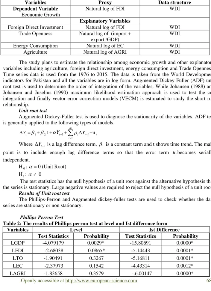
The study plans to estimate the relationship among economic growth and other explanatory variables including agriculture, foreign direct investment, energy consumption and Trade Openness. Time series data is used from the 1976 to 2015. The data is taken from the World Development indicators for Pakistan and all the variables are in log form. Augmented Dickey Fuller (ADF) unit root test is used to determine the order of integration of the variables. While Johansen (1988) and Johansen and Juselius (1990) maximum likelihood estimation approach is used to test the co- integration and finally vector error correction models (VECM) is estimated to study the short run relationship.

Unit root test

Augmented Dickey-Fuller test is used to diagnose the stationarity of the variables. ADF test is generally applied to the following types of models.

1 Y  =₁+₂t +



Y_t_₁+ _t _i m t i Y  



1  +u_t

Where Y_t__i is a lag difference term, ₁ is a constant term and t shows time trend. The main point is to include enough lag difference terms so that the error term utbecomes serially independent.

H₀: = 0 (Unit Root) H1:   0

The test statistics has the null hypothesis of a unit root against the alternative hypothesis that the series is stationary. Large negative values are required to reject the null hypothesis of a unit root.

Results of Unit root test

The Phillips-Perron and Augmented dickey-fuller tests are used to check whether the data series are stationary or non stationary.

PhillipsPerron Test

Table 2: The results of Phillips perron test at level and Ist difference form

Variables Level Ist Difference

Test Statistics Probability Test Statistics Probability

LGDP -4.079179 0.0029* -15.80691 0.0000*

LFDI -2.68038 0.0865* -5.14443 0.0001*

LTO -1.90491 0.3267 -5.16811 0.0001*

LEC -2.37973 0.1542 -4.43314 0.0012*

(5)

Interpretations

The above table shows that GDP and FDI are stationary at the significance level of 0.05% so in this case the H0 is rejected. But AGRI, EC and TO are non significant at the level. However all the variables are stationary at Ist difference 0.05% level.

Augmented Dickey – Fuller Test

Table 3: Result of Augmented Dickey Fuller test at level Ist difference form

Variables Level Ist Difference

Test Statistics Probability Test Statistics Probability

LGDP -4.07918 0.0029 * -9.32611 0.0000* LFDI -2.66819 0.0887 * -5.15009 0.0001 * LTO -1.81573 0.3676 -5.16851 0.0001 * LEC -2.550835 0.1122 -4.34444 0.0015* LAGRI -1.83586 0.3582 -6.00151 0.0000 * Interpretations

The above table shows that all the variables are stationary at Ist difference.

Figure 1 Quartile Diagram showing GDP, FDI, Trade Openness, Energy Consumption and Agriculture 0.0 0.2 0.4 0.6 0.8 1.0 1.2 0.0 0.2 0.4 0.6 0.8 1.0 1.2 Quantiles of LGDP Q u a n ti le s o f N o rm a l LGDP -1.2 -0.8 -0.4 0.0 0.4 0.8 -1.5 -1.0 -0.5 0.0 0.5 1.0 Quantiles of LFDI Q u a n ti le s o f N o rm a l LFDI 2.4 2.5 2.6 2.7 2.8 2.45 2.50 2.55 2.60 2.65 2.70 2.75 Quantiles of LEC Q u a n ti le s o f N o rm a l LEC 1.30 1.35 1.40 1.45 1.50 1.55 1.32 1.36 1.40 1.44 1.48 1.52 Quantiles of LAGRI Q u a n ti le s o f N o rm a l LAGRI -.2 .0 .2 .4 .6 .8 .0 .1 .2 .3 .4 .5 .6 .7 Quantiles of LTO Q u a n ti le s o f N o rm a l LTO

(6)

Interpretation

The output displays the perfect normal distribution, the red line, and the actual observations, the blue dots, within each group. As we can that see there exists only minor deviations from the red line, therefore we conclude that the assumption concerning normal distributed errors is satisfied.

Co-integration

The study applies co-integration test to check the long run relationship among the variables. Mainly there are two ways to test co integration.

1. The Engle – Granger two step method.

2. The Johansen and Juselius, Johansson (1998) procedure.

Engle and Granger (1987) co integration test

The Johansen co integration test is used to test the long-run movement of the variables which requires only variables with the same order of integration.

Johansen & Juselius (1990) and Johansson (1998)

Johansen co integration test is utilized to check the long-run development of the variables (Johansen 1988; Johansen 1991). In this method all variables should be integrated at same order i.e integrated at Ist difference. If the results showed that all variables are cointegrated, then we will check error correction model (ECM).

The test is taking into account the most extreme probability estimation of the K-dimensional Vector Autoregression (VAR). We use the Trace (Tr) eigenvalue measurement and Maximum (L-max) eigenvalue measurement (Johansen 1988; Johansen and Juselius 1990).

Co-integration test

Table 4: The result of Johansen co-integration test among GDP, FDI, Trade Openness, Energy Consumption, & Agriculture Rate

Panel A Trace Test

Hypothesized Trace 95%

No. of CE(s) Eigenvalue Statistic Critical Value Prob.

None * 0.981231 219.6209 69.81889 0.0000**

At most 1 * 0.729475 88.42856 47.85613 0.0000**

At most 2 * 0.463913 45.2847 29.79707 0.0004*

At most 3* 0.348427 24.71053 15.49471 0.0016* At most 4* 0.274169 10.57446 3.841466 0.0011*

Panel B Maximum Eigenvalue

Hypothesized Max-Eigen 95%

No. of CE(s) Eigenvalue Statistic Critical Value Prob.

None * 0.981231 131.1924 33.87687 0.0000**

At most 1* 0.729475 43.14387 27.58434 0.0002*

At most 2 0.463913 20.57416 21.13162 0.0597

At most 3 0.348427 14.13608 14.2646 0.0524

Panel C. Normalized cointegrating coefficients

LGDP = 0.378313LFDI + 0.967329LEC + 0.053658LAGRI + 0.107387LTO

(0.02109) (0.03883) (0.00055) (0.01903)

[17.9380]* [24.911]* [97.56]* [5.6430]* .

(7)

Openly accessible at http://www.european-science.com 692 The trace test statistically demonstrates that there are 5 cointegrating associations. There subsists an exclusive LR association among GDP, EC, TO, FDI and AGRI. An economic interpretation of the LR function can be obtained by normalizing the estimates of the unconstrained cointegrating vector on the GDP.

The outcomes in panel-C of Table-5 show an affirmative and significant association among these variables, which is consistent with economic theory ; In long run, trade openness have a major impact on the human capital and economic growth ( Aurangzeb and Malik et al. 2010). Moreover FDI has positive impact on economic growth in long run {Khan et al (2011), Aurangzaib et al (2011) and Yousaf et al. (2008)}. Energy consumption also has positive impact on economic growth both in long and short run {Masih & Masih(1996), Khan & Ahmad(2009) and Rufael(2010)}. Likewise, {Anthony (2010), Awokuse(2009) and Akram Waqar et al.(2006)} also show positive impact of agriculture on economic growth in long run, which is consistent with the current study results.

Error Correction Model

For short run analysis, the study used the Vector Error Correction Mechanism. It measures the speed of adjustment to restore equilibrium. The results of VCM show that the adjustment process is statistically significant.

Diagnostic Statistics: BG=0.81926(0.075), ARCH(1)=0.1577(0.6937),

RESET=1.261960(0.2696), JB [χ2 (2)]=0.3093(0.8567), Hetroscedasticity White=0.79985(0.6612)

Note: ARCH: Engle’s test for conditional heteroskedasticity; BG: Breusch-Godfrey LM (4) test for serial correlation; Hetroscedasticity White JB:Jarque-Bera test for normality of residuals Based on test of Skewness and Kurtosis of residuals;RESET: Ramsey’s test for specification error. [Probability values are in the squared brackets].

The consequences of VECM and many diagnosotic tests are presented in Table – 5. Due to change in results of ECM for GDP is superior significant at 1%. This involves that a Granger causality (GC) runs from AGRI, EC, FDI and TO to GDP in Pak. The outcome demonstrates that there is an affirmative effect of AGRI, EC and TO on GDP in SR. Since FDI has pessimistic impact on GDP in SR. The pessimistic sign demonstrates that the model is convergent in the direction of balance and the value shows the speed of modification of the model. It means that adjustment speed of previous year disequilibrium to current year is 8 % of FDI.

Diagnostic tests of Model

Diagnostic test is conducted to observe the issues of serial correlation and Hetroscedasticity. The value of DW-Statistics is 2.051056 therefore it is concluded that there is no problem of autocorrelation. The Diagnostic test clearly demonstrates no problem of serial correlation, Hetroscedasticity, Lagrange Multiplier (LM), Normality and Ramsey Reset Test.

The diagnostic tests reported in Table-6 show that there is no evidence of diagnostic problem with the model. Looking at the probability value of the Jarque-Bera (JB), which is given in the bracket, the null hypothesis of normally distributed residuals cannot be rejected. The Lagrange Multiplier (LM) test of no error autocorrelation suggests that the residuals are not serially correlated. The Autoregressive Conditional Heteoskedasticity test reveals that the disturbance term in the equation is homoskedastic. The Ramsey RESET test result shows that the calculated F-value is less than the critical value at the five percent level of significance. This is an indication that there is no specification error.

(8)

Table 5: Results of the Error correction model

Impulse Response Analysis

The impulse response function is presented in the following Figure Error Correction: D(LOG_GD

P)

D(LOG_FDI) D(LOG_TO) D(LOG_EC) D(LOG_AGRI)

CointEq1 Coefficient 0.115465 -0.084342 0.05226 0.000229 0.016033 Standard Error (0.07289) (0.05292) (0.02339) (0.00226) (0.00374) t-Stat [ 1.58407] [-1.59374] [2.23432] [ 0.10172] [ 4.29193] D(LOG_GDP(-1)) Coefficient -0.612821 0.351154 0.148147 0.012548 -0.026693 Standard Error (0.44373) (0.32215) (0.14238) (0.01373) (0.02274) t-Stat [-1.38108] [ 1.09002] [ 1.04047] [ 0.91368] [-1.17384] D(LOG_GDP(-2)) Coefficient -0.246977 0.238004 0.034513 0.020904 -0.00216 Standard Error (0.43638) (0.31682) (0.14003) (0.01351) (0.02236) t-Stat [-0.56596] [ 0.75122] [ 0.24647] [ 1.54769] [-0.09658] D(LOG_FDI(-1)) Coefficient -0.345103 0.084987 0.158303 -0.004835 -0.003732 Standard Error (0.31043) (0.22538) (0.09961) (0.00961) (0.01591) t-Stat [-1.11170] [ 0.37709] [ 1.58920] [-0.50324] [-0.23458] D(LOG_FDI(-2)) Coefficient -0.23678 0.015705 0.172008 0.014752 -0.013177 Standard Error (0.24796) (0.18002) (0.07957) (0.00767) (0.01271) t-Stat [-0.95490] [ 0.08724] [ 2.16181] [ 1.92216] [-1.03698] D(LOG_TO(-1)) Coefficient -1.462488 1.382758 0.444392 0.006198 -0.201734 Standard Error (1.66942) (1.21203) (0.53569) (0.05167) (0.08555) t-Stat [-0.87605] [ 1.14086] [ 0.82957] [ 0.11995] [-2.35797] D(LOG_TO(-2)) Coefficient -0.916048 1.172623 0.316424 0.045885 -0.040589 Standard Error (1.40865) (1.02271) (0.45201) (0.04360) (0.07219) t-Stat [-0.65030] [ 1.14659] [ 0.70003] [ 1.05243] [-0.56225] D(LOG_EC(-1)) Coefficient -1.225015 -1.617743 -0.243563 -0.041031 0.268072 Standard Error (7.10066) (5.15521) (2.27849) (0.21977) (0.36389) t-Stat [-0.17252] [-0.31381] [-0.10690] [-0.18670] [ 0.73668] D(LOG_EC(-2)) Coefficient -2.078863 0.002753 -1.721264 0.026783 0.951769 Standard Error (6.31694) (4.58621) (2.02700) (0.19551) (0.32373) t-Stat [-0.32909] [ 0.00060] [-0.84917] [ 0.13699] [ 2.94001] D(LOG_AGRI(-1)) Coefficient -4.256503 -3.974157 0.574333 -0.017458 -0.399284 Standard Error (3.50945) (2.54793) (1.12613) (0.10862) (0.17985) t-Stat [-1.21287] [-1.55976] [ 0.51001] [-0.16072] [-2.22007] D(LOG_AGRI(-2)) Coefficient -6.20023 0.050333 2.552346 -0.104214 -0.297207 Standard Error (3.76491) (2.73340) (1.20810) (0.11653) (0.19294) t-Stat [-1.64684] [ 0.01841] [ 2.11269] [-0.89433] [-1.54038] R-squared 0.419099 0.447929 0.536589 0.642236 0.660250 Adj. R-squared 0.102243 0.146799 0.283819 0.447092 0.474931 F-statistic 1.322681 1.487494 2.122837 3.291085 3.562787

(9)

Figure 2: Impulse Response Function

Figure 2 represents that the result of S.D of all variables. According to the results impulse responses do appear very responsive. However, results show the positive impact of other four variables on GDP.

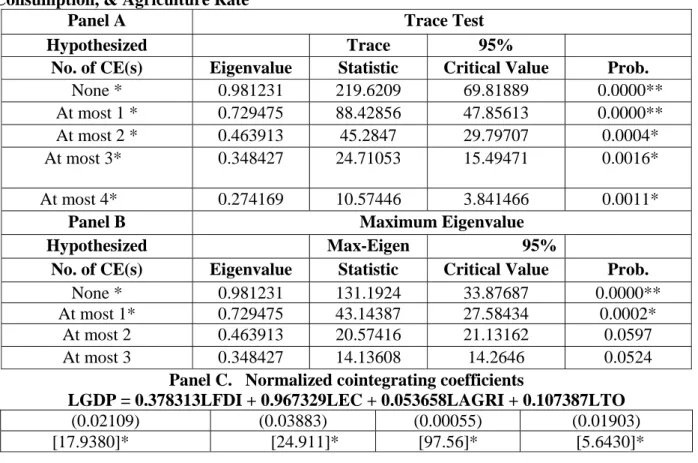
Table 6 supplied some portion of the forecast error variance for every variable that is accredited to its own development and development in the other variable. A considerable source of variation in growth forecast error with respect to the time, ranging from 100% to 65%, is represented by the shocks of real GDP (economic growth). The fluctuations in economic growth are accounted by TO (5%), AGRI (12%) and FDI (14%) shocks while that of EC (2%) is somewhat little in Pakistan after ten years. Therefore the predominant sources of variation in GDP are Agriculture and FDI. Analogous elucidations embrace for the variations in growth in the other forecast epoch. This demonstrates that the GC runs from AGRI Growth Rate, EC, TO and FDI to GDP. -0.4 -0.2 0.0 0.2 0.4 0.6 0.8 1.0 1 2 3 4 5 6 7 8 9 10 LGDP LFDI LEC LAGRI LT O

Res pons e of LGDP to Choles ky One S.D. Innovations -0.5 0.0 0.5 1.0 1.5 2.0 1 2 3 4 5 6 7 8 9 10 LGDP LFDI LEC LAGRI LT O

Res pons e of LFDI to Choles ky One S.D. Innovations -12 -8 -4 0 4 8 1 2 3 4 5 6 7 8 9 10 LGDP LFDI LEC LAGRI LT O

Res pons e of LEC to Choles ky One S.D. Innovations -0.5 0.0 0.5 1.0 1.5 2.0 1 2 3 4 5 6 7 8 9 10 LGDP LFDI LEC LAGRI LT O

Res pons e of LAGRI to Choles ky One S.D. Innovations -0.8 -0.4 0.0 0.4 0.8 1.2 1 2 3 4 5 6 7 8 9 10 LGDP LFDI LEC LAGRI LT O

Res pons e of LTO to Choles ky One S.D. Innovations

(10)

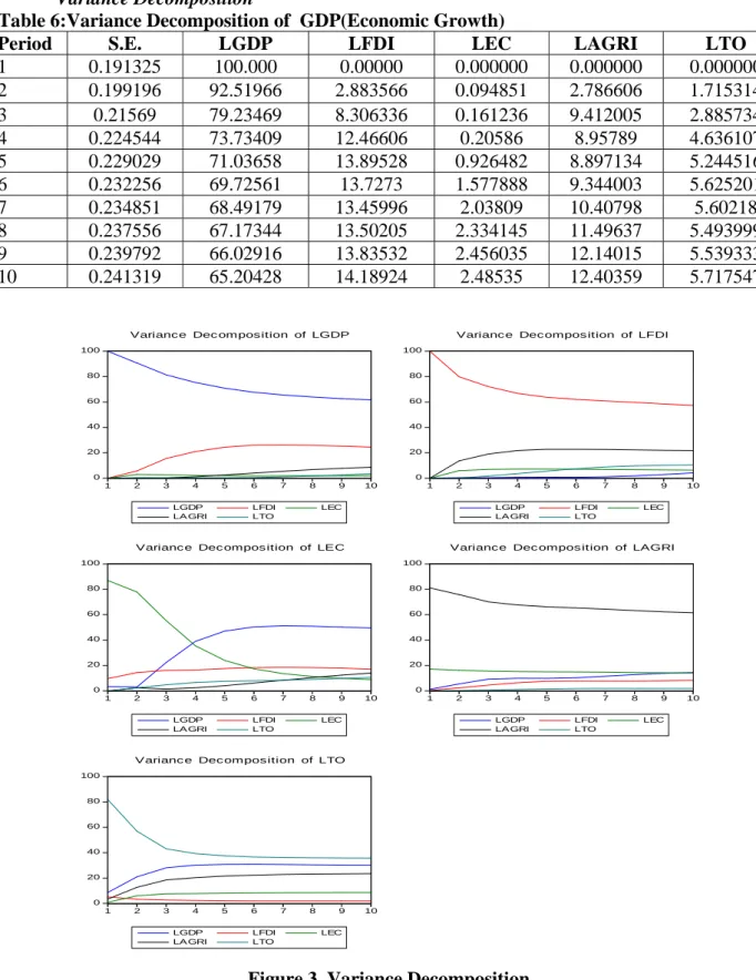
Decomposition of Variance Analysis

Variance Decomposition

Table 6:Variance Decomposition of GDP(Economic Growth)

Period S.E. LGDP LFDI LEC LAGRI LTO

1 0.191325 100.000 0.00000 0.000000 0.000000 0.000000 2 0.199196 92.51966 2.883566 0.094851 2.786606 1.715314 3 0.21569 79.23469 8.306336 0.161236 9.412005 2.885734 4 0.224544 73.73409 12.46606 0.20586 8.95789 4.636107 5 0.229029 71.03658 13.89528 0.926482 8.897134 5.244516 6 0.232256 69.72561 13.7273 1.577888 9.344003 5.625201 7 0.234851 68.49179 13.45996 2.03809 10.40798 5.60218 8 0.237556 67.17344 13.50205 2.334145 11.49637 5.493999 9 0.239792 66.02916 13.83532 2.456035 12.14015 5.539333 10 0.241319 65.20428 14.18924 2.48535 12.40359 5.717547

Figure 3. Variance Decomposition

0 20 40 60 80 100 1 2 3 4 5 6 7 8 9 10 LGDP LFDI LEC LA GRI LTO

Variance Dec omposition of LGDP

Varianc e Decompos ition of LFDI

Varianc e Dec ompos ition of LEC

Variance Dec ompos ition of LAGRI

(11)

Block Exogeneity Tests

This technique is applied to the results causality between these variables, how the data enter in the model. It is a multivariate generalization of Granger causality tests.

Table 7: VAR Granger Causality/Block Exogeneity Wald Tests Dependent variable: D(LOG_GDP)

Excluded Chi-sq Df Prob.

D(LOGFDI) 3.644816 2 0.1616

D(LOGEC) 0.041219 2 0.9796

D(LOGAGRI) 2.128978 2 0.03449

D(LOGTO) 4.976079 2 0.0831

All 10.04992 8 0.2615

The block of exogeneity tests in Table-7 reveal that AGRI growth rate and TO should enter the model at two lags. This demonstrates that the GC runs from AGRI & TO to GDP (economic growth), which opposes theory and experimental research in terms of FDI and EC, Only agriculture and TO are significant in the model.

Conclusion and Policy Recommendations

Conclusion

This study is designed to check the relationship among foreign direct investment (FDI), energy utilization (EC), Trade Openness(TO), Agriculture and monetary development (GDP) and also the effect of these variables on financial development in Pak. A causality investigation of the FDI, EC, TO, AGRI and GDP were attempted keeping in mind the end goal to check the importance of the monetary development theory in the Pak economy.

The study used technique to check the data analysis and LR Co integration relationship among agriculture, TO, EC, FDI and GDP for Pak using Johansen multivariate Co-integration technique. The basic objective of our research is to investigate the determinants of GDP. For this purpose time series data were used from 1976-2015. GDP is the dependant variable and agriculture, TO, EC, FDI, is used in the analysis as explanatory variable.

The results explained that all the four explanatory variables are significant in LR. In LR there is positive impact of agriculture, TO, EC, FDI and GDP on economic growth, although there is positive for short run as shown by VECM except foreign direct investment because FDI is negative impact on GDP for short run as shown by VECM.

The outcomes show that in case of Pakistan, agriculture, TO, EC, FDI and GDP are major determinants of GDP to country.

However, the block of Exogeneity tests shows that the Granger causality runs from agriculture, Trade Openness, Energy Consumption and Foreign direct investment on economic growth . Only agriculture and energy consumption are significant. However, the result of the error correction model shows that there is a positive, negative, positive and negative effect of agriculture, Trade Openness, Energy Consumption and Foreign direct investment on GDP respectively.

Policy Recommendations

(12)

Openly accessible at http://www.european-science.com 697  Government should focus on these policies that embark increase and diversification in

exports and decrease in imports. Local markets and infant industries should be promoted and subsidized.

 Government should concentrate more on the production of agriculture sector. Government should provide relevant information to the farmers, conduct research and must initiate workshops and training centers to educate and train them in order to advance the field of agriculture and food science and work in sectors such as production, promotion and preservation. Agricultural culture can be edified at different school levels, post school and adult levels.

 It is prescribed that the policy makers and governments should ponder on improving framework, settle political environment, and build human assets to enhance financial development of Pakistan.

 Encouraging and inviting environment should be furnished to the foreign investors in order to pull more FDI into our economy.

 Industrialization is the best way of achieving economic solidity of a country. Industrial sector of Pakistan can’t . The slow pace of industrial development is the Most of the current economic tribulations in Pakistan are eventually connected to. Rapid industrialization is considered by the economic exports as the sovereign remedy to put our economy on a sound basis. industrial sector. Harbinger creature create escort to

 Industrial sector also helps government to stabilize price in country when goods are available in sufficient quantity, there is n0 change of increasing prices of these items. A nation which depends upon the production and export of raw material alone cannot achieve a rapid rate people. Industrialization increases the income of the workers. It enhances their capacity to save. The voluntary savings stimulate industrial growth and by cumulative effect lead to further expansion of industry. A country’s industrial sector is crucial for its enhanced economic performance as it increases the per capita income and is pivotal for the economic development of a country.

 Unfortunately, the industrial sector has been either stagnating or declining in Pakistan, therefore per capita income is not growing at the desired rate. The share of industrial sector was around 25% in the GDP in early 2000 and has declined to around 20.50% which has become too low considering the level of economic development of Pakistan. There are certain factors associated with this decline.

 Speculation and remittances have played a significant role in jacking up land prices. The unplanned expansion of cities without taking into account proper zoning regulation added salt to injury. The land booms of 2002-2006 and 2011-2016 have increased their prices manifold in metropolitan cities of Pakistan.

 These skyrocketed land prices have increased the opportunity cost for setting up a factory. As a consequence, the industrialists started to seek ‘land rents’ and diverted their attention from their core business of establishing and expanding the industry.

(13)

References

Agrawal, G., Aamir Khan, M. (2011). Impact of FDI on GDP Growth: A Panel Data Study. European Journal of Scientific Research, 57(2), 257-264.

Africa: Evidence from panel data analysis. Journal of applied Economics & Finance, 3, (1), 145- 160.

Amjad, S; Hasnu & SAF. (2007). Smallholders’ Access to Rural Credit: Evidence from Pakistan. The Lahore Journal of Economics, 12 (2), 1-25.

A.Waheed & S.T. Jawaid (2006).”Inward Foreign Direct Investment and Aggregate Imports: Journal of Time Series Evidence from Pakistan, 33-43.

Authokorala, P. W. (2003). The Impact of Foreign Direct Investment for Economic Growth: a case study of Sri Lanka. International Conference for Sri Lanka Studies, 8(92),1-21.

Ahmad, N. (2013). The role of budget deficit in the economic growth of Pakistan. Global Journal of Management & Business Research, Economics & Commerce, 13, (5).

Amjad R (2010). Key Challenges Facing Pakistan Agriculture: How Best Can Policy Makers Respond? A Note. Paper presented in the GDN 11th Annual Conference held at Prague, Czech Republic. http://pide.org.pk/pdf/foodsecurity/research/FS1.pdf

Anwer, M. S. & sampath, R. K. (1999). Investment & economic growth. Western agriculture economic association. http://ageconsearch.umn.edu/bitstream/35713/1/sp99an01.pdf

Asafu-Adjaye, J. (2000). The relationship between energy consumption, energy prices and economic growth: time series evidence from Asian developing countries. Journal of energy economics, 22, 615-625.

Baffes, J. (2004). Cotton, market setting, trade policies and issues. World Bank Policy Research. Working journal ,3218, 1-76.

Bashir, Z. (2003). The impact of economic reforms and trade liberalization on agricultural export performance in Pakistan. The Pakistan Dev. Review, 42(4), 941-960.

Bayar, Y. (2016). Impact of openness and economic freedom on economic growth in the transition economies of the European Union. South eastern Europe Journal of Economics, 1, 7 -19. Bibi.S,. Ahmad, S.T. & Rashid, H. (2014). Impact of Trade Openness, FDI, Exchange Rate and

Inflation on Economic Growth: A Case Study of Pakistan. International Journal of Accounting and Financial Reporting, 4, (2), 236-257.

Chaudhry.S.I., Safdar, N. & Farooq, F. (2012). Energy Consumption and Economic Growth: Empirical Evidence from Pakistan. Pakistan Journal of Social Sciences, 32, (2), 371-382. Chowdhury, A. & Mavratos, G. (2006).FDI and growth: what causes what? The World Economy,

29(1), 9-19.

Chaitanya Vadlamannati, K. & Tamazian, A. (2010). Growth effects of foreign direct investment and economic policy reforms in Latin America. MPRA, 14133.

Cheng, B. S.& T. W. Lai (1997). An Investigation of Co-integration and Causality between Energy Consumption and Economic Activity in Taiwan. Journal of Energy Economics,19 (4), 435– 444. https://en.wikipedia.org/wiki/Economy_of_Pakistan

Gallo, C. (2002). Economic growth and income inequality: theoretical background and empiricalevidence.https://www.bartlett.ucl.ac.uk/dpu/publications/latest/publications/dpu-working-papers/WP119.pdf Gross domestic product. In Wikipedia, Retrieved September 3, 2016

Helliwell, J. Layard, R. & Sachs, J. (2012). World happiness report. http://www.earth.columbia.edu/sitefiles/file/Sachs%20Writing/2012/World%20Happiness% 20Report.pdf

(14)

Openly accessible at http://www.european-science.com 699 Hull, K. (2009). Understanding the Relationship between Economic Growth, Employment and

Poverty Reduction. http://www.oecd.org/derec/unitedkingdom/40700982.pdf

Khan, M. A. (2007). Foreign direct investment and economic growth: The role of domestic financial

sector. PIDE Working Paper. http://saber.eastasiaforum.org/testing/eaber/sites/default/files/documents/PIDE_Khan_2007_

05.pdf

Kuznets, S. (1955). Economic growth and income inequality. Journal of American Economic Review, 45, (1), 1-28.

Manggoel, W. (2012). Agriculture as a mitigating factor to unemployment in Nigeria. Journal of Agricultural Science and Soil Science, 2, (11), 465-468.

Matthew, A. & Mordecia, D.B. (2016). The impact of agricultural output on economic development in Nigeria: 1986-2014. Journal of archives of current research international, 4, (1), 1-10. Mckay, A. & Sumner, A. (2008). Economic growth, inequality & poverty reduction: Does pro-poor

growth matter? (3). https://www.ids.ac.uk/files/NewNo2-Poverty-web.pdf

Mencinger, J. (2003). Does foreign direct investment always enhance economic growth? Journal of KYKLOS, 56, (4), 491-508.

Musila, J.W. & Yiheyis, Z. (2015). The impact of trade openness on growth: The case of Kenya. Journal of policy modeling, 37, 342-354.

Mallick, H. (2009). Examining the linkage between energy consumption and economic growth in India, The Journal of Developing Areas, 4(3), 249-280

Menegaki, A. N. (2011). Growth and renewable energy in Europe a random effect model with evidence for neutrality hypothesis, Energy Economics, 3(3), 257-263.

McKinnon, R.I. (1990). ”Financial Depression and the Productivity of Capital: Empirical Findings on Interest Rates and Exchange Rates” 1(1), 1-15

Raza, S. A., Yasir, A. & Mehboob, F. (2012). Role of agriculture in economic growth of Pakistan. Journal of finance & economics, (83), 181-186.

Roemer, M. & Gugerty, M. K. (1997). Does Economic Growth Reduce Poverty? Consulting Assistance on Economic Reform.http://pdf.usaid.gov/pdf_docs/Pnaca656.pdf

Roubini, N. & Sachs, J. D. (1989). Political and economic determinants of budget deficits in the industrial democracies. Journal of European Economic review, 33, 903-938.

Sama, M. C. & Tah, N.R. (2016). The effect of energy consumption on economic growth in Cameroon. Journal of Asian economic and financial review, 6(9), 510-521.

Siddiqui, R. (2004). Energy and economic growth in Pakistan. Journal of Pakistan development review, 43,(2), 175-200.

Sharmiladevi, J. C. (2016). A review of the effects of foreign direct investment on economic growth. Journal of Symbiosis center for management studies, 4,126-131.

Subramaniam V, & Reed, M. (2009). Agricultural Inter-Sectoral Linkages and its Contribution to Economics Growth in the Transition Countries, the International Association of Agricultural

Economists Conference, Beijing, China.

http://ageconsearch.umn.edu/bitstream/51586/2/438a.pdf

Wang, M., & Wong, M. C. S. (2009). Foreign Direct Investment and Economic Growth: The Growth Accounting Perspective. Journal of Economic Inquiry, 47(4): 701-710.

World Development Indicators (2010). World Bank, Washington DC. @ http://data .worldbank.org/ data-catalog/world-development-indicators.

Yu, S. H. & J. Y. Choi, (1985). “The Causal Relationship between Energy and GNP: An International Comparison”. Journal of Energy and Development, 11 (2 ), 249-272.

(15)

Openly accessible at http://www.european-science.com 700 Yang, H. Y. (2000). A Note on the Causal Relationship between Energy and GDP inTaiwan. Journal

of Energy Economics, 22(3), 309–317.

Zekarias, S.M.(2016). The impact of foreign direct investment on economic growth in eastern Africa: Evidence from panel data analysis. Journal of applied Economics & Finance, 3, (1), 145-160.

Zuberi HA (1989). Production Function, Institutional Credit and Agricultural Development in Pakistan. The Pakistan Development Reveiew, 28( 1), 35-45.

Zhang, Y-J. (2011). Interpreting the Dynamic Nexus between Energy Consumption and Economic Growth: Empirical Evidence from Russia. Journal of Energy Policy, 39, 2265-2272.

Zeb.N, Qiang. F, & Rauf .S (2013). Role of Foreign Direct Investment in Economic Growth of Pakistan ,International Journal of Economics and Finance; 6 (1), 1916-9728.