Use of soft computing and numerical analysis in design, analysis and management of pavement systems

(1)

2019

Use of soft computing and numerical analysis in

design, analysis and management of pavement

systems

Orhan Kaya Iowa State University

Follow this and additional works at:https://lib.dr.iastate.edu/etd Part of theCivil Engineering Commons

This Dissertation is brought to you for free and open access by the Iowa State University Capstones, Theses and Dissertations at Iowa State University Digital Repository. It has been accepted for inclusion in Graduate Theses and Dissertations by an authorized administrator of Iowa State University Digital Repository. For more information, please [email protected].

Recommended Citation

Kaya, Orhan, "Use of soft computing and numerical analysis in design, analysis and management of pavement systems" (2019).

Graduate Theses and Dissertations. 17035. https://lib.dr.iastate.edu/etd/17035

(2)

by

Orhan Kaya

A dissertation submitted to the graduate faculty

in partial fulfillment of the requirements for the degree of

DOCTOR OF PHILOSOPHY

Major: Civil Engineering (Transportation Engineering; Civil Engineering Materials)

Program of Study Committee: Halil Ceylan, Major Professor

Jing Dong Sunghwan Kim Omar G. Smadi Paul G. Spry Peter C. Taylor

The student author, whose presentation of the scholarship herein was approved by the program of study committee, is solely responsible for the content of this dissertation. The

Graduate College will ensure this dissertation is globally accessible and will not permit alterations after a degree is conferred.

Iowa State University

Ames, Iowa

2019

(3)

DEDICATION

(4)

TABLE OF CONTENTS

Page

LIST OF FIGURES ... vi

LIST OF TABLES ... xii

ACKNOWLEDGMENTS ... xiii

ABSTRACT ... xiv

CHAPTER 1. GENERAL INTRODUCTION ... 1

Motivation ... 4

Objectives ... 5

Dissertation Organization ... 6

References ... 8

CHAPTER 2. NEURAL-NETWORK BASED MULTIPLE-SLAB RESPONSE MODELS FOR TOP-DOWN CRACKING MODE IN AIRFIELD PAVEMENT DESIGN ... 10

Abstract ... 10

Introduction ... 11

Synthetic Database Development ... 14

ANN Model Development ... 19

Mechanical-Load-Only Case ... 19

Use of individual input parameters (approach 1) ... 19

Use of dimensional analysis (approach 2) ... 23

Simultaneous Mechanical and Thermal Loading Case ... 29

Use of individual input parameters (approach 1) ... 29

Use of dimensional analysis (approach 2) ... 30

Summary, Conclusions and Future Work ... 34

Acknowledgements ... 36

References ... 36

CHAPTER 3. NUMERICAL ANALYSIS OF LONGITUDINAL CRACKING IN WIDENED JOINTED PLAIN CONCRETE PAVEMENT SYSTEMS ... 39

Abstract ... 39

Introduction ... 40

Numerical Modeling Approach ... 42

Single Axle Load Simulations ... 44

Single Axle Load Simulation Results ... 46

Truck Load Simulations ... 49

Three-Axle Truck with 6.1 m (20 ft.) Axle Spacing Placed on a Single Slab ... 50

Four-Axle Truck with 7.0 m (23 ft.) Axle Spacing with both Axle Groups Partially Placed on Adjacent Slabs ... 54

(5)

Shoulder Design Alternatives Simulations ... 59

Tied PCC Shoulder ... 62

HMA Shoulder ... 62

Shoulder Design Alternatives Simulations - Summary of Findings ... 66

Conclusions, Discussions, and Recommendations ... 66

References ... 70

CHAPTER 4. EVALUATION OF RIGID AIRFIELD PAVEMENT CRACKING FAILURE MODELS ... 71

Abstract ... 71

Introduction ... 72

Objectives ... 72

Review of Current FAARFIELD Rigid Airfield Pavement Design Methodology ... 73

Inclusion of Top-down and Bottom-up Failure Modes in Rigid Airfield Pavement Design ... 78

Stress Comparisons ... 79

Design Slab Thickness Calculations ... 89

Conclusions ... 94

Recommendations ... 97

References ... 98

CHAPTER 5. DEVELOPMENT OF A FRAMEWORK FOR PROJECT AND NETWORK LEVEL PAVEMENT PERFORMANCE AND REMAINING SERVICE LIFE PREDICTION MODELS FOR IOWA PAVEMENT SYSTEMS ... 100

Abstract ... 100

Introduction ... 101

Objectives ... 102

Descriptions of Overall Approaches and Data Preparation ... 103

Project Level Pavement Performance Model Development and Accuracy Evaluations ... 109

Project Level Pavement RSL Model Development and Results ... 112

Network Level Pavement Performance Model Development and Accuracy Evaluations ... 118

JPCP Pavement Performance Models for Network Level ... 120

Flexible Pavement Performance Models for Network Level ... 125

Composite (AC over JPCP) Pavement Performance Models for Network Level ... 132

Network-Level Pavement RSL Model Development and Results ... 139

JPCP RSL Models for Network Level ... 140

Flexible Pavement RSL Models for Network Level ... 145

Composite (AC over JPCP) Pavement RSL Models for Network Level ... 149

Discussion: Comparisons between Statistical and AI based Network Level Pavement Performance Models ... 153

(6)

JPCP Pavement Case ... 154

Flexible Pavement Case ... 155

Composite (AC over JPCP) Pavement Case ... 156

Conclusions and Recommendations ... 157

Overall Conclusions ... 157

Conclusions for JPCP ... 160

Conclusions for Flexible Pavements ... 161

Conclusions for Composite (AC over JPCP) Pavements ... 162

References ... 164

CHAPTER 6. CONCLUSIONS, RECOMMENDATIONS AND CONTRIBUTIONS OF THIS STUDY TO THE LITERATURE AND TO THE PAVEMENT ENGINEERING FIELD ... 167

Conclusions ... 167

Contributions of this Study to the Literature and to the Pavement Engineering Field ... 177

(7)

LIST OF FIGURES

Page

Figure 1.1 A data-driven and efficient pavement design, analysis and management

concept ... 5

Figure 1.2 Modeling methods used in this study ... 6

Figure 2.1 Accuracy improvement using different number of cases in the

development of ANN models in terms of (a) R2_{and (b) MSE ... 17}

Figure 2.2 Aircraft loading conditions ... 18

Figure 2.3 Twelve individual input parameters used in the development of ANN

models (mechanical-load-only case) ... 20

Figure 2.4 ANN network architecture (individual input parameters,

mechanical-load-only case) ... 21

Figure 2.5 Accuracy comparison using different number of hidden neurons in the

development of ANN models in terms of (a) R2_{and (b) MSE ... 22}

Figure 2.6 FEAFAA solutions vs. ANN predictions for (a) σxx, max, top-tensile; (b) σyy,

max, top-tensile; (c) τxy, max, top; (d) δmax (individual input parameters,

Figure 2.7 ANN network architecture (dimensional analysis, mechanical-load-only case) ... 28

max, top-tensile; (c) τxy, max, top; (d) δmax (dimensional analysis,

Figure 2.9 Fourteen types of individual input parameters (simultaneous mechanical and thermal loading case) ... 30

max, top-tensile; (c) τxy, max, top; (d) δmax (individual input parameters,

simultaneous mechanical and thermal load case) ... 31

max, top-tensile; (c) τxy, max, top; (d) δmax (dimensional analysis, simultaneous mechanical and thermal load case) ... 33

(8)

Figure 3.1 FEA model definitions ... 42

Figure 3.2 Single-axle load cases ... 45

Figure 3.3 Top and bottom tensile stress ratio distribution for single axle mechanical load combined with three different temperature load scenarios; (a) ΔT=

0 ◦C (0 ◦F), (b) - 5.5 ◦C (-10 ◦F), and (c) ΔT= -11◦C (-20 ◦F) applied on

various locations in both traffic and wander directions. ... 47

Figure 3.4 Top-to-bottom tensile stress ratio distribution for various combined

mechanical and temperature load cases ... 49

Figure 3.5 Failure mechanism for longitudinal cracking from field investigation ... 50

Figure 3.6 Three-axle truck with 6.1 m. (20 ft.) axle spacing – discretized truck load .... 51

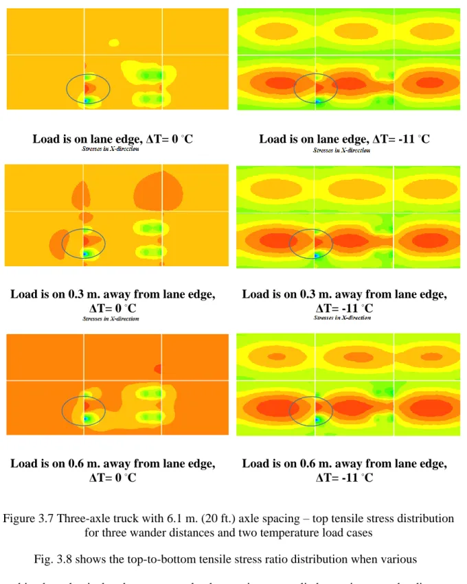
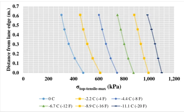
Figure 3.7 Three-axle truck with 6.1 m. (20 ft.) axle spacing – top tensile stress

distribution for three wander distances and two temperature load cases ... 52

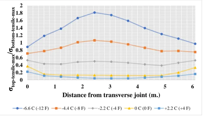
Figure 3.8 Three-axle truck with 6.1 m. (20 ft.) axle spacing – top-to-bottom tensile stress ratio distribution ... 53

Figure 3.9 Three-axle truck with 6.1 m. (20 ft.) axle spacing – top tensile stress

distribution ... 54

Figure 3.10 Top tensile stress transfer mechanism in four-axle truck ... 55

Figure 3.11 Four-axle truck – discretized truck load ... 56

Figure 3.12 Four-axle truck – top tensile stress distribution for four temperature load cases ... 56

Figure 3.13 Four-axle truck – top-to-bottom tensile stress ratio distribution ... 57

Figure 3.14 Four-axle truck – top tensile stress distribution ... 58

Figure 3.15 Comparisons of tensile stress distributions between a three-axle truck

and a four-axle truck ... 58

Figure 3.16 Shoulder design alternatives ... 60

Figure 3.17 Widened and regular size slabs with shoulder design alternatives ... 61

Figure 3.18 Top-to-bottom tensile stress ratio and top tensile stress comparisons between a widened slab with partial-depth tied PCC shoulder and a

(9)

Figure 3.19 Comparisons of tensile stress distributions between widened and regular slabs with an HMA shoulder ... 64

Figure 3.20 Top-to-bottom tensile stress ratio comparisons between widened slab with an HMA shoulder, regular slab an HMA shoulder and regular slab with a full-depth tied PCC shoulder ... 65

Figure 4.1 Slab thickness determination in FAARFIELD ... 74

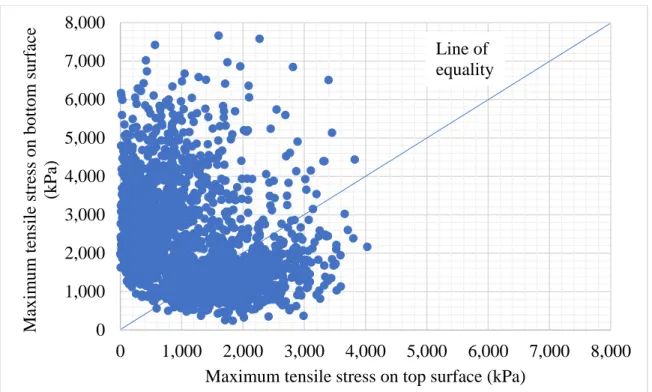
Figure 4.2 Maximum (a) tensile and (b) principal stress distribution at the bottom

and top slab surfaces for 2,000 cases ... 83

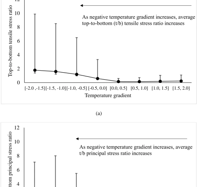
Figure 4.3 Top-to-bottom (a) tensile and (b) principal stress ratio distribution for

2,000 cases ... 85

Figure 4.4 Top-to-bottom (a) tensile and (b) principal stress ratio distribution for

various temperature gradient cases ... 86

Figure 4.5 Distribution of applied mechanical load... 87

Figure 4.6 Distribution of critical pavement response locations where maximum top (a) tensile and (b) principal stresses were observed ... 88

Figure 4.7 Mechanical load locations: (a) corner load and (b) edge load ... 90

Figure 5.1 Pavement performance and RSL model development stages ... 104

Figure 5.2 Comparisons between before and after data preparation methodology was applied in a flexible pavement section based on three pavement

performance indicators: a) IRI, b) longitudinal cracking and c)

transverse cracking (US 18, MP 212.74 to 214.39, E, Traffic (AADTT): 1,885, Construction year: 2000) ... 108

Figure 5.3 IRI prediction model results and equations for a new JPCP, new flexible and composite (AC over JPCP) pavement sections as examples ... 110

Figure 5.4 Project level “tunable” pavement performance prediction automation tool . 112 Figure 5.5 IRI model changes as more data points are added into the model

development dataset as an example for a flexible pavement section (IA 3, MP 039.09 to 044.12, E, Traffic (AADTT): 500, Construction year: 1999) ... 113

(10)

Figure 5.7 RSL distribution for JPCP pavement sections (a) based on pavement

section ID and (b) based on pavement length ... 115

Figure 5.8 RSL distribution for flexible pavement sections (a) based on pavement

section ID and (b) based on pavement length ... 116

Figure 5.9 RSL distribution for composite (AC over JPCP) pavement sections (a)

based on pavement section ID and (b) based on pavement length ... 117

Figure 5.10 Network level pavement performance prediction automation tool ... 119

Figure 5.11 Comparisons between measured pavement condition records and ANN model predictions using a) transverse cracking, b) IRI (approach 1) and c) IRI (approach 2) ANN models for JPCP pavements ... 121

Figure 5.12 Comparisons between measured pavement condition records and ANN model predictions using a) transverse cracking, b) IRI (approach 1) and c) IRI (approach 2) ANN models, respectively, for a JPCP pavement section as an example (IA 5, MP 85.24 to 88.06, N, Traffic (AADTT): 799, Construction year: 1999) ... 123

Figure 5.13 Comparisons between measured pavement condition records and ANN

model predictions usinga) rutting, b) longitudinal cracking, c)

transverse cracking, d) IRI (approach 1) and e) IRI (approach 2) ANN models for flexible pavements ... 127

Figure 5.14 Comparisons between measured pavement condition records and ANN model predictions using a) rutting, b) longitudinal cracking, c)

transverse cracking, d) IRI (approach 1) and e) IRI (approach 2) ANN models, respectively, for a flexible pavement section as an example (US 18, MP 212.74 to 214.39, E, Traffic (AADTT): 1,885,

Construction year: 2000) ... 129

transverse cracking, d) IRI (approach 1) and e) IRI (approach 2) ANN models for composite pavements ... 134

transverse cracking, d) IRI (approach 1) and e) IRI (approach 2) ANN models, respectively, for a composite pavement section as an example (US 20, MP 1.64 to 4.37, E, Traffic (AADTT): 2,848, Restoration year: 2004) ... 136

(11)

Figure 5.17 Network level RSL calculation steps ... 140

Figure 5.18 RSL distribution for JPCP pavement sections(a) based on pavement

section ID and (b) based on pavement length, when transverse cracking model and percent cracking threshold limit of 15% were used ... 141

Figure 5.19 RSL distribution for JPCP pavement sections (a) based on pavement section ID and (b) based on pavement length, when IRI (approach 1)

model and threshold limit of 170 in/mile were used ... 143

Figure 5.20 RSL distribution for JPCP pavement sections (a) based on pavement section ID and (b) based on pavement length, when IRI (approach 2)

Figure 5.21 RSL distribution for flexible pavement sections(a) based on pavement

section ID and (b) based on pavement length, when rutting model and threshold limit of 0.4 in. were used ... 146

Figure 5.22 RSL distribution for flexible pavement sections(a) based on pavement

section ID and (b) based on pavement length, when IRI (approach 1)

Figure 5.23 RSL distribution for flexible pavement sections (a) based on pavement section ID and (b) based on pavement length, when IRI (approach 2)

Figure 5.24 RSL distribution for composite pavement sections (a) based on pavement section ID and (b) based on pavement length, when rutting

model and threshold limit of 0.4 in. were used ... 150

Figure 5.25 RSL distribution for composite pavement sections (a) based on pavement section ID and (b) based on pavement length, when IRI

model (approach 1) and threshold limit of 170 in/mile were used ... 151

Figure 5.26 RSL distribution for composite pavement sections (a) based on pavement section ID and (b) based on pavement length, when IRI

model (approach 2) and threshold limit of 170 in/mile were used ... 152

Figure 5.27 Accuracy comparisons between statistical and ANN based network

level IRI models for JPCP pavements ... 155

(12)

(13)

LIST OF TABLES

Page

Table 2.1 Ranges of inputs used for FEAFAA batch runs ... 18

Table 2.2 Accuracy comparison of the ANN models in predicting pavement

responses for different cases ... 34

Table 3.1 FEA model inputs ... 43

Table 4.1 Types and ranges of input parameters used in FEAFAA runs ... 80

Table 4.2 Types of input parameters used in FEAFAA runs for thickness

calculations ... 89

Table 4.3 Slab Thickness comparisons using FAARFIELD Version 1.42 design

methodology ... 93

Table 4.4 Summary of slab thickness comparisons ... 94

Table 5.1 Pavement condition rating thresholds determined by FHWA (10) ... 106

Table 5.2 Summary of input and output parameters used in three ANN Models

development for JPCP pavements ... 121

Table 5.3 Summary of input and output parameters used in five ANN models

development for flexible pavements ... 126

Table 5.4 Summary of Input and output parameters used in five ANN models

(14)

ACKNOWLEDGMENTS

First of all, I would like to thank my major professor, Dr. Halil Ceylan, for his

support in this study. I especially admire his technical knowledge, academic dedication

and multitasking.

Furthermore, I would like to thank my committee members, Drs. Sunghwan Kim,

Jing Dong, Peter C. Taylor, Omar G. Smadi and Paul G. Spry for their guidance and

support throughout the course of this research. Special thanks are extended to Dr.

Sunghwan Kim who inspired me with his diligence with respect to work discipline,

academic dedication and patience.

In addition, I would like to thank the Ministry of National Education of Turkey

for providing me with a scholarship and educational opportunity in the U.S.

Last but not least, I would like to thank my beloved parents, Mustafa and Fatma,

and siblings, Osman, Okan and Handan, for their endless love and support throughout my

(15)

ABSTRACT

There are a number of components of pavement engineering, including pavement

management, pavement analysis and design, and pavement materials. Historically, the

field of pavement management has been interested in monitoring post-construction

condition, timing of preventive maintenance and rehabilitation treatments, and economic

analysis of alternatives. On the other hand, the field of pavement analysis and design has

dealt with optimizing pavement structure; with optimum structure, a pavement system is

expected to survive during its service life for given traffic and climate conditions. The

performance of pavement materials has been improved to achieve the long-lasting and

lower-maintenance pavement systems. A data-driven comprehensive approach

considering all aspects of pavement engineering together could be a future direction for

advancing pavement engineering practices.

In order to achieve a data-driven comprehensive approach considering all aspects

of pavement engineering together as outlined above, a data-driven and efficient pavement

design, analysis and management concept has been proposed in this study. To serve as

elements of this concept, several models related to pavement structural response models,

pavement performance prediction models, and pavement remaining service life (RSL)

models have been developed. First, to enable faster three-dimensional finite element

(3D-FE) computations of design stresses, artificial neural network (ANN)-based surrogate

computational pavement structural response models were developed. These models

produce an estimate of the top-down bending stress close to that computed by 3D-FE

analysis in rigid airport pavements in a fraction of the time. Second, longitudinal cracking

(16)

their longitudinal cracking potential was evaluated using numerical analysis. Third, the

Federal Aviation Administration’s (FAA) current rigid airfield pavement design

methodology has been evaluated in great detail to better identify research gaps and

remaining needs with respect to cracking failure models so that recommendations could

be made as to how current methodology could be improved to accommodate top-down

and bottom-up cracking failure modes. Fourth, a detailed step-by-step methodology for

the development of a framework for pavement performance and RSL prediction models

was explained using real pavement performance data obtained from the Iowa Department

(17)

CHAPTER 1. GENERAL INTRODUCTION

Pavements are designed to withstand several types of loads, including traffic and

environmental loads, and pavements develop structural responses such as stresses, strains,

and deflections when they are exposed to such loads. Structural-response models have been

developed to estimate structural response of pavements to various load types and magnitudes.

State-of-the-art practice in pavement response modeling is to use mechanistic-based models.

Mechanistic-empirical pavement design guide (AASHTOWare Pavement ME Design

computer program) uses finite-element analysis (FEA) based pavement response models for

rigid pavement design and analysis, while it uses two approaches (two-dimensional nonlinear

finite-element analysis for the most general case of nonlinear unbound material behavior and

multilayer elastic theory (MLET) for the case of purely linear material behavior) for flexible

pavement design and analysis (NCHRP 2003). Similarly, with the arrival of New Large

Aircraft (NLA) and associated design challenges for pavement designers, including

increasing airplane weights and complex gear configurations, the Federal Aviation

Administration (FAA) has adopted layered elastic theory for flexible airport pavement design

and three-dimensional finite-element (3D-FE) procedures for rigid airport pavement design

(FAA 2014). In summary, numerical analysis techniques such as finite-element models

comprise state-of-the-art practice for rigid pavement structural response modeling and, along

with LEA, they also represent state-of-the art practices for flexible pavement structural

response modeling.

Pavement performance models are used to evaluate how pavement performance

changes over time. Pavement performance models can be categorized into two groups,

(18)

Sundin and Braban-Lexdoux 2001; Albuquerque and Broten 1997). Deterministic models

estimate single condition values at a given time in the design life of pavements, while

probabilistic models estimate the probability of each condition value at a given time (Chen

and Mastin 2016). Most state highway agencies (SHAs) use deterministic models as part of

their pavement management systems for various reasons, including (1) ease of explanation of

models to users and (2) ease of incorporating models into their pavement management

systems (PMS) (Wolters and Zimmerman 2010).

Mechanistic-empirical pavement design guide (AASHTOWare Pavement ME Design

computer program) follows mechanistic-empirical pavement design methodology in which

empirical transfer functions relate pavement structural responses to pavement performance

estimations (NCHRP 2003). FAA’s pavement thickness design computer program FAA Rigid and Flexible Iterative Elastic Layer Design (FAARFIELD) also follows a

mechanistic-empirical design methodology in its pavement design computations (FAA 2014).

SHAs are required to develop performance-based approaches in their pavement

management decision-making processes based on the Moving Ahead for Progress in the 21st

Century (MAP-21) Federal Transportation Legislation (HR 2012). One performance-based

approach to facilitating the pavement management decision-making process is to use

remaining service life (RSL) models. RSL for pavements can be defined as the time frame

between the present time and the time when a significant rehabilitation treatment or

reconstruction should occur (FHWA 2018). Although application of a structural overlay or

reconstruction would normally be regarded as a sign for termination of pavement service life,

(19)

(FHWA 2018). RSL models, developed to predict the remaining life of pavements, are being

used as elements of the pavement management process. (Elkins et al. 2013).

Multiple advantages of RSL have been reported in the literature (Mack and Sullivan

2014) and its key positive features include:

 Estimation of the time, expressed in years, before rehabilitation would be required for

any given road section

 Ease of understanding (especially for public)

 Can be a multi-conditional measure developed from any type of functional and/or

structural data

 Allowing agencies to distinguish between two road sections with the same current

condition (i.e., the same current International roughness index (IRI))

 Providing deeper insight by converting “condition measures” into an “operational

performance” measure that tells how well or how long the road will continue serving the public

 Providing an ideal tool for addressing the transportation planning and performance

management criteria requirements of MAP-21 legislation

Soft computing techniques such as artificial neural networks (ANNs) have been used

to model complex pavement engineering problems (Kaya et al. 2017, Kaya et al. 2018).

ANN-based models are very effective tools for modeling pavement response and

performance, complex problems where various inputs are involved, and by providing

complex relationships between inputs and outputs. They have great potential for producing

accurate stress predictions in a fraction of the time required by traditional FE-based design

(20)

computation times. They can also easily and quickly produce pavement performance

predictions, especially in network level analysis where thousands of pavement scenarios with

various traffic loads, thicknesses, and conditions can be analyzed in seconds.

Motivation

There are a number of components of pavement engineering, including pavement

management, pavement analysis and design, and pavement materials. Historically, the field

of pavement management has been interested in monitoring post-construction condition,

timing of preventive maintenance and rehabilitation treatments, and economic analysis of

alternatives. On the other hand, the field of pavement analysis and design has dealt with

optimizing pavement structure; with optimum structure, a pavement system is expected to

survive during its service life for given traffic and climate conditions. The performance of

pavement materials has been improved to achieve the long-lasting and lower-maintenance

pavement systems. A data-driven comprehensive approach considering all aspects of

pavement engineering together could be a future direction for advancing pavement

engineering practices. In such an approach: (1) mechanisms between various pavement

materials and structures must be well-understood and well-modeled, (2) for given pavement

structures under various traffic and climate conditions, pavement performance must be

well-evaluated, (3) remaining service lives based on pavement performance model results must be

well-estimated, and (4) to optimize RSL, various pavement preservation or rehabilitation

techniques should be considered during the pavement design process. If such a data-driven

comprehensive approach could be achieved, pavement structures would be better-optimized

and designed during the design stage, potentially avoiding excessive costs because of

overdesign or early failure of pavements. Such a system could be efficient, interrelated,

(21)

Objectives

To achieve a data-driven comprehensive approach that considers all aspects of

pavement engineering together, as outlined above, this study proposes the data-driven and

efficient pavement design, analysis, and management concept portrayed in Figure 1.1. In this

concept, pavement structural response models relate structural, traffic and climatic inputs to

pavement responses, and the pavement responses are related to pavement performance

indicators using pavement performance-prediction models. Finally, pavement

remaining-service-life models are used to relate pavement performance predictions to remaining service

life estimations.

Figure 1.1 A data-driven and efficient pavement design, analysis and management concept

Figure 1.2 shows modeling methods that have been used in the development of

models described in Figure 1.1. As part of this study, the following methods have been used

in development of pavement structural response models, pavement performance prediction

models, and pavement remaining-service-life models: soft computing and numerical analysis

Source: Bolling (2012) Pavement Structural Response Models Pavement Performance Prediction Models Pavement Remaining Service Life Models

(22)

methods were used in the development of pavement structural response models; soft

computing and statistical methods were used in the development of pavement

performance-prediction models, and soft computing and statistical methods were used in the development

of pavement remaining-service-life models.

Figure 1.2 Modeling methods used in this study

Dissertation Organization

This dissertation consists of six chapters:

Chapter 1 provides some background about this study, including its motivation and

objectives.

Chapter 2 discusses development of ANN-based surrogate computational response

models or procedures (suitable for implementation in FAARFIELD 2.0, a research version of

the FAARFIELD computer program) that return close estimates of top-down bending

stresses in rigid airport pavements normally computed through 3D-FE analysis. The

Soft Computing and Numerical Analysis Soft Computing and Statistical Methods

Soft Computing and Statistical Methods

Source: ky.acpa.org

(23)

developed ANN-based surrogate computational response models enable faster 3D-FE

computations of design stresses in FAARFIELD 2.0, making it suitable for routine design.

Chapter 3 demonstrates longitudinal cracking mechanisms of widened jointed plain

concrete pavements (JPCP) and evaluates their longitudinal cracking potential using

numerical analysis. The critical load configuration with the highest longitudinal cracking

potential for widened JPCP is identified. Three different shoulder design alternatives are also

compared in terms of their contribution to mitigation of longitudinal cracking potential.

Chapter 4 evaluates FAA's current rigid airfield pavement design methodology in

great detail to better identify research gaps and needs with respect to cracking-failure models,

and provides recommendations for how current methodology could be improved to

accommodate both top-down and bottom-up cracking failure modes.

Chapter 5 describes a detailed step-by-step methodology for development of a

framework for pavement performance, and RSL prediction models using real pavement

performance data obtained from the Iowa DOT PMIS database. To develop RSL models,

project and network level pavement performance models are initially developed using two

approaches: a statistically (or mathematically) defined approach for project-level model

development, and an artificial intelligence (AI) based approach for network-level model

development. Using pavement performance models for various pavement performance

indicators (IRI for project level models, and rutting, percent cracking, and IRI for network

level models) and the Federal Highway Agency (FHWA)-specified threshold limits for these

pavement performance indicators, RSL models are then developed for three pavement types:

flexible pavements, JPCP, and composite (Asphalt concrete (AC) over JPCP) pavements.

(24)

Chapter 6 describes and summarizes conclusions, recommendations, and

contributions of this study to the literature of the pavement-engineering field.

The research work described in Chapters 2 through 5 can be used as part of the

proposed data-driven and efficient pavement design, analysis, and management concept.

References

Albuquerque, N. M., and Broten, M. (1997). “Local agency pavement management

application guide.” Project 1-37A, Washington State Dept. of Transportation, Olympia, WA. Bolling, D. (2012). “Pavement preservation: Getting ahead of the curve for locals”.

Proceedings of the 37th Annual Rocky Mountain Asphalt Conference and Equipment.

Chen, D. and Mastin N. (2016). “Sigmoidal models for predicting pavement performance conditions. ASCE J. Perform. Constr. Facil., 2016, 30(4): 04015078.

FAA. (2014). “Airport design”. FAA Advisory Circular (AC) No: 150/5300-13A.

FHWA. (2018). “Pavement health track remaining service life (RSL) forecasting models, Technical Information”.

G. E. Elkins, T. M. Thompson, J. L., Groeger, B. Visintine, and G. R. Rada. (2013). “Reformulated pavement remaining service life framework”. FHWA.

HR. (2012). “Moving ahead for progress in the 21st_{century act (MAP–21)”. An Act}

to authorize funds for Federal-aid highways, highway safety programs, and transit programs, and for other purposes, 112 Congress, 2nd Session. Enacted October 1, 2012.

Kaya, O., A. Rezaei-Tarahomi, H. Ceylan, K. Gopalakrishnan, S. Kim, and D.R. Brill. (2018). “Neural network–based multiple-slab response models for top-down cracking mode in airfield pavement design”. Journal of Transportation Engineering, Part B: Pavements, 2018. 144 (2).

Kaya, O., A. Rezaei-Tarahomi, H. Ceylan, K. Gopalakrishnan, S. Kim, and D.R. Brill. (2017). “Developing rigid airport pavement multiple-slab response models for top-down cracking mode using artificial neural networks”. Presented at 2017 TRB Annual Meeting, Washington D.C.

Mack, J. W. and Sullivan, R. L. (2014). “Using remaining service life as the national

performance measure of pavement assets”. Proceedings of the 93rd_{Annual Meeting of the}

(25)

NCHRP (2003). “Guide for mechanistic-empirical design of new and rehabilitated pavement structures”. Champaign, IL.

Sundin, S., and Braban-Lexdoux, C. (2001). “Artificial intelligence-based decision support technologies in pavement management.” Comput. Aided Civ. Infrastruct. Eng., 16(2), 143– 157.

Wolters, A. S., and Zimmerman, K. A. (2010). “Current practices in pavement performance modeling, project 08-03 (C07), task 4 report: Final summary of findings.” Penn DOT, Harrisburg, PA.

(26)

CHAPTER 2. NEURAL-NETWORK BASED MULTIPLE-SLAB RESPONSE MODELS FOR TOP-DOWN CRACKING MODE IN AIRFIELD PAVEMENT

DESIGN

A journal paper published in Journal of Transportation Engineering: Part B, Pavements

Orhan Kaya, Adel Rezaei-Tarahomi, Halil Ceylan, Kasthurirangan Gopalakrishnan,

Sunghwan Kim and David R. Brill

Abstract

The Federal Aviation Administration (FAA) has recognized for some time that its

current rigid pavement design model, involving a single slab loaded at one edge by a single

aircraft gear, is inadequate with respect to top-down cracking. Thus, one of the major

observed failure modes for rigid pavements is poorly accounted for in the FAA Rigid and

Flexible Iterative Elastic Layer Design (FAARFIELD) design software. A research version

of the FAARFIELD design software (Version 2.0) has been developed, in which the

single-slab three-dimensional finite element (FE) response model is replaced by a four-single-slab

3D-FE model with initial temperature curling to produce reasonable thickness designs

accounting for top-down cracking behavior. However, the long and unpredictable run times

associated with the four-slab model and curled slabs make routine design with this model

impractical. Artificial intelligence (AI) based alternatives such as artificial neural networks

(ANNs) have great potential to produce accurate stress predictions in a fraction of the time.

ANNs could be practical replacements for a full 3D-FE computation that requires long

computation times. In the development of ANN models, both individual input parameters and

dimensional analysis have been considered and accuracy of predictions from both methods

was compared. ANN models for only mechanical and simultaneous mechanical and thermal

(27)

was observed that very high accuracies were achieved in predicting pavement responses for

all cases investigated.

Introduction

Airport pavements are designed to withstand repeated loading imposed by aircraft, to

resist detrimental effects of traffic, and to endure deterioration induced by adverse weather

conditions (e.g., extreme hot or cold weather) and other influences. A typical civil airport is

serviced by a fleet of aircraft with different weights and gear configurations and the airport

pavement is thus designed to withstand the repeated traffic loading of the entire range of

aircraft, not just the heaviest aircraft (FAA 2014), over many years. Historical airport

pavement design methodologies were based on simplified formulas (California Bearing Ratio

(CBR) and Westergaard equations) combined with observations of field performance. With

the arrival of New Large Aircraft (NLA) and the associated design challenges for pavements,

including increasing airplane weights and complex gear configurations, the FAA adopted

layered elastic theory for flexible airport pavement design and three-dimensional finite

element (3D-FE) procedures for rigid airport pavement design. These mechanistic-empirical

design methodologies, implemented in the FAA Rigid and Flexible Iterative Elastic Layer

Design (FAARFIELD) design software (Version 1.41), are robust and can be adapted for

addressing future gear configurations without modifying the underlying procedures (FAA

2014).

For rigid pavement design, FAARFIELDuses a 3D-FE computer program called

NIKE3D_FAA to compute the maximum horizontal stress at the bottom edge of the Portland

Cement Concrete (PCC) slab as the pavement structural life predictor. NIKE3D_FAA is a

modification of the NIKE3D program originally developed by the Lawrence Livermore

(28)

limiting horizontal stress at the bottom of the PCC slab, cracking of the surface layer, (the

only rigid pavement failure mode considered by FAARFIELD), is controlled. FAARFIELD

currently does not consider the failure of subbase and subgrade layers. For a given airplane

traffic mix over a particular subgrade/subbase, FAARFIELDprovides the required rigid

pavement slab thickness (FAA 2009).

The FAA has also developed FEAFAA (Finite Element Analysis – FAA), which

makes use of NIKE3D, as a stand-alone tool for 3D-FE analysis of multiple-slab rigid airport

pavements and overlays. It computes accurate responses (deflections, stresses and strains) of

rigid pavements to individual aircraft landing gear loads. FEAFAA is a research and analysis

tool; however, it is not a full-pledged design tool as it lacks the empirical components of

FAARFIELD. At the same time, FEAFAA allows more options and greater configurability

than the standard 3D-FE mesh implemented in FAARFIELD.

The FAA’s current rigid pavement design model, involving a single slab loaded at one edge by a single aircraft gear, is inadequate to account for top-down cracking. Thus, one

of the major observed failure modes for rigid pavements is poorly accounted for in the

FAARFIELD rigid design procedure. To account for the influence of top-down cracking in

thickness design, research version of the FAARFIELD design software has been developed,

in which the single-slab three-dimensional finite element (3D-FE) response model is replaced

by a four-slab 3D-FE model with initial temperature curling and variable joint spacing

(FAARFIELD Version 2.0). However, the long and unpredictable run times associated with

the four-slab model and curled slabs make routine design with this model impractical. To

expand the FAARFIELD design model beyond the current one-slab model, the FAA is

(29)

Artificial intelligence (AI) based alternatives such as artificial neural networks (ANNs) have

great potential to produce accurate stress predictions in a fraction of the time of traditional

FE-based design programs. ANNs could be practical alternatives to replace a full 3D-FE

computation that requires long computation times.

The capability of ANN-based surrogate response models to successfully compute all

components of tensile stresses as well as deflections at the bottom of jointed concrete airfield

pavements has already been illustrated by many studies (Ceylan et al. 1999; Ceylan 2002;

Rezaei-Tarahomi et al. 2017a). Some of the input parameters used in these response models

were function of type, level, and location of the applied gear load, slab thickness, slab

modulus, subgrade support, pavement temperature gradient, and the load transfer efficiencies

of the joints.

The objective of this paper is to develop ANN-based surrogate computational

response models or procedures (suitable for implementation in FAARFIELD (Version 2.0))

that return a close estimate of the top-down bending stress computed by NIKE3D in rigid

airport pavements. This will enable faster 3D-FE computations of design stresses in

FAARFIELD (Version 2.0) making it suitable for routine design. To develop these ANN

models, the authors used FEAFAA, the FAA software for stand-alone 3D-FE rigid pavement

stress computations. A synthetic database consisting of FEAFAA input parameters and the

associated critical pavement responses were created to develop ANN-based surrogate

computational response models. This database was developed using the following automated

process:

 Step 1: Generate several cases with randomly generated FEAFAA input parameters

(30)

 Step 2: Run FEAFAA one case at a time

 Step 3: Extract critical pavement responses from FEAFAA output file

 Step 4: Enter the extracted critical pavement responses into the database

 Step 5: Repeat steps 2-4 for all the cases generated in step 1

In the FEAFAA batch runs, two different load cases were considered and ANN

models were developed for these two cases: Case 1: mechanical-load-only, and Case 2:

simultaneous mechanical and temperature loading. During the ANN model development for

each loading case, two approaches were followed:

 Approach 1: Use all individual input parameters as independent inputs in the

development of ANN models

 Approach 2: Use dimensional analysis to reduce the number of inputs in the development

of ANN models

The feasibility of dimensional analysis in the ANN model development for the

top-down cracking mode was also investigated. The purpose was to evaluate whether ANN

models with acceptable prediction accuracies can be obtained with a reduced number of input

parameters (Langhaar 1951; Taylor 1974). Dimensional analysis has been successfully used

in the past in developing pavement response prediction models (Ceylan 2002; Khazanovich

et al. 2001; Ioannides 2005; NCHRP 2003), making it a promising approach.

Synthetic Database Development

To develop an extensive database of input-output records from FEAFAA 2.0, a tool

was developed by using the C# programming language together with the AutoIt®_scripting

tool (Autoit 2017) that minimizes the required time to supply the software with inputs and to

(31)

automatically perform batch runs, obtain the outputs, and then perform the post processing.

The post-processing can extract the critical pavement responses along with critical pavement

response locations. For each FEAFAA run, critical pavement responses on the top surface of

the PCC slab were specified and collected.

A preliminary analysis was carried out to determine the minimum number of samples

(i.e., FEAFAA batch runs) to ensure the robustness of the ANN models and to eliminate any

possible errors associated with sampling. A set of batch runs were executed for ANN model

development using the six-wheel Boeing B777-300ER mechanical-load-only case, σxx, max,

top-tensile (individual input parameters, mechanical-load-only case), which will be discussed later

in this paper. The preliminary analysis used groups of 100, 250, 500 and 939 normally

distributed random sampling numbers within the predefined range. Ten consecutive ANN

models were developed for each group (100, 250, 500 and 939) to quantify the variance

between each ANN model developed, if any. That is, a total of 40 ANN models were

developed for this preliminary analysis. Rezaei-Tarahomi et al. (2017b) also evaluated

sensitivity of critical pavement responses to each input variation.

The accuracy of ANN models was quantified by statistical indices R2_{(Coefficient of}

determination) and MSE (Mean squared error) as defined in Equations (2.1) and (2.2). In

addition, the standard deviations of statistical indices for ten consecutive ANN models per

each group were calculated and presented as error bar along with average of each statistical

index in Fig. 2.1. 𝑅2 = (1 𝑛× ∑ [(𝑦_𝑗𝑠𝑜𝑙𝑢𝑡𝑖𝑜𝑛−𝑦_{𝑚𝑒𝑎𝑛}𝑠𝑜𝑙𝑢𝑡𝑖𝑜𝑛)×(𝑦_𝑗𝑝𝑟𝑒𝑑𝑖𝑐𝑡𝑖𝑜𝑛−𝑦_{𝑚𝑒𝑎𝑛}𝑝𝑟𝑒𝑑𝑖𝑐𝑡𝑖𝑜𝑛)] 𝜎_{𝑠𝑜𝑙𝑢𝑡𝑖𝑜𝑛}×𝜎_{𝑝𝑟𝑒𝑑𝑖𝑐𝑡𝑖𝑜𝑛} 𝑛 𝑗=1 ) 2 (2.1) 𝑀𝑆𝐸 = 1 𝑛× ∑ (𝑦𝑗 𝑝𝑟𝑒𝑑𝑖𝑐𝑡𝑖𝑜𝑛 − 𝑦_𝑗𝑠𝑜𝑙𝑢𝑡𝑖𝑜𝑛)2 𝑛 𝑗=1 (2.2)

(32)

Where,

ysolution ₌_{Critical pavement response from FEAFAA}

yprediction ₌_{Same critical pavement response predicted by ANN models}

σsolution = Variance of critical pavement response from FEAFAA

σprediction = Variance of same critical pavement response predicted by ANN models

Fig. 2.1 shows the accuracy improvement as the number of samples increases in

terms of mean and standard deviation of R2 and MSE. The mean R2 increases and the

average value of MSE decreases as the number of samples increases. In particular, the

variance (standard deviation) of R2 and MSE within each group decreases as the number of

samples increases.

These results indicate that the accuracy of the ANN models increase with the number

of samples. Above 500 samples, the accuracy improvement curve started to level off. A

model using 500 samples provided comparable accuracy to a model using nearly double the

number of samples. Based on this result, the authors decided to use 500 samples for each

variable for further development of the ANN models.

Table 2.1 displays the FEAFAA input parameters and their ranges used for the batch

runs. Input parameters with only one value indicate those parameters not varied. A Boeing

B777-300ER, with a gross weight of 777,000 lbs., was used as the representative aircraft for

all cases. Because of symmetry of the problem, only one of the two main aircraft gears was

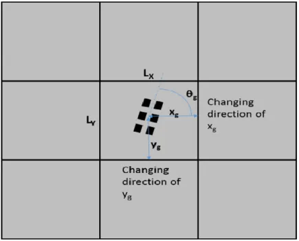
analyzed. Nine slabs with varying slab dimensions (Lx, and Ly), loading angle (θg) and gear

(33)

(a)

(b)

Figure 2.1 Accuracy improvement using different number of cases in the development of

(34)

Figure 2.2 Aircraft loading conditions

Table 2.1 Ranges of inputs used for FEAFAA batch runs

Inputs Range

Min Max

PCC Slab

Modulus GPa (psi) 20.7 (3×106₎ _{48.3 (7×10}6₎

Thickness cm. (in.) 25.4 (10) 61 (24)

Poisson Ratio 0.15 0.20

Granular Subbase

Modulus GPa (psi) 0.1 (15,000) 0.3 (50,000)

Thickness cm. (in.) 51 (20) 127 (50)

Poisson Ratio 0.35

Subgrade Modulus GPa (psi) 0.02 (3,000) (0.21) 30,000

Poisson Ratio 0.4

Slab Dimension m. (ft.) 6.1 (20) 9.1 (30)

Slab Number of Elements 30

Number of Slabs 9

Foundation Number of Elements 30

Loading Angle (deg.) 0 90

Temperature Gradient oC/cm. (oF/in.) 2.3

Thermal Coefficient 1/o_{C (1/}o_F) 7.4×10-6

(4.1×10-6)

12.9×10-6

(7.2×10-6)

(35)

ANN Model Development

ANN models were developed for both mechanical-load-only and simultaneous

mechanical and thermal load cases. For each case, both ‘approach 1’ and ‘approach 2’ were followed in the model development. In the ANN model development, a two-layer

feed-forward network was trained using a Levenberg-Marquardt algorithm (LMA) in the

MATLAB environment (MATLAB 2017).

Mechanical-Load-Only Case

The authors executed a batch run of 439 cases of B777-300ER gear loading (no

thermal load), from which they obtained the critical pavement responses required for

development of ANN models. The input variables defining the batch run set, with their

ranges, are given in Table 2.1.

Use of individual input parameters (approach 1)

As shown in Fig. 2.3, twelve input variables were used in the ANN model

development. Among these 12 input parameters, three represent the slab properties, three

represent pavement foundation properties, three represent loading location, two represent

slab size, and equivalent joint stiffness represents the joint stiffness properties of the

pavement system.

For the top-down cracking mode, stresses and deflections at the top of the slab

surface are of great interest, so critical pavement stresses and deflections at the top of the slab

surface were extracted for each case and used as outputs in the ANN model development.

The critical pavement responses used as individual outputs in the ANN model development

are as follows:

 σxx, max, top-tensile

(36)

 τxy,max, top

 δ max

Where,

σxx, max, top-tensile = Maximum tensile stress in the x direction on top of the slab surface σyy,max, top-tensile = Maximum tensile stress in the y direction on top of the slab surface τxy,max, top = Maximum shear stress on top of the slab surface

δ max = Maximum deflection

Figure 2.3 Twelve individual input parameters used in the development of ANN models (mechanical-load-only case)

Fig. 2.4 shows the ANN network architecture employed in the model development.

The ANN network consists of twelve inputs, one hidden layer with 40 hidden neurons, and

one output layer. A separate ANN model was developed to predict each pavement response.

Therefore, one output layer showing the related pavement response to be predicted and the

(37)

Figure 2.4 ANN network architecture (individual input parameters, mechanical-load-only case)

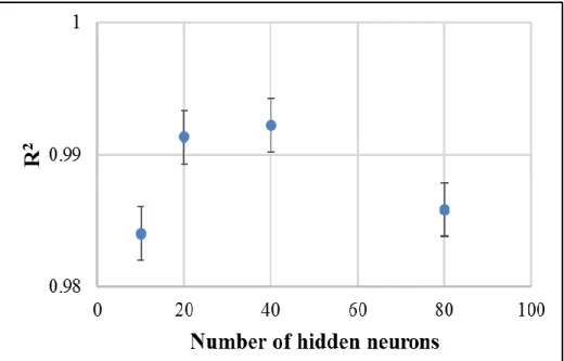
The choice of forty hidden neurons used in the hidden layer of the ANN network

architecture was made as a result of a sensitivity analysis conducted for that study. Using 500

samples for all input variables, ANN models were developed using 10, 20, 40 and 80 hidden

neurons. Fig. 2.5 shows the accuracy comparison of ANN models using different numbers of

hidden neurons. To eliminate any sampling problems, ten consecutive ANN models were

developed for each hidden neuron case. The variation in each case was quantified by the

standard deviation (Fig. 2.5). It was determined that 40 hidden neurons produced the highest

(38)

(a)

(b)

Figure 2.5 Accuracy comparison using different number of hidden neurons in the

development of ANN models in terms of (a) R2_{and (b) MSE}

Fig. 2.6 shows pavement response comparisons between the FEAFAA solutions and

(39)

For all pavement response types, in the ANN model development, 307, 66 and 66 cases were

used for training, testing and validation, respectively. For all pavement response types, ANN

models successfully replicated FEAFAA pavement response solutions. Validation and test

sets produced high accuracies comparable to the training set in all pavement response types.

This demonstrates the ANN models’ success in generalization (i.e., they did not memorize

the relationship) and so they are robust and valid.

(a) (b)

(c) (d)

Figure 2.6 FEAFAA solutions vs. ANN predictions for (a) σxx, max, top-tensile; (b) σyy, max,

top-tensile; (c) τxy, max, top; (d) δmax (individual input parameters, mechanical-load-only case)

Use of dimensional analysis (approach 2)

As mentioned previously, dimensional analysis has been used successfully in

(40)

Ioannides 2005; NCHRP 2003). Dimensional analysis has been evaluated in some FE based

pavement design and analysis applications such as ISLAB 2000 (Khazanovich 2001).

However, FEAFAA has certain unique features that no other available FE based pavement

design and analysis applications have. Among these are the use of “infinite” elements to

represent subgrades of infinite depth and a unidirectional spring element used for modeling

linear elastic joints between adjacent slabs. FEAFAA includes horizontal interfaces in its

three-dimensional model that meet the requirements of a full unbonded interface between the

slab and base course and a full bond at all other horizontal interfaces (Brill 1998). Most of

the available FE based applications have used the simplified Winkler foundation concept to

characterize the subgrade and the load transfer efficiency (LTE) concept for joints. These

unique features needed to be incorporated in the dimensional analysis.

In FEAFAA, an equivalent shear stiffness kjoint, characterizes the joint, in units of

force per relative vertical displacement per unit length of the joint. Joints were modeled in

such a way that they act as linear elastic springs between adjacent slabs, transmitting vertical

loads between adjacent slabs in shear through the joint. The shear force is assumed linearly

proportional to the relative vertical displacement between slabs (Hooke’s law) (Brill 1998).

A value for kjoint can be either input to FEAFAA directly or the software can calculate a value

from dowel bar diameter, dowel bar spacing and joint opening information. The range of

values for kjoint used in this study is shown in Table 2.1. In some previous studies, joints have

been characterized by the LTE concept and a dimensionless parameter of AGG/kl (explained

later in this paper) was used to represent joint behavior of the pavement (Ceylan 2002;

Ioannides 2005). However, for FEAFAA, kjoint has to be used in joint characterization and a

(41)

In FEAFAA, subgrade is modeled as an elastic solid; therefore, it is characterized by

elastic properties: the elastic modulus (Esubgrade) and Poisson’s ratio. In addition, the subgrade

is assumed to have infinite thickness.

Dimensionless parameters identified in the previous studies were analyzed to find out

whether they can also be used in this study. The dimensionless parameters identified in the

previous studies (Ceylan 2002; Ioannides 2005; NCHRP 2003) were as follows:

 AGG/kl,  xg/Lx,  yg/Ly,  a/l,  Lx/l,  Ly/l,  l Where,

AGG = Aggregate interlock factor

k = Modulus of subgrade reaction

l = Radius of relative stiffness of the slab-subgrade system

xg = x-coordinate of applied gear load

yg = y-coordinate of applied gear load

Lx and Ly = Length and width of the slab

a = Radius of the applied load

Analyzing the parameters above, it was determined that AGG had to be replaced with

(42)

characterization of the subgrade. Since k cannot be used and k is included in radius of

relative stiffness (l) equation (Equation 2.3), this equation should be revised for this study.

Original ‘l’ equation is shown as lks, where ks stands for k value of the subgrade (s):

𝑙𝑘𝑠 = √ 𝐸 ℎ3 12 (1−𝜇2_{) 𝑘} 4 (2.3) Where, h = Slab thickness E = Modulus of elasticity of PCC

µ = Poisson's ratio for PCC

Based on the previous studies and considering the input parameters used in FEAFAA, the following parameters were determined to be used in dimensional analysis.

• kjoint h_eff/E_subgrade l,

• x_g/L_x, • y_g/L_y, • a/l, • L_x/l, • L_y/l Where,

heff = Effective thickness of two

heff equation used (Khazanovich et al. 2001),

ℎ_𝑒𝑓𝑓 = √ℎ_𝑃𝐶𝐶3 ₊𝐸𝐵𝐴𝑆𝐸 𝐸𝑃𝐶𝐶 ℎ𝐵𝐴𝑆𝐸 3 3 (2.4) Where, hPCC =Slab thickness

(43)

hBASE =Base thickness

EPCC = Modulus of elasticity of PCC

EBASE = Modulus of elasticity of base

Original l equation (Equation 2.3) was revised to make all of the parameters

dimensionless by taking into account the physical meaning of the original equation. The

revised ‘l’ equation is shown in Equation 2.5 as ‘lEs’, where E stands for Esubgradeand

subgrade (s), respectively. Note that only difference between lEs and lks is that k and h in the

lks equation were replaced by Esubgradeand heff.

‘l’ equation used in dimensional analysis: 𝑙𝐸𝑠=√

𝐸 ℎ_𝑒𝑓𝑓3

12 (1−𝜇2_{) 𝐸}_{𝑠𝑢𝑏𝑔𝑟𝑎𝑑𝑒}

3

(2.5)

The critical dimensionless pavement responses used as outputs in the ANN model development are as follows:

 σxx, max, top-tensile × h2/P

 σyy,max, top-tensile × h2/P

 τxy,max, top × h2/P

 δ max × Esubgrade × 𝑙_𝐸𝑠 2 /P Where,

h = Slab thickness

P = Applied load (a combined weight on 6 wheels in one leg of the main gear of Boeing

B777-300ER)

Fig. 2.7 shows the ANN network architecture employed in the model development if

dimensional analysis is used in the model development. As can be seen in the figure, the

(44)

output layer. The main benefit of using dimensional analysis is that the ANN model is

developed with far fewer input parameters: only six input parameters are needed in

dimensional analysis (approach 2), compared to fourteen parameters when using individual

input parameters (approach 1). Using fewer input parameters can save considerable

computational time and other resources.

Figure 2.7 ANN network architecture (dimensional analysis, mechanical-load-only case)

ANN predictions for (a) σxx, max, top-tensile,(b)σyy, max, top-tensile, (c) τxy,max, top and (d) δmax,if

dimensional analysis is used in the model development. For all pavement response types, in

the ANN model development, 307, 66 and 66 cases were used for training, testing and

validation, respectively. For all pavement response types, ANN models successfully

(45)

Simultaneous Mechanical and Thermal Loading Case

The authors executed a batch run of 500 cases of combined mechanical and thermal

loading, from which they obtained the critical pavement responses required for development

of ANN models. The input variables defining the batch run set, with their ranges, are given in

Table 2.1.

(a) (b)

(c) (d)

top-tensile; (c) τxy, max, top; (d) δmax (dimensional analysis, mechanical-load-only case)

Use of individual input parameters (approach 1)

In this approach, all individual varied input parameters were used in ANN models as

input parameters. Fig. 2.9 shows the 14 input parameters that must be used in the ANN

(46)

mechanical and thermal load case and the mechanical-load-only case is the inclusion of two

variables to simulate thermal loading. The two additional variables are shown in Fig. 2.9 as

slab temperature properties.

Figure 2.9 Fourteen types of individual input parameters (simultaneous mechanical and thermal loading case)

The ANN network architecture consisted of 14 inputs, one hidden layer with 40

hidden neurons, and one output layer.

ANN predictions for (a) σxx, max, top-tensile,(b)σyy, max, top-tensile, (c) τxy,max, top and (d) δmax. For all

response types, 350, 75 and 75 cases were used for training, testing and validation,

respectively. Similar to the previous findings, for all pavement response types, ANN models

successfully reproduced FEAFAA solutions.

Use of dimensional analysis (approach 2)

The authors executed the feasibility of using dimensional analysis in the ANN model

development for the combined mechanical and thermal load case. The only difference

compared to the mechanical- load-only case is the inclusion of dimensionless parameter to

(47)

Korenev’s original dimensionless temperature gradient (Equation 2.6) has been successfully used to represent thermal loading (Khazanovich 2001).

𝛷 =2𝛼(1+𝜇)𝑙2 ℎ2 𝑘 𝛾𝛥T (2.6) (a) (b) (c) (d)

top-tensile; (c) τxy, max, top; (d) δmax (individual input parameters, simultaneous mechanical and thermal load case)

Equation 2.6 was revised to be applicable to FEAFAA as follows:

𝛷_𝑚 = 2𝛼(1+𝜇)𝑙𝑚2

ℎ2

𝐸𝑠𝑢𝑏

(48)

Where,

α = Coefficient of thermal expansion

ΔT = Temperature difference through the slab thickness γ = Unit self-weight of PCC slab

h = Slab thickness

l= Radius of relative stiffness of the plate-subgrade system

μ = Plate Poisson’s ratio

k = Modulus of subgrade reaction

Esub = Subgrade elastic modulus

Including the dimensionless thermal gradient obtained through Equation 2.7 and other

parameters used for mechanical-load-only case, seven dimensionless parameters were

determined to be used as inputs in the ANN model development:

• kjoint/Esubgrade l, • xg/Lx, • yg/Ly, • a/l, • Lx/l, • Ly/l, • Φm

In that case, as the ANN network architecture, sixteen inputs, one hidden layer with

40 hidden neurons along with one output layer was used.

(49)

dimensional analysis is used in the model development. For all pavement response types, in

the ANN model development, 350, 75 and 75 cases were used for training, testing and

validation, respectively. Similar to previous findings, ANN models successfully reproduced

FEAFAA solutions for all pavement responses.

(a) (b)

(c) (d)

top-tensile; (c) τxy, max, top; (d) δmax (dimensional analysis, simultaneous mechanical and thermal load case)

Table 2.2 compares accuracy of the ANN models for predicting pavement responses.

Accuracy is expressed by the statistics R2 and MSE. All ANN models successfully predicted

pavement responses for both mechanical-load-only and combined mechanical and thermal

(50)

predicted pavement responses as accurately as those developed using individual input

parameters.

Table 2.2 Accuracy comparison of the ANN models in predicting pavement responses for different cases

Summary, Conclusions and Future Work

The FAA is seeking practical alternatives to running the 3D-FEM stress computation

that can reduce the time to give accurate stress predictions. Artificial intelligence (AI) based

alternatives such as artificial neural networks (ANNs) have great potential and have been

successfully used in pavement engineering to solve similar problems for decades.

This paper investigated the feasibility of developing ANN-based surrogate

computational response models or procedures (suitable for implementation in FAARFIELD

(Version 2.0)) that returns a close estimate of the top-down bending stress computed by

NIKE3D in rigid airport pavements. These models would enable faster 3D-FE computations

of design stresses in FAARFIELD (Version 2.0) making it suitable for routine design. To

develop these ANN models, FEAFAA, the FAA’s computer program for stand-alone 3D-FEM analysis of multi-slab rigid pavements, was used.

Loading Case Method

Accuracy - 𝑹𝟐 (𝑴𝑺𝑬)

σ

xx,max,

top-tensile

σ

yy,max,

top-tensile

τ

xy,max, top δmax

Mechanical-load- only case

Individual input parameters 0.995 (141) 0.980 (303) 0.995 (211) 0.998 (7.4x10-8₎ Dimensional analysis 0.996 (2.2×10-8₎ 0.996 (1.6×10-4₎ 0.998/ (1.6×10-4₎ 0.999 (8.7×10-3₎ Simultaneous mechanical and temperature load case Individual input parameters 0.996 (3,268) 0.994 (3,104) 0.994 (644) 0.997 (4.9×10-4) Dimensional analysis 0.999 (1.4×10-3) 0.999 (1.8×10-3) 0.999 (2.5×10-4) 0.999 (53)

(51)

To develop ANN-based surrogate computational response models, a synthetic

database consisting of FEAFAA input parameters and the associated critical pavement

responses was created. In the FEAFAA batch runs, two different loading cases were

considered and ANN models for these two cases were developed: mechanical-load-only and

simultaneous mechanical and temperature loading. During the ANN model development for

each loading case, two approaches were followed:

 Use all individual input parameters as independent inputs in the development of ANN

models (approach 1)

 Use dimensional analysis to reduce the number of inputs in the development of ANN

models (approach 2)

Specific conclusions of this paper are listed below:

 ANN was found to be a promising alternative in returning very close estimates of the

top-down bending stress computed by NIKE3D in rigid airport pavements. By using the

ANN models, very accurate stress predictions can be produced in a fraction of time

compared to the significant amount of time needed to perform a 3D-FE computation. For

instance, stress predictions for thousands of cases can be predicted in seconds using ANN

models compared to days, if not months, using 3D-FE computation.

 Dimensional analysis was found to be a promising method to reduce the input feature

space in ANN model development. It produced accuracies similar to those produced

using individual input parameters in the model development (see Table 2.2).

 An advantage of using dimensional analysis in the development of ANN models is that it

significantly reduces the number of required input parameters. For example, six

(52)

pavement responses, compared to fourteen individual input parameters needed for

mechanical-load-only case.

 Another advantage of using dimensional analysis in the development of ANN models is

that the use of these models can be extended for any types of pavements with the same

pavement layer configurations and the next generation aircraft with the same gear

configurations, if applicable. As long as the dimensionless parameters for the pavements

and the next generation aircraft cases are within the ranges that the ANN models were

developed, the models can be directly used for these pavements and aircraft without any

modification.

 Future studies will focus on creating ANN models for other airplane types.

Acknowledgements

The authors gratefully acknowledge the Federal Aviation Administration (FAA) for

supporting this study. The contents of this paper reflect the views of the authors who are

responsible for the facts and accuracy of the data presented within. The contents do not

necessarily reflect the official views and policies of the FAA and Iowa State University. This

paper does not constitute a standard, specification, or regulation.

References

Autoit (2017). <https://www.autoitscript.com/site/autoit/> (Aug. 1, 2017).

Brill, D. R. (1998). Development of advanced computational models for airport pavement

design. FAA Report DOT/FAA/AR-97/47. Federal Aviation Administration (FAA), Washington, D.C., Available at: http://www.tc.faa.gov/its/worldpac/techrpt/ar97-47.pdf (accessed on May 18, 2015).

Brill, D. R. (2000). Field verification of a 3D finite element rigid airport pavement model.

FAA Report DOT/FAA/AR-00/33. Federal Aviation Administration (FAA), Washington, D.C.