Hash code learning for large scale similarity search

c

HASH CODE LEARNING FOR LARGE SCALE SIMILARITY SEARCH

BY

FUREN ZHUANG

THESIS

Submitted in partial fulfillment of the requirements

for the degree of Master of Science in Electrical and Computer Engineering in the Graduate College of the

University of Illinois at Urbana-Champaign, 2019

Urbana, Illinois Adviser:

ABSTRACT

In this thesis we explore methods which learn compact hash coding schemes to encode image databases such that relevant images can be quickly retrieved when a query image is presented. We here present three contributions.

Firstly, we improve upon the bit allocation strategy of Signal-to-Noise Ra-tio MaximizaRa-tion Hashing (SMH) to produce longer hash codes without a deterioration in retrieval performance as measured by mean average preci-sion (MAP). The proposed bit allocation strategy seamlessly converts the Hamming distance between hash codes into a likelihood ratio test statistic, which is the optimal decision rule to decide if samples are related. We show via experiments that at the same false positive rate, the proposed method could obtain false negative error rates which are significantly lower than the original SMH bit allocation strategy.

Our second contribution is the extension of SMH to use a deep linear discriminant analysis (LDA) framework. The original SMH method uses features from convolutional neural networks (CNNs) trained on categorical-cross-entropy (CCE) loss, which does not explicitly impose linear separability on the latent space representation learned by the CNN. The Deep LDA frame-work allows us to obtain a non-linear transformation on the input images to obtain transformed features which are more discriminatory (samples of the same class are close together while samples of different classes are far apart) and better fit the linear Gaussian model assumed in SMH. We show that the enhanced SMH method using Deep LDA outperforms recent state-of-the-art hashing methods on single-label datasets CIFAR10 and MNIST.

Our final contribution is an unsupervised graph construction method which binarizes CNN features and allows the use of quick Hamming distance calcu-lations to approximate pairwise similarity. This graph can be used in various unsupervised hashing methods which require a similarity matrix. Current un-supervised image graph construction methods are dominated by those which

utilize the manifold structure of images in the feature space. These methods face the dilemma of needing a large dense set of data points to capture the manifold structure, but at the same time are unable to scale up to the req-uisite sample sizes due to their very high complexity. We depart from the manifold paradigm and propose an alteration relying on matching, exploiting the feature detecting capabilities of rectified linear unit (ReLU) activations to generate binary features which are robust to dataset sparsity and have significant advantages in computational runtime and storage. We show on six benchmark datasets that our proposed binary features outperform the original ones.

Furthermore we explain why the proposed binarization based on Hamming metric outperformed the original Euclidean metric. Particularly, in low-SNR regimes, such as that of features obtained from CNNs trained on another dataset, dissimilar samples have been shown to be much better separated in the Hamming metric than the Euclidean metric.

ACKNOWLEDGMENTS

I thank my advisor Professor Pierre Moulin for his continued guidance and support. I am grateful for his patience and understanding in helping me overcome the numerous difficulties I encountered in the course of my graduate studies. I particularly appreciate his rigorous approach to science which I aspire to emulate and live up to.

I thank the Agency for Science, Technology and Research, Singapore, for funding of my research. I thank Professor Reginald Tan, Ms Phebe Lim, and Ms Jamie Tan for their unwavering support during my difficult times. I thank my mentors Drs. Dim Lee Kwong, Julie Ang, Vijay Chandrasekhar, Chuan Sheng Foo, Jie Lin and Wang Zhe for helpful discussions.

In addition, I thank fellow research colleagues Amish Goel and Patrick Johnstone for friendship and camaraderie.

TABLE OF CONTENTS

LIST OF ABBREVIATIONS . . . viii

CHAPTER 1 INTRODUCTION . . . 1

CHAPTER 2 BACKGROUND . . . 3

2.1 Inverted File Index . . . 3

2.2 Retrieval Using Hash Tables . . . 4

2.3 Retrieval Using Hamming Distance . . . 5

CHAPTER 3 SIGNAL-TO-NOISE RATIO MAXIMIZATION HASH-ING AND AN IMPROVED BIT ALLOCATION STRATEGY . . . 7

3.1 SNR Maximization Hashing . . . 7

3.2 Discussion . . . 8

3.3 An Improvement on SMH . . . 9

3.4 Experimental Results . . . 11

CHAPTER 4 SNR MAXIMIZATION HASHING USING DEEP LDA 16 4.1 Deep Variational and Structural Hashing . . . 16

4.2 Supervised Semantics-preserving Deep Hashing . . . 16

4.3 SMH Using Deep LDA . . . 17

4.4 Discussion . . . 18

4.5 Experimental Results . . . 19

CHAPTER 5 UNSUPERVISED GRAPH CONSTRUCTION . . . 22

5.1 Notation . . . 22 5.2 Edge Learning . . . 22 5.3 Weight Learning . . . 23 5.4 Image Matching . . . 24 5.5 Proposed Method . . . 25 5.6 Evaluation Metrics . . . 27 5.7 Experiments . . . 28 5.8 Discussion . . . 29

CHAPTER 6 FUTURE WORK AND DISCUSSION . . . 32

6.1 Extension of SMH to Multilabel Datasets . . . 32

6.2 Uunsupervised Learning Evaluation . . . 32

6.3 Microscopic Structure . . . 34

CHAPTER 7 CONCLUSION . . . 35

LIST OF ABBREVIATIONS

ANN Approximate Nearest Neighbors CBIR Content-based Image Retrieval CCE Categorical Cross-Entropy CNN Convolutional Neural Network

DVStH Deep Variational and Structural Hashing ENN Exact Nearest Neighbors

HE Hamming Embedding

LDA Linear Discriminant Analysis

LHS Left-Hand Side

LRT Likelihood Ratio Test MAP Mean Average Precision

PCA Principal Components Analysis ReLU Rectified Linear Unit

ROC Receiver Operating Characteristic SIFT Scale-Invariant Feature Transform

SMH Signal-to-Noise Ratio Maximization Hashing SNR Signal-to-Noise Ratio

CHAPTER 1

INTRODUCTION

As web data grow rapidly, there is an emerging need to retrieve relevant content from massive databases. Content-based image retrieval (CBIR) is often formulated as a nearest neighbor search problem, where the task is to return the item which is closest to the query based on a distance or similarity metric.

When the cardinality of the database or the dimension of its elements are very large, exact nearest neighbor (ENN) search becomes prohibitively ex-pensive in terms of both computational time and memory storage. Approxi-mate nearest neighbor (ANN) search methods were proposed as an attractive alternative as they were shown to be more efficient and sufficient for most applications.

One of the key directions in ANN is hashing which maps the database items and the query to short hash codes, which do not necessarily have to be binary. Examples of hashing approach include data-independent locality sensitive hashing (LSH) and data-dependent hashing where the hash functions are learned from the data and not randomly generated [1].

LSH uses a hash table lookup approach where the hash code is index identifying a smaller number of coarse candidates which are then subject to a reranking step with the original features [1].

Data-dependent hashing seeks to preserve the similarity between the origi-nal space and the hash coding space, which allows quick similarity ranking of hash codes over all the candidates, resulting in higher search accuracies over a hash table lookup in LSH (which checks only a small subset of candidates), but at a higher time cost [1].

The inverted file indexing system [2] is an example of a popular strategy which uses the faster hash table lookup to retrieve coarse candidates which are subsequently ranked by their hash code distances [1]. The highest ranked elements are then reranked using the original features. This aims to avoid

an exhaustive search while retaining search accuracy.

A subset of data-dependent hashing algorithms are supervised and use labels of the data. This is very useful for CBIR because the labels allow these algortihms to overcome the semantic gap [3], whereby the high-level semantic descriptions (the class or theme) of an image differ from the extracted low-level feature descriptors: it is difficult to reliably deduce similarity between image content with simple distance metrics. This makes supervised data-dependent hashing a very promising direction for CBIR.

The goal of hashing in CBIR is to develop hash codes that have low mem-ory cost, low search time and high search quality [1]. The memmem-ory cost is proportional to the hash code length; the search time depends on the dis-tance used or the hash table lookup scheme used; and the search quality can be quantified by measures such as recall@R (the fraction of similar items in the top R retrieved items). In other words, the task in CBIR hashing is twofold: first we need to learn the link between the feature vector and the semantic information using the labels; secondly we need to derive informative hash functions which give the best search quality for the shortest hash code length.

Signal-to-Noise-Ratio Maximization Hashing (SMH) [4], is introduced in a subsequent section and used as a tangible example to showcase how hash functions which reflect semantic similarity can be obtained. An original improvement on SMH is discussed and shown to be superior when executed on a synthetic dataset used in the original paper.

CHAPTER 2

BACKGROUND

In this chapter, we discuss how hash codes are used in image retrieval. In a complete image indexing pipeline [5], two complementary methods based on unsupervised vector quantization are often combined to streamline retrieval.

2.1

Inverted File Index

The first is the inverted file system introduced by Sivic and Zisserman [6]. In the inverted file system, the feature space is partitioned into mutually exclusive bins via vector quantization. Given a feature vector x∈ _Rd _{and a}

codebook _D = [df ∈ Rd]Cf=1, the vector quantization representation of x is

obtained as

c= argmin_fkx−dfk22, (2.1)

wherecis the codeword index forxanddf is the reconstruction vector. This

representation is obtained for all image vectors.

The query image is then assigned to one of these bins, usually by picking the bin with the closest Euclidean distance to the query image vector [5]. The bins are ranked f1, ...fC in increasing order of reconstruction error of the

query x∗:

kx∗−df1k ≤...≤ kx∗−dfCk. (2.2)

A finer reranking of the images in this bin and neighboring bins is then conducted to return a list of matches.

An often used method in this second step is introduced by Jegou et al. [2]. The features are encoded compactly to allow rapid distance computations without decompressing the encoded features. This allows both efficient stor-age and distance computations to be performed for the very large databases it was designed for. Jain et al. [5] further assert that the lower storage

cost also has implications for faster search speed, as higher bitrates or longer features necessitate the use of secondary storage where lookup speeds would be detrimental to the overall retrieval speed. Here we discuss the two main approaches in retrieval using hash codes.

2.2

Retrieval Using Hash Tables

Many state-of-the-art image indexing systems use feature encoders which compute a residualrf between the database featurexand the reconstruction

df.

rf =x−df. (2.3)

The residual is then encoded by a quantizer. Here we use product quantiza-tion [2] as a representative example.

Product quantization uses an additional codebook U ∈ _Rd×AB _{in each}

bin to more finely quantize the data in each bin. The codebook U is itself made up of A smaller constituent codebooksUb = [cb,a]a ∈Rd×A, which are

orthogonal:

U_a>Ub = 0, ∀a 6=b. (2.4)

The codebookU is made up of combinations of these constituent codebooks: U = [

B

X

b=1

ub,ab](a1,...,aB)∈(1,...,A)B. (2.5)

An easy way to build these constituent codebooks is to divide the d coor-dinates of the feature vector into A parts and for each part run the k-means algorithm with k =B while setting the other coordinates as zero.

A key advantage of this scheme is the ability to use asymmetric distance computation. The image feature vector does not need to be converted into another form, in contrast to binarized features using Hamming distance, for distance to be computed.

Each database image feature vector is compressed into a codeword of U. The distance of the query residual to each database reconstructed

represen-tation u can be calculated as kr∗_f −uk2₂ = B X b=1 kr_f∗−ub,abk 2 2. (2.6)

This is enabled by the orthogonality constraint imposed by (2.4) in con-structing the constituent codebooks of U. If we define look-up tables

hi,j = [kr∗f −ub,ak22]a ∈RA, (2.7) we can express (2.6) as kr∗_f −uk2₂ = B X b=1 hb[ab], (2.8)

using only B look-ups and additions. The relevant entries in the look-up table for each database feature vector are typically encoded in bits, such as in [7], which adopted a structured binary code for this purpose.

2.3

Retrieval Using Hamming Distance

The other approach is to cast the Euclidean nearest neighbor problem into the Hamming space. This is often referred to as a “sketch” and was first introduced by [8].

A common method for similarity estimation using sketches is via random projections [9], defined by a vector wj ∈Rd, j = 1, ..., L. For a feature vector

x∈, each projection produces a bit,

bj(x) = sign(w>j x). (2.9)

The sketch of xis the concatenation of these bits into a binary vector [9]: b(x) = [b1(x), ..., bL(x)]. (2.10)

Charikar [8] showed that the Hamming distance between these sketches is proportional to the cosine similarity of the original feature space.

[10] and [11]. These schemes strive to preserve the information from the original features but the Hamming distance between the binarized features do not necessary reflect the dissimilarity between the original features.

Yu and Moulin [4] proposed Signal-to-Noise Ratio Maximization Hashing which adopts a hashing scheme which specifically preserves the dissimilarity between the original features into the Hamming embedding.

In recent years many papers [12] [13] [14] have made use of state-of-the-art neural network models to simultaneously train both features and projection to directly obtain a hash code.

CHAPTER 3

SIGNAL-TO-NOISE RATIO

MAXIMIZATION HASHING AND AN

IMPROVED BIT ALLOCATION

STRATEGY

3.1

SNR Maximization Hashing

SNR Maximization Hashing (SMH) projects images into semantically mean-ingful hash bits so that similar images can be retrieved by finding images with the lowest Hamming distances from the query. These distances can be computed extremely quickly. SMH derives these bits by generating uncorre-lated projections (to reduce redundancy between bits) and uses the ones with the highest SNRs. This means projections with higher interclass scattering: within-class scattering ratios are preferred and these projections are more useful in deciding if a pair of images are similar.

The statistical model and objective function used in SMH are briefly de-scribed. The notations used here are identical to [4].

Denote by X ∈ _Rd _{and Z ∈ R}d _{the zero-mean feature and noise random}

vectors respectively, which are independent. Their covariance matrices are denoted CX and CZ respectively. If a query item Y is related to X, then Y =X+Z. If X and Y are unrelated, then Y is independent of X.

SMH seeks to learn a projection matrix W = [w1, ..., wk] ∈ RdXk

sequen-tially: wi = argmaxw w>CXw w>_C Zw st w>CXwj = 0,∀j < i w>CZwj = 0,∀j < i w>CZw= 1. (3.1)

The objective function represents a SNR. The first and second constraints en-sure that the transformed feature vectors W>X∈_Rk _{are uncorrelated. The}

The hash code is given by a concatenation of binary fingerprints Fi:

Fi = sgn(w>i X)∈ {±1}. (3.2)

The decision rule to decide if two items are similar is a threshold rule on the Hamming distance computed between their hash codes.

3.2

Discussion

Data-dependent hashing algorithms often seek to fulfill two criteria: a simi-larity alignment criterion and a code balance criterion [15]. SMH fulfills the former since similar items in the original space will have a small distance in the Hamming distance space. The code balance criterion requires reference vectors to be uniformly distributed to each hash code. SMH achieves this by having bit balance and bit uncorrelation. Its bit balance stems from its thresholding at the mean of w_i>X, resulting in an equal chance of a bit being 0 or 1. Its bit uncorrelation stems from its constraints to ensure w_i>X’s are uncorrelated. The code balance criterion helps to ensure that each hash bit is not redundant and is as informative as possible.

SMH can be seen as a form of pairwise similarity preserving algorithm where the similarity alignment between the original and coding space is trained in pairs, and classes are unordered (e.g. a truck is deemed to be just as different from a car as from a person). It might be possible to extend the concept of SMH to a multiwise similarity preserving objective function [1] such as triplet loss [16] or listwise supervision hashing [17], which takes into account the similarity order.

Finally SMH is a Hamming embedding (HE) technique which maps into binary codes. Recent quantization techniques such as composite quantiza-tion [18] use the summaquantiza-tion of several dicquantiza-tionary items to approximate each reference item. This form of quantization allows for a much larger range of distances and results in significantly better search quality in the general ANN problem, and hence is the preferred choice [1]. However, the time cost of these other quantization techniques tends to be higher than that of HE techniques. Furthermore in the context of CBIR, these techniques also have to be extended to encapsulate semantic information, which is the focus of

research interest in semantic quantization [1].

3.3

An Improvement on SMH

SNR-MH and SNR-MBH in [4] are renamed SMH1 and SMH2 respectively for simplicity here. SMH1 generates a hash bit for each hash function while SMH2 generates multiple hash bits for each hash function. It was shown that SMH2 performs much better than SMH1. We seek here to improve upon SMH2’s bit allocation strategy and propose a new scheme, SMH3, that performs better than SMH2.

Yu and Moulin [4] allocate bits roughly in proportion to the projection’s contribution in the total SNR:

Bi =       N log(SNRi+ 1) Kc P i=1 log(SNRi+ 1)       . (3.3)

Birepresents the number of bits allocated to thei-th projection. N represents

the total number of bits. Kc denotes the cutoff number of projections. This

was inspired by the rate distortion function for Gaussian variables but is based on heuristics. Here we propose two other bit allocation strategies. The quantization in both strategies is the same as [4], which is a uniform percentile quantizer. This quantization scheme is retained because it seems to be the only viable distance-preserving scheme.

3.3.1

Scheme 1

We first attempt a direct derivation of a bit allocation strategy using the likelihood ratio test (LRT) framework.

LetQS(dH,i) be the probability that a pair of similar images have a

Ham-ming distance ofdH,i, andQD(dH,i) be the probability that a pair of dissimilar

images have a Hamming distance ofdH,i. Under the uniform percentile

quan-tizer used, each projection Fi is quantized uniformly into (Bi+ 1) bins and

binarization could yield any one of the (Bi + 1) possible binary strings (e.g.

space in this case is the set of all pairs of these binary strings. Using the SNR, the probability density functions of Fi for an image and a dissimilar

image can both be calculated as N(0, w>_i CXwi). The probability density

function of Fi for a similar image conditioned on the original image feature

vector being x is N(w>_i x, w_i>CZwi). Using the quantization thresholds, the

probability for each event can be calculated.

Suppose we calculate Bi such that the loglikelihood ratio=dH,i:

FindBi st log

QS(dH,i)

QD(dH,i)

=dH,i. (3.4)

This ensures that

Kc P

i=1

dH,i, the total Hamming distance would be equal to

the test statistic used for LRT. However, the LHS for this equation is very complicated due to the complication of the quantization and is difficult to use without approximations.

3.3.2

Scheme 2

We now assume that we can only obtain 1 bit from each projection. Restating equation (19) of [4], the LRT is:

k X i=1 log₂1−pi pi 1{fi6=gi} D R S τ, (3.5) where pi ,PS{fi 6=gi}. (3.6)

The termsfi and gi are the hash bits generated by thei-th projection of the

two images compared, and τ is an arbitrary threshold. The

D

R

S

symbol means that the rule declares the samples dissimilar if the LHS is more than τ and similar if the LHS is less than τ.

If we are using Hamming distance only, then the weight log₂ 1−pi

pi for each

Restating equation (14) in [4], pi = 1 πarctan 1 SNRi . (3.7) Therefore log₂1−pi pi = log₂π−arctan 1 SNRi arctan_SNR1 i = log₂ π 2 + arctan 1 SNRi π 2 −arctan 1 SNRi . (3.8) Hence we choose Bi = round(c log2 π 2 + arctan 1 SNRi π 2 −arctan 1 SNRi ), (3.9)

where the normalization constant c is such that

Kc P

i=1

Bi = N. Using this

scheme, the Hamming distance would approximate the LRT test statistic, which is the optimal decision rule. Kcthe cutoff number of projections to be

considered, calculated using (20) and (21) in [4], is irrelevant here because adjusting cwill elegantly remove detrimental projections.

Comparing figures 8b and 5b in [4] (comparing SMH2 to SMH1 with LRT weights), we see that SMH2 is superior despite not having an optimal bit allocation (i.e. one that approximates the LRT statistic as in (3.9)); this indicates that the finer quantization (reflecting a distance d(fi, gi) instead of

just 1{fi6=gi}) is important.

3.4

Experimental Results

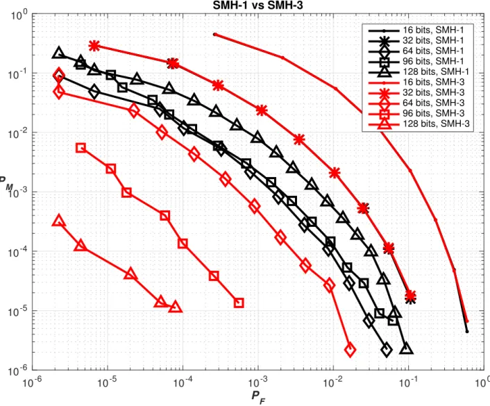
We implement Scheme 2 as SMH3. Comparing SMH3 to SMH1 and SMH2 using the synthetic dataset described in [4], we obtain the results in Figures 3.1, 3.2 and 3.3.

In this synthetic dataset, the feature dimension is fixed at d = 128 and consists of i.i.d. samples from N(0,CX). CX = UDXU where U is a

random d×d orthogonal matrix and DX is a d×d diagonal matrix with diagonal entries uniformly sampled from (0.5, 1) and normalized so that

their sum equals P = 128. The noise vector Z consists of i.i.d. samples fromN(0,CZ). CZ =VDZV whereV is a randomd×d orthogonal matrix

and DZ =diag{dz1, ..., dzd}, dzi = ar(i−1),1 ≤ i ≤ d where r = 1.05 and

Pd

i=1dzi = P. 500,000 similar pairs were generated for training in which CX and CZ were estimated and another 500,000 similar and dissimilar pairs

were generated for testing.

In Fig 3.1, we see that as the bit length increases, the improvement of SMH3 over SMH1 widens. Furthermore as the number of bits increases, SMH1 accepts more projections with low SNR and yet these projections have the same weight as those with high SNR. This causes the MAP of SMH1 to fall at bitrates higher than 64 bits. SMH3 however uses a LRT to determine the optimum weights given to each projection and is able to utilize all projections in a way to improve performance.

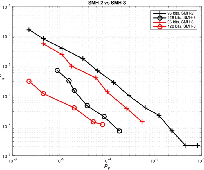
From Figure 3.2, we see that SMH3 performs consistently better than SMH2. SMH2 uses a cutoff number of projections to omit harmful projec-tions (i.e. projecprojec-tions which resulted in a decrease in MAP when included), which is not needed in SMH3 because the influence of these projections is made diminishing small. We see here that at 128 bits, SMH3 significantly outperforms SMH2 at the log scale.

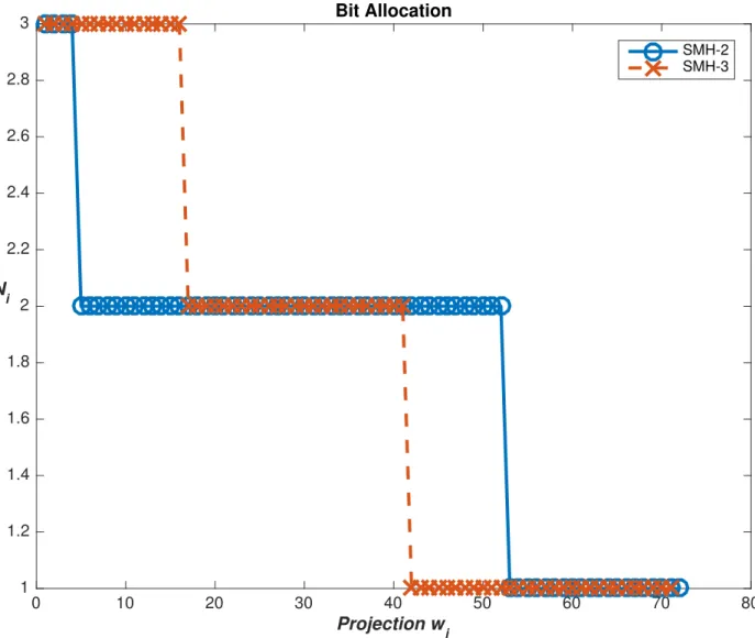
From Figure 3.3, we see that the reason SMH3 performed better was be-cause it allocated bits to the higher SNR projections much more aggressively than SMH2.

10-6 10-5 10-4 10-3 10-2 10-1 100 P_F 10-6 10-5 10-4 10-3 10-2 10-1 100 P_M SMH-1 vs SMH-3 16 bits, SMH-1 32 bits, SMH-1 64 bits, SMH-1 96 bits, SMH-1 128 bits, SMH-1 16 bits, SMH-3 32 bits, SMH-3 64 bits, SMH-3 96 bits, SMH-3 128 bits, SMH-3

10-6 10-5 10-4 10-3 10-2 P_F 10-6 10-5 10-4 10-3 10-2 10-1 P_M SMH-2 vs SMH-3 96 bits, SMH-2 128 bits, SMH-2 96 bits, SMH-3 128 bits, SMH-3

0 10 20 30 40 50 60 70 80 Projection w_i 1 1.2 1.4 1.6 1.8 2 2.2 2.4 2.6 2.8 3 N_i Bit Allocation SMH-2 SMH-3

Figure 3.3: Bit allocation comparison for SMH2 and SMH3 on synthetic data

CHAPTER 4

SNR MAXIMIZATION HASHING USING

DEEP LDA

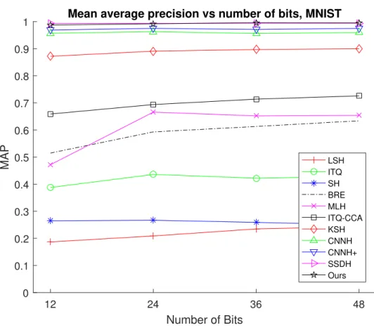
In this chapter we first introduce two recent state-of-the-art methods for semantic hashing. We then discuss the extension of using Deep LDA on SMH and how it would compare to these two state-of-the-art methods. Finally we show that on two single-label datasets, CIFAR10 and MNIST, our proposed method outperforms all compared methods.

4.1

Deep Variational and Structural Hashing

Deep Variational and Structural Hashing (DVStH) [19] uses a standard neu-ral network consisting of convolution, pooling and fully connected layers to first obtain a representative feature vector. This feature vector is used to ob-tain a probabilistic latent representation through a variational layer, where a multivariate normal distribution is fitted using Kullback-Leibler divergence as a loss function. The output of the variational block is passed through a fully-connected “struct” layer. This struct layer is split into a user-defined number of blocks and a softmax function is applied over each block. The struct layer is then split into two branches. In training, the output is sent to a fully connected “class” layer where categorical cross-entropy (CCE) loss is used as a training objective. When obtaining binary codes, the position of the maximum element in each struct block is encoded into bits and con-catenated to form the final hash code. Refer to Liong et al. [19] for more details.

4.2

Supervised Semantics-preserving Deep Hashing

stan-layers to first obtain a representative feature vector. This feature vector is passed through a fully connected layer followed by a logistic sigmoid func-tion. The size of this fully connected layer corresponds to the target bit size. The output of this layer is then used in the objective function to minimize the CCE (for the single label case) along with two terms, one encouraging the activations to be close to either 0 or 1 and the other encouraging the output of each node to have an equal probability of being 0 or 1. The output of the logistic sigmoid function is thresholded to obtain the binary hash bits. Refer to Yang et al. [20] for more details.

4.3

SMH Using Deep LDA

The original SMH method uses features from CNNs trained on CCE loss, which does not explicitly impose linear separability on the latent space rep-resentation learned by the CNN. The Deep Linear Discriminant Analysis (Deep LDA) framework [21] allows us to obtain a non-linear transformation on the input images to obtain features which are more discriminatory along the LDA directions and better fit the linear Gaussian model assumed in SMH. The LDA objective has to be reformulated to be suitable for use with the deep neural network. Particularly, two problems arise. First the estima-tion of the within-class scatter matrix overestimates high eigenvalues and underestimates small eigenvalues. Friedman [22] proposed to regularized the within-class scatter matrix with the identity matrix yielding the resultant eigenvalue problem as

Sbei =vi(SW +λI)ei, (4.1)

whereeiis the resulting eigenvector andviis the corresponding eigenvalue. Sb

and Sw are the between-class and within-class scatter matrices respectively.

Maximizing the sum of the eigenvalues tends to result in the network only maximizing the largest eigenvalue. Stuhlsatz et al. [23] tackled this via a weighted computation of the between scatter matrix, but in Dorfer et al. [21] which we follow, the sum of the k eigenvalues which do not exceed a certain threshold is maximized.

4.4

Discussion

In hashing there are three desirable properties of hash codes which we seek to achieve:

1. Uncorrelation: Individual hash bits are uncorrelated.

2. Bit balance: There is an equal chance of each bit being 0 or 1.

3. Similarity preserving: Hash code distances of similar items are lower than distances of dissimilar items.

DVStH seeks to first learn a model on the data and then instead of hashing the original inputs, seeks to hash the learned model instead. This has advan-tages in that hashing from the learned model serves as a regularization and makes the hash more robust to peculiarities of individual samples. DVStH attempts to achieve bit balance because the binarization encodes the location of the maximium element in each block. Assuming that each location has an equal chance of having the maximum element, there would be an equal chance that each bit is 0 or 1.

The use of the block softmax is a form of block-wise max-pooling and seeks to train class-specific features which are not found in other classes, for each block. Bit balance might not be achieved as it is possible that mutually exclusive features are not found or that the features in each block do not appear with equal probability. If a large struct layer is used, for example when longer bit lengths are considered, it is possible that some of the blocks are correlated as the network struggles to find discriminating projections, resulting in bits which are correlated and hence a suboptimal use of the bits allocated.

SSDH explicitly ensures bit balance in its objective function but relies on inherent design of the convolutional neural networks (CNNs) to avoid learning correlated features and hence correlated bits. However as the bit length increases, the network may possibly struggle to learn uncorrelated features leading to correlated bits.

Unlike DVStH and SSDH, the SMH method ensures bit uncorrelation be-cause of the use of the LDA which provides orthogonal projections. This ensures all of the projections used in SMH are uncorrelated, making the code as informative as possible. In terms of bit balance, for projections with

single bits, a threshold is used in SMH to ensure an equal probability of the bit being 0 or 1, but for projections with multiple bits, the binarization scheme does not ensure bit balance, but seeks to be distance-preserving.

4.5

Experimental Results

We use two datasets in our experiments. CIFAR10 [24] consists of 60,000 color images of size 32 × 32 each annotated with a single label from 10 mutually exclusive classes. The dataset is split into a training set of 50,000 images and a test set of 10,000 images. We train using the same network design and parameters in [21] except we use a batch size of 800 instead of 1000 and the number of epochs run was reduced from 10,000 to 300. Following the evaluation protocol in [19], we randomly selected 1000 samples, 100 per class, as the query set and used the remaining as the gallery set. The mean average precision (MAP) is calculated when retrieving the entire gallery set. MNIST [25] is a dataset of 70,000 28×28 grayscale images of handwritten digits annotated by a single label from 10 possible classes. It is split into 60,000 training images and 10,000 test images. We train using the same network design and parameters in [21] except we use a batch size of 800 instead of 1000. We follow the evaluation protocol of [20], randomly selecting 1000 samples from the test set and using the remaining test set as the gallery set. The MAP is calculated when retrieving the top 1000 images.

We can see that the proposed method of using SMH on top of Deep LDA outperforms all compared methods in Figures 4.1 and 4.2. If we had used 10,000 epochs as suggested in [21], instead of just 300 epochs, it is conceivable we could obtain further improvements on the CIFAR10 dataset.

12 24 36 48 Number of Bits 0 0.1 0.2 0.3 0.4 0.5 0.6 0.7 0.8 0.9 1 MAP

Mean average precision vs number of bits, CIFAR10

CNNH+ DLSHC DNNH DSRH DRSCH BDNN SuBiC ADSH DVStH Ours

12 24 36 48 Number of Bits 0 0.1 0.2 0.3 0.4 0.5 0.6 0.7 0.8 0.9 1 MAP

Mean average precision vs number of bits, MNIST

LSH ITQ SH BRE MLH ITQ-CCA KSH CNNH CNNH+ SSDH Ours

CHAPTER 5

UNSUPERVISED GRAPH

CONSTRUCTION

In this chapter we discuss some work related to unsupervised graph construc-tion and propose a binarizaconstruc-tion which allows faster graph construcconstruc-tion with similar or better results.

5.1

Notation

LetX ={x1, ..., xn} ∈Rddenote the set of features andY ={y1, ..., yn} ∈R

denote its corresponding class membership. Let xl

i denote the l-th element

of the i-th feature vector.

A graph G = (V, E, W) consists of a set of vertices V, a set of edges E which connect them, and a set of weights W which are assigned to the edges to denote the similarity between the vertices it connects. We represent the vertices as V = [x1, ..., xn] ∈ Rd×n, a matrix containing the data points

stacked column-wise. The set of edges is represented as a binary matrix E ∈ {0,1}n×n _{whose element E}

ij = 1 if there exists an edge between xi and

xj and Eij = 0 otherwise. Similarly the set of weights is represented as a

matrix W ∈_Rn×n _{whose element W}

ij denotes the similarity between xi and

xj.

5.2

Edge Learning

The k-nearest neighbors (kNN) method is possibly the most popular ap-proach to define graph topology. For each xi, kNN searches for the set

of its k nearest neighbors, Nk(xi), usually in terms of Euclidean distance.

The graph topology is defined using a symmetrization Eij = 1 if xj ∈

as the mutual kNN and better reflects manifold structure; hence it is of-ten used as a preprocessing step in state-of-the-art image manifold learning techniques.

B-matching [26] is a generalization of kNN which reformulates the edge se-lection as an optimization problem. We omit b-matching in our experiments because its O(n3_{) complexity makes it prohibitive to run on the datasets we}

use.

Other algorithms to learn a graph topology include Delaunay triangula-tion (DT) [27], and the relative neighborhood graph (RNG) [28]. These parameter-free graph construction methods however lead to deterministic graph topologies, their graph sparsity cannot be adjusted, and they are not flexible enough to capture the complex structure images have in the feature space.

5.3

Weight Learning

A popular algorithm for large scale graph construction is the anchor graph [29] [30]. Denote by U = {uk}mk=1 ⊂ Rd a set of anchor points. Each xi is

represented as a convex combination zi of the a nearest anchors of xi. We

adopt the solution used by [31] in our experiments. Let

Zij =

( exp(−kxi−ujk2/t)

P

j0∈hiiexp(−kxi−uj0k2/t), ∀j ∈ hii

0 otherwise , (5.1)

where hii ⊂[1 :m] denotes the indices of a nearest anchors of point xi inU,

and t = [1_nPn

i=1kxi −u

a_k]2_{, where u}a _{refers to the a-th nearest anchor of}

xi in the set U. The weight matrix W is recovered as W = ZΛ−1Z>, Z =

[z1, ...zn]>,Λ = diag(1>Z).

Other weight learning methods include multi-graph learning [32] [33], which combines the information from different graphs, and is especially useful when the graphs are derived from different sources.

5.4

Image Matching

Image graph construction shares similarities with image matching [34][35], where the task is to discern a link between images which are similar. In image matching, however, most of the literature is on instance level image matching, whereby the same object is in each linked image but from a different view or angle. In our work we expanded it to include semantic similarity. While the techniques might overlap to a large degree, for unsupervised semantic matching, the emphasis is on deriving information via transfer learning, and deviates from image matching algorithms which attempt to learn viewpoint, rotation and translation invariances.

We first briefly describe the scale-invariant feature transform (SIFT) [36] method which produces features worked upon by many of these image match-ing methods such as [37].

The SIFT method extracts image features by selecting a number of key patches in the images. The patches are first divided into 16 areas with eight directions in each area and a value is calculated in each direction. This re-sults in a 128-bit feature vector. As SIFT commonly generates thousands of keypoints for each image, matching via Euclidean distance becomes pro-hibitively expensive, and hence applications such as image retrieval become very time consuming.

Many research directions [37] were proposed to accelerate feature matching for SIFT, such as by improving the matching procedure of the SIFT features [38], reducing the number of SIFT keypoints [39], reducing the dimensionality of the features or binarizing these descriptors [40].

As an example of the first direction, Zhu and Wang [38] proposed a method using city-block distance and chessboard distance as the similarity metric between two feature points instead of the Euclidean distance. This draws parallels to our proposed method whereby the we introduced a similarity metric which is much faster than Euclidean distance comparison. In their method, the reduction in matching time due to the simpler matching calcu-lations results in a slight reduction in matching accuracy. Likewise in our method, we expect that there will also be a reduction in matching accuracy as some information is lost in our compression for denser datasets, but for sparse datasets we often see an improvement.

key-points. Alitappeh et al. [39] proposed to use clustering techniques to reduce the number of key points by omitting similar points. While the method im-proves the retrieval rate and reduces the matching time complexity, the clus-tering procedure adds additional processing time and the total time complex-ity may not be significantly lower. This also draws parallels to our proposed method as our proposed binarization results in a collapsed feature space, re-ducing many points with diverse feature representations in the original space to often identical binary representations in the proposed Hamming space. In a way, our proposed method does a coarse clustering of the features.

The third research direction aims to reduce the dimensionality of the image descriptors. Ke and Sukthankar [41] used principal components analysis (PCA) on the normalized gradient patches of the SIFT keypoints to obtain a smaller dimension of keypoint representation and named their method PCA-SIFT. With a lower dimensional feature vector, the feature matching time could be reduced. However, PCA-SIFT requires an offline stage to train a covariance matrix to be used for the PCA projection. A substantial amount of time might be needed for this training.

The final research direction aims to convert the features into binary rep-resentations. Ni [40] reformulated the SIFT keypoints into three diverse representations covering the inner value, the horizontal value, and the verti-cal value. Each of these representations is stored as a 128-bit code yielding a 384-bit binary string feature. Although Ni’s method obtained good matching results, and was nearly 50% more efficient than SIFT, the feature extraction time has many complex steps and may require a substantial amount of time to perform.

5.5

Proposed Method

Current unsupervised methods elucidating the relationship between images often rely heavily on the manifold structure that these images lie in the feature space. Unfortunately the high complexity of pairwise calculations and subsequent processing steps makes it difficult for these algorithms to scale up to large sample sizes, where a dense set of images in the feature space allows for the manifold techniques to work appropriately.

fea-tures of related images may be very far apart and it is hard to draw the connection between these images. Neural network features tend to perform better in these tasks because of transfer learning, whereby the semantics of a related set of images were annotated and used to train the network. A neural network trained for classification on ImageNet [42], for example, would be better positioned to represent the semantic content of images.

We propose using a thresholding of the form xl_i =_1{xl

i>0}, ∀i= 1...n, l = 1...d, (5.2)

to perform a binarization on rectified linear unit (ReLU) features pretrained with a similar dataset. This works because the ReLU only outputs a non-zero value (i.e. activated) when the neural network believes that the feature is present in the image.

Other papers have also exploited the ability of neural networks to detect features. Srivastava et al. [43] observed that different subsets of a neural network are activated for different patterns, and that a thresholding similar to Equation 5.2 of a trained neural network results in little loss of classifica-tion accuracy. Yang et al. [20] uses a hidden logistic layer to detect latent semantic concepts within images to generate binary hash codes. This feature detecting capability has however not yet been considered for unsupervised graph construction, and we show that our binarization confers better robust-ness to dataset sparsity, allows for quick computation of pairwise distances, and enables efficient storage of very large sets of unannotated features.

The proposed method is more robust to dataset sparsity in two ways. Firstly, our proposed method can be seen as a matching between images on the features they possess. This collapses the real-valued space of the original features to the smaller Hamming space, making the feature set denser without adding data points, and makes manifolds more evident and amenable to locality-sensitive methods.

Secondly, the original features have different ranges of values for each co-ordinate because normalization of the convolutional filters is not enforced. The different scales of the coordinates result in an overemphasis on certain feature coordinates when calculating distances and difficulty tracing the im-age manifold especially in sparse datasets. Our proposed method does an amplitude normalization which makes the proposed features invariant to the

scale of the convolutional filters. For these reasons, our proposed features often outperform the original features despite the significant compression, as we show in our experiments.

Furthermore the binary features allow the use of very fast XOR operations to calculate their pairwise Hamming distance, enabling larger and hence denser datasets to be used for locality-sensitive methods. This also enables larger batch sizes to be used in approximate kNN procedures and hence a better performance when these batches are pieced together. The reduction in pairwise distance computational cost reduces the main cost in kNN and related procedures.

Additionally, the compression of features into a binary form substantially reduces the storage requirements of often very large unlabelled databases.

5.6

Evaluation Metrics

Several evaluation metrics for graphs have been reported in literature. Here we adopt two intuitive task-independent evaluation metrics to assess the quality of edges and weights obtained.

Denote by accuracy = Pn i,jEij1{yi=yj} Pn i,jEij ∈[0,1] (5.3)

the fraction of obtained edges which connect two vertices of the same class membership. This is a modification of the Rand index or the “performance” measure [44], whereby accuracy only considers the edges which are detected in the graph. The reasoning is that the graphs obtained tend to be sparse and considering all possible edges makes the improvement hard to observe.

Denote by coverage = Pn i,jWij1{yi=yj} Pn i,jWij ∈[0,1] (5.4)

the fraction of the weight of all intra-class edges with respect to the total weight of all edges in the whole graph G [44].

We consider a graph to be better if it has a higher accuracy for the same number of edges obtained, or a higher coverage for the same total weight of all edges obtained [44].

5.7

Experiments

To keep our experiments tractable, we restrict the size of datasets to 10k datapoints. We use the test sets of CIFAR10 [24], MNIST [25], MNIST Fashion [45], STL-10 [46], CALTECH-101 [47], and the first 10k images from the test set of SVHN [48]. The two face classes in CALTECH-101 are merged and the background class was omitted. The 4096-dimensional features are derived from the ReLU6 layer of imagenet-vgg-m-128 [49], a neural network pretrained for the purpose of producing transferable features. The choice of using the penultimate ReLU is to expand the number of features which could be matched.

Our experiments show improvements in some of the most popular graph construction methods with our binarization approach as compared to using the original features. We elect to use kNN and anchor graphs to showcase these improvements as they are the most frequently used, and are the foun-dation for more sophisticated algorithms.

Figure 5.1 shows the accuracy against number of retrieved pairs using the original features in Euclidean space and using our proposed approach with Hamming distance on mutual kNN. We see that our proposed method does similar or better than using the original features, in all six datasets.

Figure 5.2 shows the accuracy of the k-nearest neighbors against the num-ber of neighbors retrieved. In this case accuracy reflects the fraction of re-trieved neighbors which are of the same class as the node on which kNN is done. The figure shows that the proposed method does similar or bet-ter than using the original features in Euclidean space, signifying a slightly higher robustness to reconstruction methods which are not locality-sensitive, and hence allows the use of faster global reconstruction algorithms.

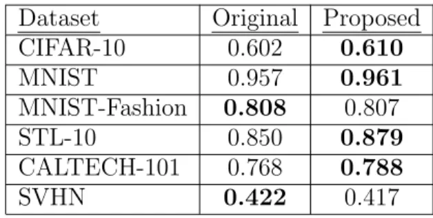
Table 5.1 shows the coverage when the anchor graph algorithm of Section 5.3 is used, with m = 3000 and a = 2, using both the original features and the proposed features. The best performance is shown in bold and it can be seen that the proposed approach performs similarly to or slightly better than using the original features, on most datasets. This indicates that the proposed method could be used as a low memory storage cost alternative in global reconstruction methods.

Table 5.1: Coverage of anchor graphs using original features and proposed method. Total weight sum is 10k in each case.

Dataset Original Proposed

CIFAR-10 0.602 0.610 MNIST 0.957 0.961 MNIST-Fashion 0.808 0.807 STL-10 0.850 0.879 CALTECH-101 0.768 0.788 SVHN 0.422 0.417

5.8

Discussion

We here present an alternative view on why the binarized features can pro-duce even better accuracy than the original features using Euclidean dis-tance metrics, despite substantial compression, when the dataset is sparse. In his doctoral dissertation [50], Yu showed that under the Gaussian model, the Hamming metric is more robust to decreases in SNR than the Euclidean metric. Specifically Yu showed that Hamming distance on hash codes trained with SMH outperforms Euclidean nearest neighbors in the low-SNR regime. Our binarized features are analogous to a 4096-bit hash code trained by SMH, as all of the features trained were ideally distinct and can be seen as orthogonal projections.

When the amount of data available is low, the noise could be relatively high because the variance of similar samples on each coordinate could be high by chance. This is conceivably more stable when more data is available, resulting in a higher SNR. Hence when data is sparse, our binarized features could exist in the low-SNR regime and hence perform better than using the original features with Euclidean metrics.

0 2 4 6 8 10 Number of Pairs obtained ×104

0 0.1 0.2 0.3 0.4 0.5 0.6 0.7 0.8 0.9 1 Accuracy Euclidean Proposed (a) CIFAR10 0 0.5 1 1.5 2 2.5 3

Number of Pairs obtained ×105

0 0.1 0.2 0.3 0.4 0.5 0.6 0.7 0.8 0.9 1 Accuracy Euclidean Proposed (b) MNIST 0 0.5 1 1.5 2 2.5

Number of Pairs obtained ×105 0 0.1 0.2 0.3 0.4 0.5 0.6 0.7 0.8 0.9 1 Accuracy Euclidean Proposed (c) MNIST Fashion 0 2 4 6 8 10 12

Number of Pairs obtained ×104 0 0.1 0.2 0.3 0.4 0.5 0.6 0.7 0.8 0.9 1 Accuracy Euclidean Proposed (d) STL-10 0 2 4 6 8 10 12 14

Number of Pairs obtained ×104

0 0.1 0.2 0.3 0.4 0.5 0.6 0.7 0.8 0.9 1 Accuracy Euclidean Proposed (e) CALTECH-101 0 0.5 1 1.5 2

Number of Pairs obtained ×105

0 0.1 0.2 0.3 0.4 0.5 0.6 0.7 0.8 0.9 1 Accuracy Euclidean Proposed (f) SVHN Figure 5.1: Accuracy of edges derived by mutual neighbors.

0 20 40 60 80 100 Number of Neighbors retrieved

0 0.1 0.2 0.3 0.4 0.5 0.6 0.7 0.8 0.9 1 Accuracy Euclidean Proposed (a) CIFAR10 0 20 40 60 80 100 Number of Neighbors retrieved

0 0.1 0.2 0.3 0.4 0.5 0.6 0.7 0.8 0.9 1 Accuracy Euclidean Proposed (b) MNIST 0 20 40 60 80 100 Number of Neighbors retrieved

0 0.1 0.2 0.3 0.4 0.5 0.6 0.7 0.8 0.9 1 Accuracy Euclidean Proposed (c) MNIST Fashion 0 20 40 60 80 100 Number of Neighbors retrieved

0 0.1 0.2 0.3 0.4 0.5 0.6 0.7 0.8 0.9 1 Accuracy Euclidean Proposed (d) STL-10 0 20 40 60 80 100 Number of Neighbors retrieved

0 0.1 0.2 0.3 0.4 0.5 0.6 0.7 0.8 0.9 1 Accuracy Euclidean Proposed (e) CALTECH-101 0 20 40 60 80 100 Number of Neighbors retrieved

0 0.1 0.2 0.3 0.4 0.5 0.6 0.7 0.8 0.9 1 Accuracy Euclidean Proposed (f) SVHN

Figure 5.2: Average accuracy of the k-nearest neighbors against the number of neighbors retrieved.

CHAPTER 6

FUTURE WORK AND DISCUSSION

6.1

Extension of SMH to Multilabel Datasets

The Deep LDA model used with SMH currently only supports single label datasets. It should be possible to extend it to the multilabel case, for example by using Multi-Label LDA [51], which produces between-class and within-class scatter matrices analogous to the standard LDA scatter matrices. These multi-label scatter matrices could be used in place of the original scatter matrices to extend Deep LDA for the multi-label case.

6.2

Uunsupervised Learning Evaluation

In our evaluation metric, the correct class demarcation is determined by the labels. Consider the images in Figure 6.1 which are taken from the SVHN [48] dataset and two corresponding partitions in red and blue. We can see that both partitions can be justified. The red partition splits the images into the number it represents; the blue partition splits the images into the style it possesses. However, in the evaluation metrics used, the red partition is correct and the blue partition is wrong. The choice of which partition is “correct” can only be determined by the labels.

In this pretraining, features which best distinguish between images of these labels were trained. When a different type of label is subsequently used, the trained features may be poor in distinguishing between images of the new label. In the example of Figure 6.1, suppose the neural network was trained to distinguish between styles. The features it produces will detect elements of style and the images grouped by the blue partition will be closer in the original feature space.

Figure 6.1: Images taken from the SVHN dataset [48]. The red partition splits the images into the number it represents; the blue partition splits the images into the style it possesses.

In many experiments, a much better result for unsupervised learning could be obtained simply by choosing a more similar dataset to pretrain the neural network with. In our experiments we obviated the need to control for this by simply showing that our proposed binarization performs similarly to or better than the original features in sparse datasets, using the same pretrained network.

Had some labels been available (i.e. for semi-supervised learning), it would be much easier to guide the network towards the discriminations desired by the labels.

6.3

Microscopic Structure

A key goal in unsupervised learning is to recognize patterns from unlabelled data. Using the features from a particular neural network would only provide information about the concepts the neural network was trained to distinguish. Combining the information from features trained by different networks would give a more complete picture of the relationship between the images.

The proposed method could be used to provide such a building block. In Wang et al. [52] for example, the community structure (using community de-tection methods) and the microscopic structure (using proximity information [53]) were incorporated to generate a network embedding. Calculating the microscopic structure has very high complexity and is intractable for large datasets. Using our proposed method, this microscopic structure can be cal-culated quickly and can be used in applications where proximity information is needed.

CHAPTER 7

CONCLUSION

We have shown an improvement to the bit allocation strategy of Signal-to-Noise Ratio Maximization Hashing and extended it to use a Deep Linear Discriminant Analysis method to obtain features. The proposed method was shown to outperform all compared state-of-the-art methods.

We have also shown a method to binarize sparse image features and re-port similar or often better performance than using original features on mu-tual kNN, while requiring much lower computational and storage resources. Furthermore we analyze how our binarization is robust to dataset sparsity. Specifically when data is sparse, the signal-to-noise ratio declines, which de-creases the discriminatory ability of the Euclidean metric faster than the Hamming metric.

REFERENCES

[1] J. Wang, T. Zhang, J. Song, N. Sebe, and H. T. Shen, “A survey on learning to hash,” arXiv preprint arXiv:1606.00185, 2016.

[2] H. Jegou, M. Douze, and C. Schmid, “Product quantization for nearest neighbor search,”IEEE Transactions on Pattern Analysis and Machine

Intelligence, vol. 33, no. 1, pp. 117–128, 2011.

[3] A. W. Smeulders, M. Worring, S. Santini, A. Gupta, and R. Jain, “Content-based image retrieval at the end of the early years,” IEEE

Transactions on Pattern Analysis and Machine Intelligence, vol. 22,

no. 12, pp. 1349–1380, 2000.

[4] H. Yu and P. Moulin, “SNR maximization hashing,”IEEE Transactions

on Information Forensics and Security, vol. 10, no. 9, pp. 1927–1938,

2015.

[5] H. Jain, J. Zepeda, P. P´erez, and R. Gribonval, “Learning a complete image indexing pipeline,” arXiv preprint arXiv:1712.04480, 2017. [6] J. Sivic and A. Zisserman, “Video google: A text retrieval approach

to object matching in videos,” in IEEE International Conference on

Computer Vision, 2003, p. 1470.

[7] H. Jain, J. Zepeda, P. P´erez, and R. Gribonval, “SUBIC: A supervised, structured binary code for image search,” in Proc. Int. Conf. Computer

Vision, vol. 1, no. 2, 2017, p. 3.

[8] M. S. Charikar, “Similarity estimation techniques from rounding algo-rithms,” in Proceedings of the Thirty-Fourth Annual ACM Symposium

on Theory of Computing. ACM, 2002, pp. 380–388.

[9] H. Jegou, “Efficient similarity search,” in Frontiers of Multimedia

Re-search, 2018, pp. 105–134.

[10] Y. Weiss, A. Torralba, and R. Fergus, “Spectral hashing,” in Advances

[11] Y. Gong, S. Lazebnik, A. Gordo, and F. Perronnin, “Iterative quanti-zation: A procrustean approach to learning binary codes for large-scale image retrieval,” IEEE Transactions on Pattern Analysis and Machine

Intelligence, vol. 35, no. 12, pp. 2916–2929, 2013.

[12] F. Zhao, Y. Huang, L. Wang, and T. Tan, “Deep semantic ranking based hashing for multi-label image retrieval,” inProceedings of the IEEE

Con-ference on Computer Vision and Pattern Recognition, 2015, pp. 1556–

1564.

[13] K. Lin, H.-F. Yang, J.-H. Hsiao, and C.-S. Chen, “Deep learning of binary hash codes for fast image retrieval,” in Proceedings of the IEEE

Conference on Computer Vision and Pattern Recognition Workshops,

2015, pp. 27–35.

[14] H. Liu, R. Wang, S. Shan, and X. Chen, “Deep supervised hashing for fast image retrieval,” in Proceedings of the IEEE Conference on

Com-puter Vision and Pattern Recognition, 2016, pp. 2064–2072.

[15] J. Wang, H. T. Shen, J. Song, and J. Ji, “Hashing for similarity search: A survey,” arXiv preprint arXiv:1408.2927, 2014.

[16] T. Yao, F. Long, T. Mei, and Y. Rui, “Deep semantic-preserving and ranking-based hashing for image retrieval.” in IJCAI, 2016, pp. 3931– 3937.

[17] J. Wang, W. Liu, A. X. Sun, and Y.-G. Jiang, “Learning hash codes with listwise supervision,” in Proceedings of the IEEE International

Confer-ence on Computer Vision, 2013, pp. 3032–3039.

[18] T. Zhang, C. Du, and J. Wang, “Composite quantization for approxi-mate nearest neighbor search,” in ICML, no. 2, 2014, pp. 838–846. [19] V. E. Liong, J. Lu, L.-Y. Duan, and Y. Tan, “Deep variational and

structural hashing,” IEEE Transactions on Pattern Analysis and

Ma-chine Intelligence, 2018.

[20] H.-F. Yang, K. Lin, and C.-S. Chen, “Supervised learning of semantics-preserving hash via deep convolutional neural networks,” IEEE

Trans-actions on Pattern Analysis and Machine Intelligence, vol. 40, no. 2, pp.

437–451, 2018.

[21] M. Dorfer, R. Kelz, and G. Widmer, “Deep linear discriminant analysis,” arXiv preprint arXiv:1511.04707, 2015.

[22] J. H. Friedman, “Regularized discriminant analysis,” Journal of the

[23] A. Stuhlsatz, J. Lippel, and T. Zielke, “Feature extraction with deep neural networks by a generalized discriminant analysis,” IEEE

trans-actions on Neural Networks and Learning Systems, vol. 23, no. 4, pp.

596–608, 2012.

[24] A. Krizhevsky and G. Hinton, “Learning multiple layers of features from tiny images,” University of Toronto, Tech. Rep., 2009.

[25] Y. LeCun, C. Cortes, and C. Burges, “MNIST handwritten digit database,” AT&T Labs [Online]. Available: http://yann. lecun. com/exdb/mnist, 2010.

[26] T. Jebara and V. Shchogolev, “B-matching for spectral clustering,” in

European Conference on Machine Learning. Springer, 2006, pp. 679–

686.

[27] D.-T. Lee and B. J. Schachter, “Two algorithms for constructing a De-launay triangulation,” International Journal of Computer &

Informa-tion Sciences, vol. 9, no. 3, pp. 219–242, 1980.

[28] K. J. Supowit, “The relative neighborhood graph, with an application to minimum spanning trees,” Journal of the ACM (JACM), vol. 30, no. 3, pp. 428–448, 1983.

[29] W. Liu, J. He, and S.-F. Chang, “Large graph construction for scal-able semi-supervised learning,” in Proceedings of the 27th International

Conference on Machine Learning (ICML-10), 2010, pp. 679–686.

[30] W. Liu, J. Wang, S. Kumar, and S.-F. Chang, “Hashing with graphs,” in

Proceedings of the 28th International Conference on Machine Learning

(ICML-11). Citeseer, 2011, pp. 1–8.

[31] F. Shen, Y. Xu, L. Liu, Y. Yang, Z. Huang, and H. T. Shen, “Unsuper-vised deep hashing with similarity-adaptive and discrete optimization,”

IEEE Transactions on Pattern Analysis and Machine Intelligence, 2018.

[32] W. Tang, Z. Lu, and I. S. Dhillon, “Clustering with multiple graphs,”

inData Mining, 2009. ICDM’09. Ninth IEEE International Conference

on. IEEE, 2009, pp. 1016–1021.

[33] B. Wang, J. Jiang, W. Wang, Z.-H. Zhou, and Z. Tu, “Unsupervised metric fusion by cross diffusion,” inComputer Vision and Pattern

Recog-nition (CVPR), 2012 IEEE Conference on. IEEE, 2012, pp. 2997–3004.

[34] K. Heath, N. Gelfand, M. Ovsjanikov, M. Aanjaneya, and L. J. Guibas, “Image webs: Computing and exploiting connectivity in image collec-tions,” 2010 IEEE Computer Society Conference on Computer Vision

[35] S. Agarwal, N. Snavely, I. Simon, S. M. Seitz, and R. Szeliski, “Building rome in a day,” in Computer Vision, 2009 IEEE 12th International

Conference on. IEEE, 2009, pp. 72–79.

[36] D. G. Lowe, “Distinctive image features from scale-invariant keypoints,”

International Journal of Computer Vision, vol. 60, no. 2, pp. 91–110,

2004.

[37] C.-C. Chen and S.-L. Hsieh, “Using binarization and hashing for ef-ficient SIFT matching,” Journal of Visual Communication and Image

Representation, vol. 30, pp. 86–93, 2015.

[38] D. Zhu and X. Wang, “A method of improving SIFT algorithm matching efficiency,” in Image and Signal Processing, 2009. CISP’09. 2nd

Inter-national Congress on. IEEE, 2009, pp. 1–5.

[39] R. J. Alitappeh, K. J. Saravi, and F. Mahmoudi, “Key point reduc-tion in SIFT descriptor used by subtractive clustering,” in Information Science, Signal Processing and their Applications (ISSPA), 2012 11th

International Conference on. IEEE, 2012, pp. 906–911.

[40] Z.-S. Ni, “B-SIFT: a binary SIFT based local image feature descrip-tor,” in Digital Home (ICDH), 2012 Fourth International Conference on. IEEE, 2012, pp. 117–121.

[41] Y. Ke and R. Sukthankar, “PCA-SIFT: A more distinctive represen-tation for local image descriptors,” in Computer Vision and Pattern Recognition, 2004. CVPR 2004. Proceedings of the 2004 IEEE

Com-puter Society Conference on, vol. 2. IEEE, 2004, pp. II–II.

[42] J. Deng, W. Dong, R. Socher, L.-J. Li, K. Li, and F.-F. Li, “ImageNet: A large-scale hierarchical image database,” in CVPR09, 2009.

[43] R. K. Srivastava, J. Masci, F. Gomez, and J. Schmidhuber, “Under-standing locally competitive networks,” arXiv preprint arXiv:1410.1165, 2014.

[44] H. Almeida, D. Guedes, W. Meira, and M. J. Zaki, “Is there a best quality metric for graph clusters?” in Joint European Conference on

Machine Learning and Knowledge Discovery in Databases. Springer,

2011, pp. 44–59.

[45] H. Xiao, K. Rasul, and R. Vollgraf, “Fashion-MNIST: a novel image dataset for benchmarking machine learning algorithms,” arXiv preprint arXiv:1708.07747, 2017.

[46] A. Coates, A. Ng, and H. Lee, “An analysis of single-layer networks in unsupervised feature learning,” in Proceedings of the Fourteenth

Inter-national Conference on Artificial Intelligence and Statistics, 2011, pp.

215–223.

[47] F.-F. Li, R. Fergus, and P. Perona, “Learning generative visual models from few training examples: An incremental Bayesian approach tested on 101 object categories,” Computer Vision and Image Understanding, vol. 106, no. 1, pp. 59–70, 2007.

[48] Y. Netzer, T. Wang, A. Coates, A. Bissacco, B. Wu, and A. Y. Ng, “Reading digits in natural images with unsupervised feature learning,”

in NIPS Workshop on Deep Learning and Unsupervised Feature

Learn-ing, vol. 2011, no. 2, 2011, p. 5.

[49] K. Chatfield, K. Simonyan, A. Vedaldi, and A. Zisserman, “Return of the devil in the details: Delving deep into convolutional nets,” inBritish

Machine Vision Conference, 2014.

[50] H. Yu, “Learning compact hashing codes for large-scale similarity search,” Ph.D. dissertation, University of Illinois at Urbana-Champaign, 2015.

[51] H. Wang, C. Ding, and H. Huang, “Multi-label linear discriminant anal-ysis,” in European Conference on Computer Vision. Springer, 2010, pp. 126–139.

[52] X. Wang, P. Cui, J. Wang, J. Pei, W. Zhu, and S. Yang, “Community preserving network embedding,” in AAAI, 2017, pp. 203–209.

[53] J. Tang, M. Qu, M. Wang, M. Zhang, J. Yan, and Q. Mei, “Line: Large-scale information network embedding,” inProceedings of the 24th

Inter-national Conference on World Wide Web. International World Wide