Bayesian Learning of Asymmetric Gaussian-Based Statistical Models using Markov Chain Monte Carlo Techniques

(1)

Bayesian Learning of Asymmetric Gaussian-Based

Statistical Models using Markov Chain Monte Carlo

Techniques

Shuai Fu

A Thesis in

The Concordia Institute for

Information Systems Engineering

Presented in Partial Fulfillment of the Requirements for the Degree of

Master of Applied Science (Information Systems Security) at Concordia University

Montr´eal, Qu´ebec, Canada

July 2018

c

(2)

CONCORDIA

UNIVERSITY

School of Graduate Studies

This is to certify that the thesis prepared

By: Shuai Fu

Entitled: Bayesian Learning of Asymmetric Gaussian-Based Statistical Models

using Markov Chain Monte Carlo Techniques

and submitted in partial fulfillment of the requirements for the degree of

Master of Applied Science (Information Systems Security)

complies with the regulations of this University and meets the accepted standards with respect to originality and quality.

Signed by the Final Examining Committee:

Chair Dr. Amr Youssef External Examiner Dr. Joonhee Lee Examiner Dr. Jamal Bentahar Supervisor Dr. Nizar Bouguila Approved by

Amr Youssef, Chair

Department of Information Systems Engineering

2018

Amir Asif, Dean

(3)

Abstract

Bayesian Learning of Asymmetric Gaussian-Based Statistical Models using Markov Chain Monte Carlo Techniques

Shuai Fu

A novel unsupervised Bayesian learning framework based on asymmetric Gaussian mixture (AGM) statistical model is proposed since AGM is shown to be more effective compared to the classic Gaussian mixture. The Bayesian learning framework is developed by adopting sampling-based Markov chain Monte Carlo (MCMC) methodology. More precisely, the fundamental learning algorithm is a hybrid Metropolis-Hastings within Gibbs sampling solution which is integrated within a reversible jump MCMC (RJMCMC) learning framework, a self-adapted sampling-based MCMC implementation, that enables model transfer throughout the mixture parameters learning process, therefore, automatically converges to the optimal number of data groups. Furthermore, a feature selection technique is included to tackle the irrelevant and unneeded information from datasets. The performance comparison between AGM and other popular solutions is given and both synthetic and real data sets extracted from challenging applications such as intrusion detection, spam filtering and image categorization are evaluated to show the merits of the proposed approach.

(4)

Acknowledgments

I would like to firstly express my gratitude to my supervisor Dr. Nizar Bouguila not only for his important academic guidance and suggestions throughout the study of my Master program but also for his personal concerns and continuous supports to me and my family. I could not image that I could graduate from the program without his endless patience, warm encourage and financial supports. What I am learning from him will definitely influences my entire life.

I also want to extend my gratefulness to all the professors and colleagues of Concordia Institute for Information Systems Engineering to providing this great opportunity to learning with the most talented supervisors and students in Concordia University.

Finally, I would like to thank my parents and my wife for their persistent and unconditional love and support, and my daughter, for the happiness she brought to my family.

(5)

List of Figures

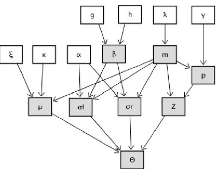
Figure 2.1 DAG of RJMCMC parameter learning Bayesian network . . . 16

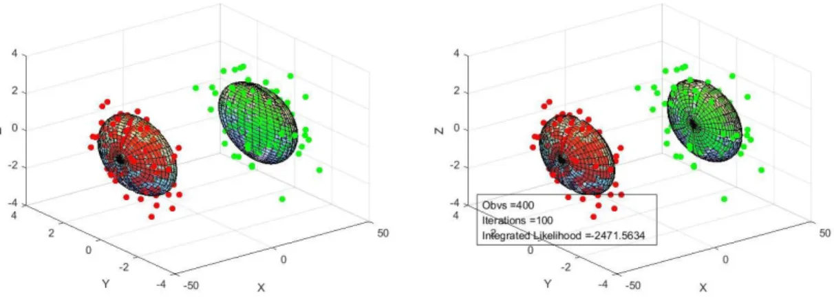
Figure 2.2 Original synthetic data grouping and learning results. . . 17

Figure 2.3 (a) Original synthetic data grouping; (b) AGM clustering results . . . 18

Figure 3.1 DAG of AGM Bayesian learning network with feature selection. . . 29

Figure 3.2 a) Original UIUC sport image. b) Enhanced image with SIFT extracted visual features. . . 30

Figure 3.3 a) Clustering accuracy by vocabulary size. b) Clustering accuracy by latent aspect number. . . 30

Figure 3.4 Confusion matrix of AGM model (Vocabulary size is 1000 and latent aspect number is 30) . . . 31

(8)

List of Tables

Table 2.1 AGM Learning Statistics . . . 19

Table 2.2 Accuracy Analysis (M0 ₌_M _{= 2)} _{. . . .} ₁₉ Table 2.3 Original NSL-KDD data records . . . 21

Table 2.4 Translation and Normalization of Internet Protocols (Enumerated Values) . . 22

Table 2.5 Confusion Matrices and Statistics of K-means, GMM and AGM Models . . . 22

Table 2.6 AGM Statistics . . . 23

(9)

Chapter 1

Introduction

1.1 Introduction

Over past decades, many statistical data mining approaches have been proposed to address chal-lenging data modeling analysis problems given the fact that the volume of data is dramatically increasing due to the usage of Internet. Meanwhile, modern machine-learning-based techniques perform in both generative and discriminative ways which can be divided into two main streams, classification-based supervised and clustering-based unsupervised ones. Compared to supervised solutions, unsupervised approach has no assumption on the number of groups, therefore, friendly to newly added data and patterns which makes it more suitable for increasing database analysis. Moreover, it also immunizes against learning biases and overfitting problems that commonly exist in most supervised approaches if model training is inappropriate. Consequently, there has been an increasing trend of applying finite mixtures into different domains involving statistical modeling of data, such as astronomy, ecology, bioinformatics, pattern recognition, computer vision and machine

learning [1]. Our work is based on asymmetric Gaussian mixture (AGM) model [2] and reversible

jump Markov chain Monte Carlo (RJMCMC) learning algorithm [3]. Previous efforts reveal the

fact that AGM outperforms classic Gaussian mixture model (GMM) by taking asymmetric datasets

into consideration which provides more flexibility [4]. Our RJMCMC implementation is based on

a hybrid sampling-based approach which takes advantages of both Metropolis-Hastings (MH) and

Gibbs sampling methods [5], therefore, simplifies mathematical complexity and extends

(10)

applies a dynamic data-based strategy to identify the optimal components number throughout iter-ations which makes the model learning a self-adaptive process. To achieve better fitting outcomes, feature selection process is involved to handle high-dimensional vectors of features and the analysis and discussion of deploying AGM to both synthetic datasets and real applications is given in the later chapters.

1.1.1 Finite Mixture Models

As upgrade of single-mathematical-model-based methodologies, mixture models [6,7, 8] can

be seen as a superimposition of certain mixture components sharing dependencies with each other, therefore, lead to outstanding performance especially for high-dimensional and multi-cluster datasets. Finite mixture models can be described by

p(X|Θ) =

M X

j=1

pjp(X|Θj) (1)

whereX reprensents a vector in a given dataset andΘdefines the mixture parameters set (for

each mixture compoent, the sub-parameter set is described byΘj, j = 1, . . . , M) as well as

com-ponent weightpj (0< pj ≤1 andPMj=1pj = 1).

1.1.2 Probability Density Function Selection

Probability density function (PDF) selection has an important role in finite mixture model be-cause it significantly affects the capability of representing the data. Improper PDF selection will cause incorrect outcomes such as wrong components number and poor data fitting. Gaussian

mix-ture model (GMM) [3] demonstrated satisfactory fitting abilities on most real applications whose

datasets are Gaussian-like. However, under more general circumstances regarding to non-Gaussian

or asymmetric datasets, asymmetric Gaussian mixture (AGM) model [2] leads to a better

accu-racy by introducing two variance parameters for both left and right parts of asymmetric Gaussian distribution, providing more flexibility for variant real applications. Therefore, the justification of choosing AGM model and its merits will be discussed in the following chapters.

(11)

1.1.3 Bayesian Learning Framework

Estimating the parameters of mixture models could be a challenging task. The

maximum-likelihood-based expectation maximization (EM) [9] algorithm is one of the most popular parameter

learning approaches. However, the disadvantages of EM algorithm are also obvious. Given the fact that EM approximates values of mixture parameters in a deterministic way this could cause slow convergence and compromise the usability of the algorithm. Furthermore, bad initialization and

overfitting problems [10,11] will also significantly affect its accuracy. Therefore, fully Bayesian

learning algorithms, such as Markov Chain Monte Carlo (MCMC) based implementations, are found to be useful to eliminate overfitting problems in mixture parameter learning by introduc-ing prior and posterior distributions for mixture parameters. In our work, the learnintroduc-ing process is accomplished by a hybrid MCMC algorithm, which is well known as Metropolis-Hastings within

Gibbs sampling [10,12], based on both Metropolis-Hastings [13] and Gibbs sampling [14] methods

because the main difficulty of classic MCMC method is that, under some circumstances, direct sam-pling is not always straightforward. Moreover, we reinforce the learning algorithm by introducing

reversible jump MCMC (RJMCMC) [3] methodology to increase the flexibility of AGM model by

allowing model transfer throughout iterations via increasing (component birth/split step) and de-creasing (component death/merge step) mixture components. Because of the stochastic sampling-based learning process, learning iterations could end up with different number of components so

we choose marginal likelihood [10] to perform model selection in order to evaluate fitting results

between models.

1.1.4 Dimensionality Reduction

One of the most important tasks in data mining, pattern recognition, computer vision and ma-chine learning applications is that, the existence of outliers and irrelevant features severely compro-mises the clustering outcomes. Therefore, many dimensionality reduction methodologies have been

proposed [15,16] such as feature extraction and selection which try to remove these unneeded

fea-tures in order to improve the performance of the modeling [17,18] while feature extraction is based

on transformations or combinations of the original features [19]. Indeed, feature selection

(12)

[20,21] has shown that selecting relevant features leads to more accurate modeling results. How-ever, this problem is not trivial especially in the unsupervised context dealing with labelless data

sets. For this reason, previous researches [22,4,23] were devoted to extend unsupervised feature

selection to mixture-based clustering. In this thesis, we extended the RJMCMC-based simultaneous

Bayesian clustering and feature selection approach proposed in [4] to asymmetric Gaussian

mix-ture model in order to improve the modeling performance on a challenging image categorization application.

1.2 Contributions

The contributions of this thesis are as follows:

+ A Novel Bayesian Framework for Asymmetric Gaussian Mixture via Markov Chain Monte Carlo Method:We chose an advanced MCMC implementation called reversible jump

MCMC (RJMCMC) [11] which is based on a hybrid Metropolis-Hastings within Gibbs

sam-pling [10] solution, combining both Metropolis-Hastings [13] and Gibbs sampling [14]

meth-ods because the main difficulty of applying traditional MCMC method is that, under some circumstances, direct sampling is not always straightforward that distributions of mixture pa-rameters are latent and dependencies between papa-rameters are unknown. By integrating the merits of both methods, mixture parameters will be evaluated iteratively and, eventually, the optimal parameter values will be identified after convergence. Furthermore the self-adapted

learning process [11] treats components number as an extra parameter and adjusts it

through-out iterations by automatically increasing (component birth/death step) and decreasing (com-ponent merge/split step) according to current status, therefore, enables model transfer which significantly improves the learning performance. This contribution has been published in [24].

+ Intrusion Detection and Spam Filtering by Applying Proposed Approach via Reversible Jump MCMC:We apply and adapt the proposed Bayesian learning framework to two

chal-lenging applications namely intrusion detection and spam filtering ([25] and [26]).

+ Feature Selection for Image Categorization: While deploying the proposed approach for image categorization, in order to better identify visual features from the challenging UIUC

(13)

sport events dataset, the image representative data is generated by adopting scale-invariant feature transform (SIFT), bag-of-visual-words (BOVW) and probabilistic latent semantic analysis (pLSA) techniques. However, previous approaches assume all the features of ob-servations have the same weight of importance and carry pertinent information which is not always the case and many of those features can be irrelevant for clustering purpose. In or-der to tackle this problem and define relevance and importance of features, feature selection

techniques [4,23] should be taken into consideration. Eventually, irrelevant and unneeded

information will be filtered by feature selection.

1.3 Thesis Overview

The rest of this thesis is organized as follows:

o Chapter 2 introduces the Asymmetric Gaussian mixture model and its sampling based Bayesian

learning framework. In particular, a self-adapted reversible jump MCMC implementation which has no assumption concerning the number of components and, therefore, the AGM model itself could be transferred between iterations. Furthermore the self-adapted learn-ing process treats components number as an extra parameter and adjusts it throughout iter-ations by automatically increasing (component birth/death step) and decreasing (component merge/split step) according to current status, therefore, enables model transfer which signifi-cantly improves the learning performance.

o Chapter 3 is devoted to feature selection since the AGM model assumes that all the features

of observations have the same weight of importance and carry pertinent information which is not always the case and many of those features can be irrelevant for clustering purpose. In order to tackle this problem and define relevance and importance of features, feature selection techniques should be taken into consideration. A challenging UIUC sports event database is selected for validation of the proposed approach.

(14)

Chapter 2

Asymmetric Gaussian Mixtures with

Reversible Jump MCMC and

Applications

This chapter presents a novel intrusion detection classifier based on asymmetric Gaussian mix-ture (AGM) model and reversible jump Markov chain Monte Carlo (RJMCMC) learning algorithm. Previous efforts reveal the fact that AGM outperforms classic Gaussian mixture model (GMM) by taking asymmetric datasets into consideration which provides more flexibility. Our RJMCMC implementation is based on a hybrid sampling-based approach which takes advantages of both Metropolis-Hastings (MH) and Gibbs sampling methods, therefore, simplifies mathematical com-plexity and extends adaptability of the model. Moreover, without giving a fixed components num-ber in advance, RJMCMC applies a dynamic data-based strategy to identify the optimal compo-nents number throughout iterations which makes the model learning a self-adaptive process. Since the model is nondeterministic, Laplace approximation based marginal likelihood is calculated for multiple runs as model selection procedure to improve the correctness and fitting accuracy. Both synthetic and real datasets are applied to our model to discover its merits and the test results will be evaluated and compared with other popular solutions.

(15)

2.1 Asymmetric Gaussian Mixture Model

The likelihood function of AGM model [2] withM mixture components can be illustrated as

follows: p(X |Θ) = N Y i=1 M X j=1 pjp(Xi|ξj) (2)

whereX = (X1, ..., XN)reprensents the dataset withNobservations,Θ ={p1, ..., pM, ξ1, ..., ξM}

defines the mixture parameters set of AGM mixture model including component weight pj (0

< pj ≤1 and PMj=1pj = 1) and asymmetric Gaussian distribution (AGD) parameters set ξj for

mixture component j. Assuming the dataset X is d-dimensional, for each observation Xn =

(xn1, ..., xnd) ∈ X, the probability density function [2] for j-th component of the model can be defined as follows: p(X|ξj)∝ d Y k=1 1 (σljk +σrjk) ×        exp −(xk−µjk)2 2(σ_ljk)2 if xk < µjk exp −(xk−µjk)2 2(σ_rjk)2 if xk > µjk (3)

parameters set of component j isξj = (µj, σlj, σrj) where µj = (µj1, ..., µjd) is the mean,

σlj = (σlj1, ..., σljd) and σrj = (σrj1, ..., σrjd) represents the left and right standard deviation vectors of AGD .

We bring aM-dimensional membership vectorZto each observationXi ∈ X, Zi = (Zi1, ..., ZiM),

indicating which specific componentXibelongs to [1], such that:

Zij =    1 ifXibelongs to componentj 0 otherwise (4)

that being said, Zij = 1 only when observationXi has the highest probability of belonging to

componentjand accordingly, for other components,Zij = 0.

(16)

follows: p(X, Z|Θ) = N Y i=1 M Y j=1 (pjp(Xi|ξj))Zij (5)

2.2 Bayesian Learning Algorithm

Before describing MH-within-Gibbs learning steps, the priors and posteriors need to be

speci-fied. First, we denote the postorior probability of membership vector Z asπ(Z|Θ,X)[5]:

Z(t)∼π(Z|Θ(t−1)_,_X₎ ₍₆₎

the number of observations belonging to a specific component j can be calculated using Z(t) as

follows: n(_jt)= N X i=1 Zij (j= 1, ..., M) (7)

thusn(t) = (n₁(t), ..., n(_Mt))represents the number of observations belonging to each mixture compo-nent.

Since the mixture weightpj satisfies the following conditions (0< pj ≤1 andPMj=1pj = 1), a

natural choice of the prior is Dirichlet distribution as follows [27,28]

π(p1, . . . , pM)∼ D(γ1, ..., γM) (8)

whereγjis known hyperparameter. Consequently, the posterior of the mixture weightpj is:

p(p1, . . . , pM|Z(t))∼ D(γ1+n(1t), ..., γM +n( t)

M) (9)

Direct sampling of mixture parametersξ ∼p(ξ|Z,X)could be difficult so Metropolis-Hastings

method should be deployed using proposal distributions forξ(t)_∼_q₍_ξ_|_ξ(t−1)₎_{. To be more specific,}

for parameters of AGM model which areµ,σlandσr, we choose proposal distributions as follows:

(17)

σ(_ljt)∼ Nd(σ( t−1)

lj ,Σ) (11)

σ(_rjt)∼ Nd(σ_rj(t−1),Σ) (12)

the proposal distributions ared-dimensional Gaussian distributions withΣasdxdidentity matrix

which makes the sampling a random walk MCMC process.

As the most important part of Metropolis-Hastings method, at the end of each iteration, for new

generated mixture parameter setΘ(t)_{, an acceptance ratio}_r_{needs to be calculated in order to make}

a decision whether they should be accepted or discarded for the next iteration. The acceptance ratio

ris given by:

r = p(X |Θ

(t)₎_π_(Θ(t)₎_q_(Θ(t−1)_|_Θ(t)₎

p(X |Θ(t−1)₎_π_(Θ(t−1)₎_q_(Θ(t)_|_Θ(t−1)₎ (13)

whereπ(Θ)is the proposed prior distribution which can be decomposed tod-dimensional

Gaus-sian distributions such thatµ ∼ Nd(η,Σ)andσl, σr ∼ Nd(τ,Σ)given known hyperparametersη

andτ. The derivation of acceptance ratioris based on the assumption that mixture parameters are

independent from each other which means that:

π(Θ) =π(p, ξ) =π(ξ) = M Y j=1 π(µj)π(σlj)π(σrj) = M Y j=1 Nd(µj|η,Σ)Nd(σlj|τ,Σ)Nd(σrj|τ,Σ) (14)

(18)

in Eq. (14), since the mixture weighpis generated following Gibbs sampling method whose accep-tance ratio is always 1, it should be excluded from Metropolis-Hastings estimation step. Accord-ingly, apply the same rule to the proposal distribution as well:

q(Θ(t)|Θ(t−1)_{) =}_q₍_ξ(t)_|_ξ(t−1)₎ = M Y j=1 Nd(µ( t) j |µ (t−1) j ,Σ)Nd(σ( t) lj |σ (t−1) lj ,Σ)Nd(σ( t) rj|σ (t−1) rj ,Σ) (15)

by combining Eqs. (3) (5) (10) (11) (12) (14) and (15), equation (13) can be written as follows:

Once acceptance ratio r is derived by Eq. (16), we compute acceptance probability α =

min[1, r][29]. Then u ∼ U_[0,1] is supposed to be generated randomly. Ifα < u, the proposed

move should be accepted and parameters should be updated byp(t)andξ(t)for next iteration.

Oth-erwise, we discardp(t),ξ(t)and setp(t)=p(t−1)_,_ξ(t)₌_ξ(t−1)_.

We summarize the MH-within-Gibbs learning process for AGM model in the following steps:

Input:Data observationsX and components numberM

Output:AGM mixture parameter setΘ

(1) Initialization

(2) Stept: Fort= 1, . . .

(19)

(a) GenerateZ(t)from Eq. (6)

(b) Computen(_jt)from Eq. (7)

(c) Generatep(_jt)from Eq. (9)

Metropolis-Hastings part

(d) Sampleξ_j(t)(µ(_jt), σ_lj(t), σ(_rjt)) from Eqs. (10) (11) (12)

(e) Compute acceptance ratiorfrom Eq. (13)

(f) Generateα=min[1, r]andu∼U_[0,1]

(g) Ifu≥αthenξ(t) =ξ(t−1)

2.3 Reversible Jump Markov Chain Monte Carlo

We reinforce the learning algorithm by introducing reversible jump MCMC (RJMCMC) [11]

methodology to increase the flexibility of AGM model because traditional MH-within-Gibbs

al-gorithm assumes that the component number M is given and persistent throughout the learning

process. However, because of bad initialization or just information leakage,M could be inaccurate

or unknown. Under these circumstances, RJMCMC algorithm presents its merits by providing extra four independent steps (birth/death steps and merge/split steps) into learning process which could

change component numberM, therefore, brings more generalities.

In practice, within every RJMCMC learning iteration, the current component numbermis

con-sidered as an extra parameter which has a proposed Poisson prior P(λ)with λ = 4 particularly

in our case [3]. Accordingly, let Mmin andMmax denote the minimum and maximum number

of components M, and assume the probabilities of performing birth/split and death/merge steps

are bm anddm = 1−bm for m = Mmin, . . . , Mmax respectively. Obviously, bMmax = 0and

dMmin = 0. Correspondingly, dMmax = 1−bMmax = 1 andbMmin = 1−dMmin = 1. For

m = Mmin+ 1, . . . , Mmax −1, for simplification purpose, we choose the same value for both

bm anddm asbm = dm = 0.5. Within every iteration, we generate a random value u0 ∼ U[0,1]

respectively for the four RJMCMC steps. Ifbm >= u0 ordm >= u0, birth/split or death/merge

(20)

Merge and Split Steps: Randomly choose two components(j1, j2) satisfying thatµj1 < µj2

with no otherµj in the interval[µj1, µj2]. The newly merged componentj0will contain the

obser-vations that previously belonged to both componentj1 andj2. Meanwhile, reduce current value of

component numbermtom−1, then calculate mixture weight and parameters forj0 _{as follows:}

pj0 =p_j₁+p_j₂ pj0µ_j0 =p_j₁µ_j₁ +p_j₂µ_j₂ pj0(µ2_j0+σ2_j0_l) =pj1(µ 2 j1 +σ 2 j1l) +pj1(µ 2 j1+σ 2 j1l) pj0(µ2_j0+σ_j20_r) =pj1(µ 2 j1+σ 2 j1r) +pj1(µ 2 j1 +σ 2 j1r) (17)

As a reverse of merge step, we split componentj0_{into two (}_j

1andj2) with 3 degrees of freedom

(u1 ∼ Beta(2,2), u2 ∼ Beta(2,2), u3 ∼ Beta(1,1)) and, accordingly, increasem tom+ 1.

Therefore, mixture parameters for split components can be calculated as follows:

pj1 =pj0u1, pj2 =pj0u2 µj1 =µj0− u2(σj0_l+σ_j0_r) 2 r_p j2 pj1 µj2 =µj0+ u2(σj0_l+σ_j0_r) 2 r_p j1 pj2 σ_j2 1l =u3(1−u 2 2)σj20_l pj0 pj1 σ2_j₁_r =u3(1−u22)σj20_r pj0 pj1 σ_j2₂_l= (1−u3)(1−u22)σj20_l pj0 pj2 σ_j2 2r = (1−u3)(1−u 2 2)σj20_r pj0 pj2 (18)

In order to decide whether the merge and split steps should be accepted or not, the acceptance

(21)

A= p(X, Z|Θ 0₎ p(X, Z|Θ) m0_P₍_m0_|_λ₎ P(m|λ) pγ−1+n1 j1 p γ−1+n2 j2 pγ−1+n1+n2 j0 Beta(γ, mγ) × r κ 2πexp[− 1 2κ(µj1 −ξ) + (µj2−ξ) + (µj0−ξ)] × β α Γ(α)( σ_j2 1lσ 2 j1rσ 2 j2lσ 2 j2r σ_j20_lσ2_j0_r )−α−1 ×exp[−β(σ_j2₁_l+σ2_j₁_r+σ_j2₂_l+σ2_j₂_r−σ_j20_l−σ_j20_r)] × dm0 bmPalloc

[Beta(µ1|2,2)Beta(µ2|2,2)Beta(µ3|1,1)]−1

× pj0|µj1−µj2|σ 2 j1lσ 2 j1rσ 2 j2lσ 2 j2r µ2(1−µ22)µ3(1−µ3)σ_j20_lσ_j20_r (19)

whereΘ0 _and_m0 ₌ _m_{+ 1}_{denote the mixture parameters set and the component number}

respec-tively before merge or after split steps. κis a known hyperparameter andξ is the midpoint of the

variation interval of the involved data observations. Besides,Palloc is the probability of which this

particular allocation is made. Therefore, the acceptance probability for merge step ismin(1,A)

and, correspondingly, for split step ismin(1,A−1₎_.

Birth and Death Steps: Compared to merge and split steps, birth and death steps are relatively straightforward because the newborn and dead components are empty ones which means parameter

re-calculation is not needed. Mixture weightpnewin birth step can be obtained by sampling from

Beta distribution pnew ∼ Beta(1, m) and mixture parameters can be derived from the priors as

follows [30]:

µ∼ N(ξ, κ−1), σ_l−2, σ_r−2 ∼Γ(α, β), β ∼Γ(g, h) (20)

where hyperparametersκ,α,g andh are chosen according to the data. For death step, an empty

component should be randomly selected and deleted among the existing components if there is any.

Otherwise, this step will be skipped. After birth and death steps, mixture weightspj should be

re-scaled so that all weights sum to 1. Acceptance probability for birth and death steps is also required as the one for merge and split steps whose definition is as follows:

(22)

A0 ₌ P(m0|λ) P(m|λ) 1 Beta(mγ, γ)p γ−1 j0 (1−pj0) N+mγ−m_m0 dm0 (m0+ 1)bm 1 Beta(pj0|1, m) (1−pj0)m (21)

wherem0 is the amount of empty components. Thus, the probabilities of occurrence of birth and

death steps aremin(1,A0₎_and_min(1_,_A0−1₎_[₃_].

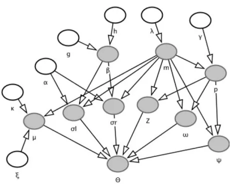
Finally, Figure2.1describes the dependencies between constants and variables involved in the

Bayesian network of RJMCMC mixture parameter learning, and then, a typical learning procedure of AGM can be summarized as follows:

Input:Data observationsX and component numberM

(1) Initialization

(2) Stept: Fort= 1, . . .

Gibbs sampling part

(a) GenerateZ(t)from Eq. (4)

(e) Compute acceptance ratiorfrom Eq. (13)

(f) Generateα=min[1, r]andu∼U_[0_,_1]

(g) Ifu≥αthenξ(t) =ξ(t−1)

RJMCMC part

(h) Generateu0 _∼_U

[0,1]. Ifbm>=u0, perform split or birth step, then calculate acceptance

probabilityA. If the step is accepted, setm=m+ 1.

(i) Generateu0 _∼_U

[0,1]. Ifdm >=u0, perform merge or death step, then calculate

(23)

Figure 2.1: DAG of RJMCMC parameter learning Bayesian network

2.3.1 Model Selection

Theoretically, RJMCMC learning process should always be able to derive the optimal

compo-nents numberM. However, because of the stochastic sampling, improper proposal distributions or

bad initialization parameters, learning result based on a single estimation run is not always satis-factory. In order to establish a robust parameter estimation algorithm, we evaluate the estimation outputs derived from multiple RJMCMC runs with different initial values of components number

by calculating their marginal likelihood with the Laplace approximation [10] on the logarithm scale

which is defined as follows:

log(p(X |M)) = log(p(X |Θˆ, M)) + log(π( ˆΘ|M)) + Np

2 log(2π) + 1

2log(|H( ˆΘ)|) (22)

whereΘˆ denotes the proposed optimal parameter set derived from a specific learning process and

π( ˆΘ|M) is the prior density of mixture parameters as well as its Hessian matrix H( ˆΘ) which is

(24)

Figure 2.2: Original synthetic data grouping and learning results

2.4 Experimental Results

2.4.1 Design of Experiments

Firstly, we apply the AGM model to both synthetic data and intrusion detection. For synthetic data validation, testing observations will be generated from AGM with known components number

M and experimental results will be evaluated by comparing the estimated and actual mixture

pa-rameters. In intrusion detection application, we select NSL-KDD dataset [31] as testing database.

K-means algorithm is used for initialization and the results analysis will be based on statistics de-rived from confusion matrix. Then, the proposed approach will be deployed to the Spambase spam filtering database contains multiple spam textual features including spam word/character dictionar-ies and profiles of uninterrupted capital letter sequences.

2.4.2 Synthetic Data

The main goals of this section are feasibility analysis and efficiency evaluation of the AGM

learning algorithm. The number of observations is set to 300 grouped into two clusters (M = 2).

Hyperparameters are set toγj = 1[32] for sampling mixture weightpj from Eq. (9). ηandτ are

considered asd-dimensional zero vectors in prior distributions of mixture parameterξ.

Different proposed component numbers (M0 _{= 1}_{, . . . ,}₅_{) are tested during the AGM learning}

process and the statistics are summarized in Table2.1. In order to select the best number of

com-ponents, we consider marginal likelihood as described in [10]. The probability density functions

(25)

Figure 2.3: (a) Original synthetic data grouping; (b) AGM clustering results

accepted moves for each component.

In terms of the best fit result, the accuracy is evaluated by calculating the Euclidean distance

between original and estimated mixture parameter setsξandξˆ(Table2.2). In summary, the

estima-tion of mean is accurate because the Euclidean distance betweenµjandµˆjis small but the distance

between standard deviationσlj, σrj andσˆlj,ˆσrj is slightly significant. However, this difference has

not affected the clustering result.

2.4.3 Intrusion Detection

Along with the rapid growth of information technologies, personal and commercial behaviors tend to rely on computer network and Internet environments. However, based on the character-istics of networking, exposing sensitive privacy and valuable business secret online is extremely

(26)

Table 2.1: AGM Learning Statistics Component numberM0 Moves accepted Acceptance ratio Marginal likelihood 1 22 7.33% -1596.143 2 11 3.67% -1500.370 3 14 4.67% -1684.518 4 63 21.00% -1522.148 5 39 13.00% -1517.533

Table 2.2: Accuracy Analysis (M0 ₌_M _{= 2}₎

Component numberj = 1 Mean (µj) Left standard deviation (σlj) Right standard deviation (σrj) ξ [-15.00, 0.00] [10.00, 1.00] [1.00, 1.00] ˆ ξ [-14.99, 0.25] [4.77, 1.13] [2.31, 1.88] Euclidean Distance 0.246 5.236 1.581 Component numberj = 2 Mean (µj) Left standard deviation (σlj) Right standard deviation (σrj) ξ [15.00, 0.00] [1.00, 1.00] [10.00, 1.00] ˆ ξ [14.02, -0.24] [2.04, 1.04] [5.70, 1.59] Euclidean Distance 1.010 1.036 4.338

(27)

traced, therefore, compromise network security. Cisco 2017 Annual Cybersecurity Report (ACR)

[33] pointed out a crucial fact that more than one-third of organizations that experienced a breach in

2016 reported more than 20 percent of customer, opportunity and revenue loss. As a consequence, more than 90 percent of these organizations are improving threat defense technologies and processes by enhancing IT and security functions, increasing security training of employees and implementing

risk mitigation techniques. Recently, machine learning-based intrusion detection solutions [34,35]

are drawing more attention because of their efficiency and flexibility.

Earlier intrusion prevention approaches, such as authentication, avoiding programming errors and encryption, were proven as insufficient because along with the increasing of the complexity of network-based software systems, exploitable weaknesses are inevitable due to programming issues. Moreover, authentication and encryption are not always reliable since credentials could be leaked and encryption algorithm could also be compromised by applying powerful hacking techniques to make the attack feasible. In consequence, once intrusion happens, detection will be harder than prevention and sometimes victims could not be even aware of it. Therefore, many supervised data mining solutions were proposed in terms of misuse and anomaly detection systems by establishing known intrusion scenarios, normal usage patterns and the sequential interrelations between user

op-erations to identify intrusion behaviors [36]. However, the disadvantages of supervised intrusion

detection systems are significant since predefined patterns and interrelations are inconsistent con-cerning the system upgrades and newly-founded intrusions which could lead to incessant intrusion detection system adjustment and affect its performance. Furthermore, inductive bias and overfitting problems caused by poor training datasets will also affect the accuracy of the systems. Therefore,

researchers are paying more attention to unsupervised solution [37,38] for seeking flexibility and

robustness.

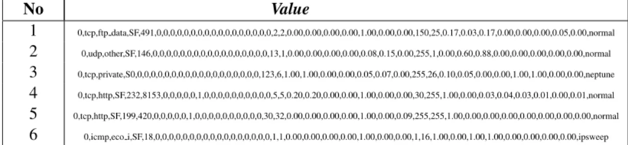
Therefore, we select NSL-KDD [31] (Table2.3), an improved KDDCUP’99 intrusion-detection

data-set, as the testing target since redundant records have been removed from original dataset to avoid potential learning bias. Before applying the testing models onto the dataset, the data pre-processing is needed since discrete enumerated values must be translated to numerical ones and be normalized properly to lead an accurate result. Therefore, we substitute enumerated values with their numbers of occurrences which could reflect the density distribution of discrete values. Having all numerical data in hand, we apply feature scaling method to normalize numerical values between

(28)

Table 2.3: Original NSL-KDD data records No Value 1 0,tcp,ftp data,SF,491,0,0,0,0,0,0,0,0,0,0,0,0,0,0,0,0,0,2,2,0.00,0.00,0.00,0.00,1.00,0.00,0.00,150,25,0.17,0.03,0.17,0.00,0.00,0.00,0.05,0.00,normal 2 0,udp,other,SF,146,0,0,0,0,0,0,0,0,0,0,0,0,0,0,0,0,0,13,1,0.00,0.00,0.00,0.00,0.08,0.15,0.00,255,1,0.00,0.60,0.88,0.00,0.00,0.00,0.00,0.00,normal 3 0,tcp,private,S0,0,0,0,0,0,0,0,0,0,0,0,0,0,0,0,0,0,0,123,6,1.00,1.00,0.00,0.00,0.05,0.07,0.00,255,26,0.10,0.05,0.00,0.00,1.00,1.00,0.00,0.00,neptune 4 0,tcp,http,SF,232,8153,0,0,0,0,0,1,0,0,0,0,0,0,0,0,0,0,5,5,0.20,0.20,0.00,0.00,1.00,0.00,0.00,30,255,1.00,0.00,0.03,0.04,0.03,0.01,0.00,0.01,normal 5 0,tcp,http,SF,199,420,0,0,0,0,0,1,0,0,0,0,0,0,0,0,0,0,30,32,0.00,0.00,0.00,0.00,1.00,0.00,0.09,255,255,1.00,0.00,0.00,0.00,0.00,0.00,0.00,0.00,normal 6 0,icmp,eco i,SF,18,0,0,0,0,0,0,0,0,0,0,0,0,0,0,0,0,0,1,1,0.00,0.00,0.00,0.00,1.00,0.00,0.00,1,16,1.00,0.00,1.00,1.00,0.00,0.00,0.00,0.00,ipsweep x0₌ x−min(x) max(x)−min(x) (23)

wherexandx0 _{denote original and normalized values. In this way we could use unified proposal}

distribution for every dimension with the same value of hyperparameter Σ during random walk

MCMC sampling step (Table2.4).

K-means clustering algorithm [39] is chosen for the comparison of accuracy. Testing data

records with total amount of 25192 (20% of NSL-KDD dataset) are clustered into two groups with

11743 intrusions and 13449 normal behaviors indicating components numberM0 _{= 2}_{. In order to}

better evaluate the pros and cons of models, results derived from Gaussian mixture model (GMM) will also be taken into consideration. The comparison based on confusion matrices resulted from

K-means, GMM and AGM model (Table2.5) reveals the fact that based on a less accurate initialization

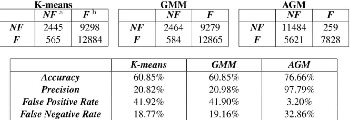
given by K-means (60.85%), GMM performs almost the same way as K-means and the difference between these two models is trivial. In contrast, AGM model makes a significant improvement with much higher accuracy rate (80.47%) and precision percentage (96.86%), while much lower false positive rate (4.26%) illustrating AGM model is capable of effectively detecting intrusions from background noises. Compared with K-means and GMM, AGM model has a higher false negative rate (28.58%) which means it tends to strictly identify normal behaviors as intrusions which could be mitigated by reducing dimensions of dataset using feature selection methodologies.

(29)

Table 2.4: Translation and Normalization of Internet Protocols (Enumerated Values) Internet Protocols Number of Occur-rences Normalized Values ICMP 1655 0 UDP 3011 0.071867 TCP 20526 1

Table 2.5: Confusion Matrices and Statistics of K-means, GMM and AGM Models

K-means NFa Fb NF 2445 9298 F 565 12884 GMM NF F NF 2464 9279 F 584 12865 AGM NF F NF 11484 259 F 5621 7828 K-means GMM AGM Accuracy 60.85% 60.85% 76.66% Precision 20.82% 20.98% 97.79%

False Positive Rate 41.92% 41.90% 3.20%

False Negative Rate 18.77% 19.16% 32.86%

(30)

Table 2.6: AGM Statistics Init. Comp. Numberm Accuracy Integrated Likelihood m= 1 55.64% 5.7074e5 m= 2 51.21% 4.0543e5 m= 3 58.99% 8.4238e5 2.4.4 Spam Filtering

Statistics reveal a crucial fact that more than 59% of worldwide e-mail traffic is considered

as unsolicited messages, also well known as spams, in 2017 [40]. Most spams are irritating and

resource-consuming, and some of them are extremely dangerous in terms of phishing scam, fee fraud, job offer scam, etc,. Since the damages of spam are persistent and significant not only for in-dividuals but also for governments, companies and organizations, many spam filtering technologies have been proposed to address this issue and eliminate unwanted e-mails automatically over recent decades.

Consequently, a well organized Spambase dataset [41] is selected with attributes related to

mul-tiple spam textual features including spam word/character dictionaries and profiles of uninterrupted capital letter sequences. Data pprocessing includes Scaling-based data normalization which re-scales numerical values within the range between 0 and 1 and label extraction for generating confu-sion matrix. To better evaluate the performance and accuracy of AGM model under different initial

number of components, the integrated likelihood [10] values are given in Table2.6 to identify the

best-fit result. Obviously, the result with initial component numberm= 3has the largest integrated

likelihood value (8.4238e5). Therefore, we select it as the best-fit result and make horizontal

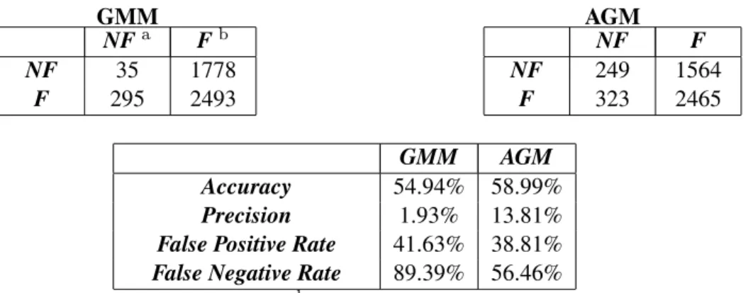
com-parison with GMM. Statistics in Table2.7reveal the fact that comparing to GMM, AGM provides

higher accuracy and precision, additionally, lower false positive rate and false negative rate indi-cate that AGM outperforms GMM. However, because of the nature of spambase, the performance of both mixture models is not satisfactory since most of spams cannot be identified. Therefore, data-based adjustment of the model might lead to a better result in the future.

(31)

Table 2.7: Confusion Matrices and Statistics of GMM and AGM GMM NFa Fb NF 35 1778 F 295 2493 AGM NF F NF 249 1564 F 323 2465 GMM AGM Accuracy 54.94% 58.99% Precision 1.93% 13.81%

False Positive Rate 41.63% 38.81%

False Negative Rate 89.39% 56.46%

a_{Non fault-prone,}b_Fault-prone.

2.4.5 Conclusion

This chapter firstly illustrated a new intrusion detection approach by applying asymmetric Gaus-sian mixtures with a fully BayeGaus-sian learning process which is achieved by applying a hybrid sampling-based MH-within-Gibbs learning algorithm. According to the experiment results, the AGM model is proved as an effective approach for clustering. In spite of the advantages of AGM we mentioned above, some improvements are still needed to promote the accuracy and flexibility and mitigate the drawbacks. Therefore, we shall extend the Bayesian learning process and introduce model selection and feature selection methodologies to improve the performance in the case of high-dimensional datasets.

(32)

Chapter 3

Unsupervised Learning with Feature

Selection: Application to Image

Categorization

3.1 Introduction

Recently, as the consequence of frequent usage of mobile phone, social media and cloud stor-age, digitalized visual data such as photos and pictures brings difficulties for management and anal-ysis. Unlike those within text-based documents, indexing and comparison among images could be challenging. Therefore, image categorization is becoming one of the most interesting research topics in computer vision community. Indeed, finding relevant images from a rapidly growing unannotated image database is challenging which makes the previous time-consuming manual cat-egorization methods infeasible. Automated methods such as machine-learning-based approaches

[42] introduce image representation methodologies for visual feature extraction and both generative

and discriminative classifiers for categorization. Meanwhile, modern machine-learning-based so-lutions can be divided into two main streams, classification-based supervised and clustering-based unsupervised ones. Compared to supervised solutions, unsupervised approach has no assumption on the number of groups, therefore, friendly to new added images and categories which makes it more suitable for increasing datasets. Moreover, it also immunizes against learning biases and overfitting problems that commonly exist in most supervised approaches if model training is inappropriate.

(33)

Consequently, unsupervised categorization of images or image parts [43,37,38] has an important role for image and video summarization, human action recognition, and image search etc,. It can also be seen as a pre-processing step for supervised methodologies for classification or

segmen-tation. As upgrade of single-mathematical-model-based methodologies, mixture models [6, 7,8]

can be seen as a superimposition of certain mixture components sharing dependencies with each other, therefore, lead to outstanding performance especially for high-dimensional and multi-cluster datasets.

Before deploying UIUC sports event database [44] to validate AGM framework, image

process-ing is needed because images should be represented as visual features and, eventually, be translated

into numerical data. As we discussed in Chapter2, parameter estimation could be challenging and

highly affects the performance of mixture models especially for high-dimensional data sets. For this

reason, we decided to adopt scale-invariant feature transform (SIFT) [45] to detect and describe

im-age features even under changes in imim-age scale, noise and illumination. However, generated SIFT features have to be categorized and features that belong to each image should be considered as

his-tograms to be the input of AGM model. Therefore, bag-of-visual-words [46] and probabilistic latent

semantic analysis (pLSA) [47] are responsible for the generation of features histogram. Meanwhile,

high-dimensionality will also bring difficulties to classifiers since previous approaches assume all the features of observations have the same weight of importance and carry pertinent information which is not always the case and many of those features can be irrelevant for clustering purpose. In order to tackle this problem and define relevance and importance of features, feature selection

tech-niques [4,23] should be taken into consideration. Eventually, irrelevant and unneeded information

will be filtered by feature selection.

3.2 Dimensionality Reduction for AGM

The AGM model defined in Eq. (2) assumes that all the dfeatures of observations have the

same weight of importance and carry pertinent information which is not always the case and many of those features can be irrelevant for clustering purpose. In order to tackle this problem and

de-fine relevance and importance of features, feature selection techniques [4,23] should be taken into

(34)

Gaussian distribution, respectively. Then, Eq. (2) can be reformulated with the feature relevancy

approach suggested in [22] as follows:

p(X |Θ,Ψ,Φ) = N Y i=1 M X j=1 pj d Y k=1 p(Xik|ξjk)φkN(Xik|ψk)1−φk (24)

whereN(Xik|ψk)denotes the likelihood thatk-th feature ofi-th observation is irrelevant where

ψk = (µ0_k, σ0_k) is the parameters set of background Gaussian distribution. Φ = (φ1, . . . , φd) is a

binary relevancy vector whereφk = 1ifk-th feature is relevant orφk = 0otherwise. If we consider

the relevancy vector Φas a latent variable, the complete likelihood function of AGM model with

full parameter set will be given as follows:

p(X |Θ0_{) =} N Y i=1 M X j=1 pj d Y k=1 [ωkp(Xik|ξjk) + (1−ωk)N(Xik|ψk)] (25) where Θ0 _{= (Θ}_,_Ψ_,_Ω) _and _{Ω = (}_ω

1, . . . , ωd) is the relevancy weight with value range of

0≤ωd≤1which represents the probability thatk-th feature is relevant. Finally, the calculation of

relevancy weightωkis given as follows:

ωk= QN i=1PMj=1pjp(Xik|ξjk) QN i=1 PM j=1pjp(Xik|ξjk) +QNi=1N(Xik|ψk) (26)

Therefore, irrelevant features only have small contribution for the clustering process, thus the us-ability of AGM model is extended to more common and complicated cases such as high-dimensional noisy applications. The parameter learning algorithm with feature selection can be described as fol-lows:

Input:Data observationsX and component numberM

(1) Initialization

(2) Stept: Fort= 1, . . .

(35)

(a) GenerateZ(t)from Eq. (6) and (25)

(e) Calculate relevancy weightω_k(t)from Eq. (26)

(f) Generate background Gaussian parametersψ_k(t)by random walk

(g) Compute acceptance ratiorfrom Eq. (13)

(h) Generateα=min[1, r]andu∼U_[0_,_1]

(i) Ifu≥αthenξ(t) =ξ(t−1)_{, ψ}(t) k =ψ (t−1) k , ω (t) k =ω (t−1) k RJMCMC part (j) Generateu0 _∼_U

[0,1]. Ifbm>=u0, perform split or birth step, then calculate acceptance

probabilityA. If the step is accepted, setm=m+ 1.

(k) Generateu0 _∼_U

[0,1]. Ifdm >=u0, perform merge or death step, then calculate

accep-tance probabilityA0_{. If the step is accepted, set}_m₌_m₋₁_.

Figure3.1illustrates updated DAG parameter dependency figure with feature selection related

parameters added.

3.3 Image Categorization

A challenging UIUC sports event database [44] is selected for our target application which has

been evaluated by previous researches [48,43]. It has 1579 images in total and consists of 8 sports

event categories: rowing (250 images), badminton (200 images), polo (182 images), bocce (137 images), snowboarding (190 images), croquet (236 images), sailing (190 images), and rock climbing (194 images). The first step of image pre-processing is applying scale-invariant feature transform

(SIFT) on the original image files using difference of Gaussian (DoG) [45] (Figure3.2) as interest

point detector and then, visual feature will be translated into 128-dimensional feature descriptor

(36)

Figure 3.1: DAG of AGM Bayesian learning network with feature selection

image will be represented by a frequency histogram of occurrence of visual words inW. Since the

vocabulary size in our test is between 200 to 1000, we also adopted probabilistic latent semantic analysis (pLSA) to describe each image as several latent topics (aspect) and therefore, reduce the dimension of image representation. Before applying AGM model for clustering, normalization based on feature scaling method is added to restrain the range of numerical attributes which will improve the Bayesian learning performance. Finally, we deploy the proposed AGM model as an unsupervised classifier to categorize the whole database. The proposed model is tested against image representation generated with different vocabulary sizes between 200 to 1000 with an interval of 100 and latent aspect number between 15 to 50 with an interval of 5 in order to identify the best accuracy.

According to a comparison between K-means, Gaussian mixture model (GMM) and proposed AGM model reveals the fact that applying AGM to the sports event database leads to a significant clustering accuracy boost due to the best accuracy numbers of all the 3 classifiers illustrated in figure

3.3(a) (K-means: 22.17%, GMM: 29.26% and AGM: 46.04%). Moreover, the impact of accuracy

from different latent aspect numbers can be found in figure3.3(b). Finally, the detailed clustering

confusion matrix of AGM under the optimal vocabulary size (1000) and latent aspect number (30)

(37)

(38)

Figure 3.4: Confusion matrix of AGM model (Vocabulary size is 1000 and latent aspect number is 30)

adjustments and improvements to tackle high-dimensional datasets to achieve higher clustering ac-curacy.

(39)

Chapter 4

Conclusion

Our work is based on asymmetric Gaussian mixture (AGM) model and reversible jump Markov chain Monte Carlo (RJMCMC) learning algorithm. Previous efforts reveal the fact that AGM out-performs classic Gaussian mixture model (GMM) by taking asymmetric datasets into consideration which provides more flexibility. Our RJMCMC implementation is based on a hybrid sampling-based approach which takes advantages of both Metropolis-Hastings (MH) and Gibbs sampling methods, therefore, simplifies mathematical complexity and extends adaptability of the model. Moreover, without giving a fixed components number in advance, RJMCMC applies a dynamic data-based strategy to identify the optimal components number throughout iterations which makes the model learning a self-adaptive process. Since the model is nondeterministic, Laplace approx-imation based marginal likelihood is calculated for multiple runs as model selection procedure to improve the correctness and fitting accuracy. Moreover, the proposed AGM model includes fea-ture selection which can not only filters irrelevant and unneeded feafea-tures but also weights relevant features based on the pertinent information they carry.

In order to validate the performance and accuracy of the proposed approach, applications in-cluding intrusion detection, spam filtering and image categorization have been conducted and the results are analyzed and compared with popular machine learning models. Future research direc-tions will focus on model adjustments and improvements to tackle high-dimensional datasets and achieve high clustering accuracy. The proposed work could be applied to other applications such as

(40)

Bibliography

[1] N. Bouguila, D. Ziou, and E. Monga, “Practical bayesian estimation of a finite beta mixture

through gibbs sampling and its applications,” Statistics and Computing, vol. 16, no. 2, pp.

215–225, 2006.

[2] T. Elguebaly and N. Bouguila, “Background subtraction using finite mixtures of asymmetric

gaussian distributions and shadow detection,”Mach. Vis. Appl., vol. 25, no. 5, pp. 1145–1162,

2014.

[3] S. Richardson and P. J. Green, “On bayesian analysis of mixtures with an unknown number of

components (with discussion),”Journal of the Royal Statistical Society: series B (statistical

methodology), vol. 59, no. 4, pp. 731–792, 1997.

[4] T. Elguebaly and N. Bouguila, “Simultaneous bayesian clustering and feature selection

us-ing rjmcmc-based learnus-ing of finite generalized dirichlet mixture models,”Signal Processing,

vol. 93, no. 6, pp. 1531–1546, 2013.

[5] ——, “Bayesian learning of finite generalized gaussian mixture models on images,” Signal

Processing, vol. 91, no. 4, pp. 801–820, 2011.

[6] J. Yang, X. Liao, X. Yuan, P. Llull, D. J. Brady, G. Sapiro, and L. Carin, “Compressive

sens-ing by learnsens-ing a gaussian mixture model from measurements,”IEEE Transactions on Image

Processing, vol. 24, no. 1, pp. 106–119, Jan 2015.

[7] C. K. Wen, S. Jin, K. K. Wong, J. C. Chen, and P. Ting, “Channel estimation for massive mimo

using gaussian-mixture bayesian learning,”IEEE Transactions on Wireless Communications,

(41)

[8] N. Bouguila, “Count data modeling and classification using finite mixtures of distributions,”

IEEE Trans. Neural Networks, vol. 22, no. 2, pp. 186–198, 2011.

[9] A. P. Dempster, N. M. Laird, and D. B. Rubin, “Maximum likelihood from incomplete data

via the em algorithm,” Journal of the royal statistical society. Series B (methodological), pp.

1–38, 1977.

[10] N. Bouguila, D. Ziou, and R. I. Hammoud, “On bayesian analysis of a finite generalized

dirichlet mixture via a metropolis-within-gibbs sampling,”Pattern Anal. Appl., vol. 12, no. 2,

pp. 151–166, 2009.

[11] N. Bouguila and T. Elguebaly, “A fully bayesian model based on reversible jump MCMC and

finite beta mixtures for clustering,”Expert Syst. Appl., vol. 39, no. 5, pp. 5946–5959, 2012.

[12] S. Bourouis, M. A. Mashrgy, and N. Bouguila, “Bayesian learning of finite generalized

in-verted dirichlet mixtures: Application to object classification and forgery detection,” Expert

Syst. Appl., vol. 41, no. 5, pp. 2329–2336, 2014.

[13] W. K. Hastings, “Monte carlo sampling methods using markov chains and their applications,”

Biometrika, vol. 57, no. 1, pp. 97–109, 1970.

[14] S. Geman and D. Geman, “Stochastic relaxation, gibbs distributions, and the bayesian

restora-tion of images,” inReadings in Computer Vision. Elsevier, 1987, pp. 564–584.

[15] N. Bouguila, D. Ziou, and S. Boutemedjet, “Simultaneous non-gaussian data clustering,

fea-ture selection and outliers rejection,” inPattern Recognition and Machine Intelligence - 4th

International Conference, PReMI 2011, Moscow, Russia, June 27 - July 1, 2011. Proceedings, ser. Lecture Notes in Computer Science, S. O. Kuznetsov, D. P. Mandal, M. K. Kundu, and

S. K. Pal, Eds., vol. 6744. Springer, 2011, pp. 364–369.

[16] S. Boutemedjet, N. Bouguila, and D. Ziou, “A hybrid feature extraction selection approach

for high-dimensional non-gaussian data clustering,”IEEE Trans. Pattern Anal. Mach. Intell.,

vol. 31, no. 8, pp. 1429–1443, 2009.

[17] S. Raudys and A. K. Jain, “Small sample size effects in statistical pattern recognition:

(42)

[18] R. Kohavi and G. H. John, “Wrappers for feature subset selection,”Artif. Intell., vol. 97, no. 1-2, pp. 273–324, 1997.

[19] K. Z. Mao, “Identifying critical variables of principal components for unsupervised feature

selection,” IEEE Trans. Systems, Man, and Cybernetics, Part B, vol. 35, no. 2, pp. 339–344,

2005.

[20] C. Tsai and C. Chiu, “Developing a feature weight self-adjustment mechanism for a k-means

clustering algorithm,” Computational Statistics & Data Analysis, vol. 52, no. 10, pp. 4658–

4672, 2008.

[21] J. G. Dy and C. E. Brodley, “Feature selection for unsupervised learning,”Journal of Machine

Learning Research, vol. 5, pp. 845–889, 2004.

[22] M. H. Law, M. A. Figueiredo, and A. K. Jain, “Simultaneous feature selection and

cluster-ing uscluster-ing mixture models,”IEEE transactions on pattern analysis and machine intelligence,

vol. 26, no. 9, pp. 1154–1166, 2004.

[23] T. Elguebaly and N. Bouguila, “Simultaneous high-dimensional clustering and feature

selec-tion using asymmetric gaussian mixture models,”Image and Vision Computing, vol. 34, pp.

27–41, 2015.

[24] S. Fu and N. Bouguila, “Bayesian learning of finite asymmetric gaussian mixtures,” in

Pro-ceedings of The 31st International Conference on Industrial, Engineering & Other Applica-tions of Applied Intelligent Systems Montreal, QC, CA, June 25-28, 2018, 2018.

[25] ——, “Asymmetric gaussian mixtures with reversible jump MCMC,” in2018 IEEE Canadian

Conference on Electrical & Computer Engineering (CCECE) (CCECE 2018), Quebec City, Canada, May 2018.

[26] ——, “A bayesian intrusion detection framework,” inCyber Science 2018, Glasgow, Scotland,

UK, June 11-12, 2018, 2018.

[27] N. Bouguila and D. Ziou, “A powreful finite mixture model based on the generalized dirichlet

distribution: Unsupervised learning and applications,” in 17th International Conference on

Pattern Recognition, ICPR 2004, Cambridge, UK, August 23-26, 2004. IEEE Computer Society, 2004, pp. 280–283.

(43)

[28] ——, “Dirichlet-based probability model applied to human skin detection [image skin

detec-tion],” in2004 IEEE International Conference on Acoustics, Speech, and Signal Processing,

ICASSP 2004, Montreal, Quebec, Canada, May 17-21, 2004. IEEE, 2004, pp. 521–524. [29] D. Luengo and L. Martino, “Fully adaptive gaussian mixture metropolis-hastings algorithm,”

inIEEE International Conference on Acoustics, Speech and Signal Processing, ICASSP 2013, Vancouver, BC, Canada, May 26-31, 2013. IEEE, 2013, pp. 6148–6152.

[30] G. Casella, C. P. Robert, and M. T. Wells, “Mixture models, latent variables and partitioned

importance sampling,”Statistical Methodology, vol. 1, no. 1-2, pp. 1–18, 2004.

[31] M. Tavallaee, E. Bagheri, W. Lu, and A. A. Ghorbani, “A detailed analysis of the KDD CUP

99 data set,” in2009 IEEE Symposium on Computational Intelligence for Security and Defense

Applications, CISDA 2009, Ottawa, Canada, July 8-10, 2009. IEEE, 2009, pp. 1–6.

[32] M. Stephens, “Bayesian analysis of mixture models with an unknown number of

components-an alternative to reversible jump methods,”Annals of statistics, pp. 40–74, 2000.

[33] Investor.cisco.com. (2018) Cisco 2017 annual cybersecurity report. [Online].

Avail-able: https://investor.cisco.com/investor-relations/news-and-events/news/news-details/2017/

Cisco-2017-Annual-Cybersecurity-Report-Chief-Security-Officers-Reveal-True-Cost-of-Breaches-And-The-Ac default.aspx

[34] A. L. Buczak and E. Guven, “A survey of data mining and machine learning methods for

cyber security intrusion detection,” IEEE Communications Surveys Tutorials, vol. 18, no. 2,

pp. 1153–1176, Secondquarter 2016.

[35] R. A. R. Ashfaq, X.-Z. Wang, J. Z. Huang, H. Abbas, and Y.-L. He, “Fuzziness based

semi-supervised learning approach for intrusion detection system,”Information Sciences, vol. 378,

pp. 484 – 497, 2017.

[36] W. Lee and S. J. Stolfo, “Data mining approaches for intrusion detection,” in Proceedings

of the 7th USENIX Security Symposium, San Antonio, TX, USA, January 26-29, 1998, A. D.

Rubin, Ed. USENIX Association, 1998.

(44)

mix-[38] M. Azam and N. Bouguila, “Unsupervised keyword spotting using bounded generalized

gaus-sian mixture model with ICA,” in 2015 IEEE Global Conference on Signal and Information

Processing, GlobalSIP 2015, Orlando, FL, USA, December 14-16, 2015. IEEE, 2015, pp. 1150–1154.

[39] J. A. Hartigan and M. A. Wong, “Algorithm as 136: A k-means clustering algorithm,”Journal

of the Royal Statistical Society. Series C (Applied Statistics), vol. 28, no. 1, pp. 100–108, 1979.

[40] K. Lab. (2018) Spam: share of global email traffic 2014-2017. [Online]. Available:

https://www.statista.com/statistics/420391/spam-email-traffic-share/

[41] G. F. J. S. Mark Hopkins, Erik Reeber. (2018) Uci machine learning repository: Spambase

data set. [Online]. Available:http://archive.ics.uci.edu/ml/datasets/Spambase?ref=datanews.io

[42] Y. Han and X. Qi, “Machine-learning-based image categorization,” inInternational

Confer-ence Image Analysis and Recognition. Springer, 2005, pp. 585–592.

[43] W. Fan and N. Bouguila, “Infinite dirichlet mixture model and its application via variational

bayes,” inMachine Learning and Applications and Workshops (ICMLA), 2011 10th

Interna-tional Conference on, vol. 1. IEEE, 2011, pp. 129–132.

[44] L.-J. Li and L. Fei-Fei, “What, where and who? classifying events by scene and object recog-nition,” 2007.

[45] D. G. Lowe, “Object recognition from local scale-invariant features,” in Computer vision,

1999. The proceedings of the seventh IEEE international conference on, vol. 2. Ieee, 1999, pp. 1150–1157.

[46] L. Fei-Fei and P. Perona, “A bayesian hierarchical model for learning natural scene categories,” inComputer Vision and Pattern Recognition, 2005. CVPR 2005. IEEE Computer Society Con-ference on, vol. 2. IEEE, 2005, pp. 524–531.

[47] T. Hofmann, “Unsupervised learning by probabilistic latent semantic analysis,” Machine

learning, vol. 42, no. 1-2, pp. 177–196, 2001.

[48] F. Najar, S. Bourouis, A. Zaguia, N. Bouguila, and S. Belghith, “Unsupervised human action categorization using a riemannian averaged fixed-point learning of multivariate ggmm,” in

(45)

[49] G. Csurka, C. Dance, L. Fan, J. Willamowski, and C. Bray, “Visual categorization with bags

of keypoints,” inWorkshop on statistical learning in computer vision, ECCV, vol. 1, no. 1-22.

Prague, 2004, pp. 1–2.

[50] N. Bouguila, “Spatial color image databases summarization,” inProceedings of the IEEE

In-ternational Conference on Acoustics, Speech, and Signal Processing, ICASSP 2007, Honolulu, Hawaii, USA, April 15-20, 2007. IEEE, 2007, pp. 953–956.

[51] N. Bouguila and D. Ziou, “Improving content based image retrieval systems using finite

multi-nomial dirichlet mixture,” inMachine Learning for Signal Processing, 2004. Proceedings of

the 2004 14th IEEE Signal Processing Society Workshop. IEEE, 2004, pp. 23–32.

[52] S. Boutemedjet, D. Ziou, and N. Bouguila, “Unsupervised feature selection for accurate

rec-ommendation of high-dimensional image data,” inAdvances in Neural Information

Process-ing Systems 20, ProceedProcess-ings of the Twenty-First Annual Conference on Neural Information Processing Systems, Vancouver, British Columbia, Canada, December 3-6, 2007, J. C. Platt,