Bayesian estimation of P[Y \u3c X] Based on Record Values from the Lomax Distribution and MCMC Technique

Volume 15 | Issue 1 Article 25

5-1-2016

Bayesian estimation of P[Y < X] Based on Record

Values from the Lomax Distribution and MCMC

Technique

Mohamed A. W Mahmoud

Al-Azhar University, Cairo, Egypt

Rashad M. El-Sagheer

Al-Azhar University, [email protected]

Ahmed A. Soliman

Islamic University of Madinah, Medina, Saudi Arabia

Ahmed H. Abd Ellah

Sohag University, Sohag, Egypt

Follow this and additional works at:http://digitalcommons.wayne.edu/jmasm

Part of theApplied Statistics Commons,Social and Behavioral Sciences Commons, and the Statistical Theory Commons

Recommended Citation

Mahmoud, Mohamed A. W; El-Sagheer, Rashad M.; Soliman, Ahmed A.; and Abd Ellah, Ahmed H. (2016) "Bayesian estimation of P[Y < X] Based on Record Values from the Lomax Distribution and MCMC Technique,"Journal of Modern Applied Statistical Methods: Vol. 15 : Iss. 1 , Article 25.

Cover Page Footnote

Mohamad Mahmoud is Faculty of Science in the Mathematics Department. Dr. Rashad Mohamed El-Sagheer is a lecturer of Mathematical Statistics in the Mathematics Department, Faculty of Science. Email at [email protected],

Bayesian Estimation of P[Y<X] Based on

Record Values from the Lomax Distribution

and MCMC Technique

Mohamed A. W. Mahmoud Al-Azhar University Cairo, Egypt Rashad M. El-Sagheer Al-Azhar University Cairo, Egypt Ahmed A. Soliman Islamic University of Madinah Medina, Saudi Arabia

Ahmed H. Abd Ellah Sohag University

Sohag, Egypt

Our interest is in estimating the stress-strength reliability R = P[Y < X], where X and Y follow the Lomax distribution with common scale parameter. We discuss the problem in the situation where the stress measurements and the strength measurements are both in terms of records. Firstly, we obtain the MLE of R in general case (the common scale parameter is unknown). The MLE of the three unknown parameters can be obtained by solving one non-linear equation. We provide a simple fixed point type algorithm to find the MLE. We propose percentile bootstrap confidence intervals of R. A Bayes point estimator of R, and the corresponding credible interval using the MCMC sampling technique have been proposed. Secondly, assuming the common scale parameter is known, the MLE of R is obtained. Using exact distributions of the MLEs of the two unknown parameters, we construct the exact confidence interval of R. In this case, Bayes estimators have been obtained using Lindley's approximations. Analysis of a simulated data set has been presented for illustrative purposes. Finally, the different proposed methods have been compared via Monte Carlo simulation study.

Keywords: Stress-strength model, Lomax distribution, maximum likelihood estimation, bootstrap confidence intervals, credible intervals, Gibbs sampling, Markov chain Monte Carlo

Introduction

The problem of estimating R = P[Y < X] arises in the context of mechanical reliability of a system with strength (or supply) X and stress (or demand) Y, and R

is chosen as a measure of system reliability. The system fails if and only if at any time the applied stress is greater than its strength. This type of reliability model is known as the stress-strength model. This problem also arises in situations where X

and Y represent lifetimes of two devices and one wants to estimate the probability that one fails before the other. For example, in biometrical studies, the random variable X may represent the remaining lifetime of a patient treated with a certain drug, and Y represent the remaining lifetime when treated by another drug.

Review of literature

Parametric and nonparametric inferences on R for several specific distributions of

X and Y under different conditions have been found in the literature. Nadarajah (2004a; 2004b) estimated R = P[Y < X] from Logistic and Laplace distributions. Kundu and Gupta (2005) derived the maximum likelihood estimator of R and its asymptotic distribution when X and Y are independently distributed as generalized exponential distribution. Surles and Padgett (2001) considered the estimation of R where X and Y are Burr-X random variables. The theoretical and practical results on the theory and applications of the stress-strength relationships in industrial and economic systems during the last decades are collected and digested in Kotz, Lumelskii, and Pensky (2003).

The class of life-time distributions (in particular, exponential and gamma) is considered by Nadarajah (2003). Estimation of R from exponential case with common location parameter (Baklizi & El-Masri, 2004), Burr-III (Mokhlis, 2005), beta (Nadarajah, 2005a), gamma (Nadarajah, 2005b), bivariate exponential (Nadarajah & Kotz, 2006), and Weibull (Kundu & Gupta, 2006) distributions were also studied. Inferences on reliability in two-parameter exponential stress-strength model (Krishnamoorthy, Mukherjee, & Guo, 2007) and ML estimation of system reliability for Gompertz distribution (Saraçoglu & Kaya, 2007) were considered. Kakade, Shirke, and Kundu (2008) studied the exponentiated Gumbel case. Baklizi (2008a; 2008b) studied some inference problems of estimating R based on record values. Kundu and Raqab (2009) considered the estimation of R when X and Y are independent and both having three parameter Weibull distribution with common shape and location parameters, but different scale parameters.

inference for the Burr type XII distribution based on records. Lomax (1954) used this distribution in the analysis of business failure data. Balkema and De Haan (1974) showed that this distribution arises as a limit distribution of residual lifetime at great age. The Lomax distribution includes increasing and decreasing hazard rates as well, and was shown to be useful for modeling and analyzing the life time data in medical and biological sciences and engineering, etc.

Many statistical methods have been developed for this distribution. For a review of the Lomax distribution, see Habibullah and Ahsanullah (2000), Upadhyay and Peshwani (2003), and Abd Ellah (2003; 2006) and references therein. A great deal of research was done on estimating the parameters of a Lomax distribution using both classical and Bayesian techniques. The form of the probability density function (pdf) and cumulative distribution function (cdf) with the scale parameter λ and the shape parameter α of the Lomax distribution, denoted by Lomax(λ, α), are given, respectively, by

 





 1

f x  x   , x0,  , 0 (1)

 





F x  1  x , x0,  , 0 (2) Record data arise in a wide variety of practical situations. Examples include industrial stress testing, meteorological analysis, hydrology, seismology, sporting, athletic events, and oil and mining surveys. Specifically, Let {Xj, j ≥ 1}be a sequence of independent identically continuous random variables. An observation

Xj will be called an upper record value if its value exceeds that of all previous observations. That is, Xj is an upper record if Xj > Xi for every i < j. An analogous definition can be given for lower record values. Record values can be viewed as order statistics from a sample whose size is determined by the values and the order of occurrence of the observations.

Maximum Likelihood Estimator of R

Suppose that X is the strength of a component which is subject to stress Y. The system fails if and only if, at any time, the applied stress is greater than strength. Let X be a random variable whose pdf is a Lomax distribution with parameters λ and α, denoted by Lomax(λ, α), and Y is another Lomax distribution random





₀



 



P P | P R Y X Y X X x X x dx



 

        



(3)

The interest is in estimating R when the data available on both X and Y are in the form of upper record values. To compute the MLE of R, compute the MLE of α and

β. Suppose x = xU(1), xU(2),…, xU(n) is the first upper record values of size n from

Lomax(λ, α), and y = yU(1), yU(2),…, yU(m) is an independent set of the first upper

record values of size m from Lomax(λ, β). The likelihood functions for both observed records x and y are given, respectively, by





 

_{ }

 

   

 

1 U 1 U 1 U f L , | f 1 F n i n i i x x x      



x (4) and





 

_{ }

 

   

 

1 U 2 U 1 _U g L , | g 1 G m j m j _j x y x      



y , (5)

where f and F are the pdf and cdf of X ∼ Lomax(λ, α), respectively, and g and G are the pdf and cdf of Y ∼ Lomax(λ, β), respectively (Arnold, Balakrishnan, & Nagaraja, 1998). Substituting f, F, g and G in the likelihood functions,











_{ }



1 1 U L  , |x  n  x, exp_ln x _n  _ (6)











_{ }



2 2 U L , | m , exp ln m y    y    y  _  _ , (7) where







_{ }



1







_{ }



1 1 U 2 U 1 1 , , , n m i j i j x y











    x 



  y 



 . (8)

Therefore, the joint Log-likelihood function of the observed records x and y under Lomax distribution is











 



 







 





 



U U U U 1 1 , , | data ln ln ln ln ln ln ln n n m m i j i j n m x y x y                         



 



 (9)

The MLEs of λ, α, and β, say



ˆ,



ˆ, and ˆ, respectively, can be obtained as the solution of     1   1   U U U U ˆ ˆ ˆ ˆ 1 1 0 ˆ ˆ ˆ ˆ ˆ n m i j n m i j x y x y             _{    }  







 (10)  



U ˆ



ˆ ln ln 0 ˆ n n x







    (11)  



U ˆ



ˆ ln ln 0 ˆ m m y        . (12) From (11) and (12),   1 U ˆ n ln x _ˆn 1





       _ _        (13)   1 U ˆ _{ln 1} ˆ m y m





       _ _        , (14)

 

                1 1 U U 1 1 U U 1 _U 1 _U f ln 1 ln 1 ln 1 ln 1 1 1 n m U n U m n m n m i _i j _j x y n m x y n m x y x y                          _ _   _  _                   _  _   _  _  _{  }  _{  }    





(15)

Therefore,



ˆ can be obtained as the solution of the non-linear equation of the form

 

h   (16) where

 

                1 1 1 U U U U 1 1 U 1 1 U U U h ln 1 ln 1 ln 1 1 1 ln 1 n m n n n m m i j m i j x y _n x n m x y m y x y



















        _{     }   _{  }    _  _  _   _  _ _{ }  _  _                        _  _  _  _  _  _{ }     





_

Since



ˆ is a fixed point solution of non-linear equation (15) and, therefore, it can be obtained by using a simple iterative scheme as follows:

 

1

h _j _j , (17)

where λj is the jth _{iterate of}



ˆ_{. The iteration procedure should be stopped when}

1

j j

  is sufficiently small. Therefore, the MLE of R becomes

ˆ ˆ ˆ _ˆ R      (18)

Bootstrap Confidence Intervals

Confidence intervals are proposed based on the parametric bootstrap methods (i) percentile bootstrap method (Boot-p) based on the idea of Efron (1982) and (ii) bootstrap-t method (Boot-t) based on the idea of Hall (1988). The algorithms for estimating the confidence intervals of R using both methods are illustrated as follows:

Percentile Bootstrap Method

1. From the original two samples of upper records {xU(1), xU(2),…, xU(n)} and

{yU(1), yU(2),…, yU(m)}, compute ML estimates



ˆ,



ˆ, ˆ , and Rˆ

2. Using



ˆ and



ˆ , generate a bootstrap upper record sample

     



* * *



U 1, U 2, , Un

x x x and, similarly, using



ˆ and ˆ, generate a bootstrap upper record sample



y_{U 1}*_{ },y_{U 2}*_{ }, ,x*_{U m}



. Based on these data, we compute the bootstrap estimates, say



ˆ*,



ˆ*, ˆ*, and Rˆ*

3. Repeat step 2 Nboot times

4. Let V

 

x P



Rˆ*x



be the cdf of Rˆ*. Define Rˆ_boot V1

 

x for a given

x. The approximate 100(1 – γ)% confidence interval of R is given by

Boot-p Boot-p ˆ _, ˆ ₁ 2 2 R



R



    _       _{   }   . (19) Bootstrap-t Method

1. From the original two samples of upper records {xU(1), xU(2),…, xU(n)} and

{yU(1), yU(2),…, yU(m)}, compute ML estimates



ˆ,



ˆ, ˆ , and Rˆ

2. Using



ˆ and



ˆ , generate a bootstrap upper record sample

     



* * *



U 1, U 2, , Un

x x x and, similarly, using



ˆ and ˆ, generate a bootstrap upper record sample



y_{U 1}*_{ },y_{U 2}*_{ }, ,x*_{U m}



. Based on these data, we compute the bootstrap estimates, say



ˆ* ,



ˆ* , ˆ* , and compute the bootstrap estimate of R using (18), Rˆ*, and following statistic:





 

* * * ˆ ˆ ˆ Var n R R T R   ,

where Var

 

Rˆ* is obtained using the Delta method (Greene, 2000) 3. Repeat step 2 N boot times

4. For the T*_{values obtained in step 2, determine the upper and lower bounds}

of the 100(1 – γ)% confidence interval of R as follows: let H(x) = P(T* _{≤ x)}

be the cdf of T*_{. For a given x, define}

 

1

 

₁

 

2 Boot-t

ˆ ˆ _Var ˆ _H

R x  R n R  x .

Here also, Var

 

Rˆ can be computed as same as computing the Var

 

Rˆ* . The approximate 100(1 – γ)% confidence interval of R is given by

Boot-t Boot-t ˆ _, ˆ ₁ 2 2 R



R



    _       _{   }   (20)

Bayes Estimation of R Using MCMC

The advantage of MCMC is that it not only gives a point estimate of the parameter, but also gives an interval estimation based on the final simulated empirical distribution. MCMC is essentially an iterative sampling algorithm, drawing values from the posterior distributions of the parameter in the concerned model. Consider the MCMC method to generate samples from the posterior distributions and then compute the Bayes estimates of R under upper record values from Lomax distribution. A wide variety of MCMC schemes are available. An important sub-class of MCMC methods are Gibbs sampling and more general Metropolis-Hastings (M-H) algorithm (Metropolis, Rosenbluth, Rosenbluth, Teller, & Teller, 1953; Hastings, 1970). For more details about MCMC and the related methodologies, one can refer to Gentle (1998), Chen, Shao, and Ibrahim (2000), and Robert and Casella (2004).

Now, obtain the Bayes estimation of R under assumption that the parameters (λ, α, β) are independent random variables. The Bayes estimate of R under the squared error loss and the corresponding credible interval by the Gibbs sampling

technique are considering. It is assumed that (λ, α, β) have independent gamma priors with the pdf's





 





1 1 1 1 1 1 1 1 1 exp , 0 | , 0, 0 a a b b a a b            _{ }  _  (21)





 





2 2 1 2 2 2 2 2 2 exp , 0 | , 0, 0 a a b b a a b            _{ }  _  (22)





 





3 3 1 3 3 3 3 3 3 exp , 0 | , 0, 0 a a b b a a b            _{ }  _  (23)

where, a1, b1, a2, b2, a3, and b3 are chosen to reflect prior knowledge about λ, α, and

β. The expression for the posterior can be obtained up to proportionality by multiplying the likelihood with the prior and this can be written as





     

_

_{ }

_

_

_

 









 









3 1 1 2 1 1 * 1 2 1 2 U 3 , , | data , , exp exp ln exp ln m a a n a n U m b b x b y  

  





















               _   _      _   _   x y (24)

where η1(x, λ), η2(y, λ) are given in (8) and





   







 





 







1 1 * 1 U 1 2 1 | , , data , , exp a n U m x y b                        x  y  (25)





U  * 2 | , data Gamma 2, 2 ln 1 n x n a b

 



    _   _  __     (26)





U  * 3 | , data Gamma 3, 3 ln 1 m x m a b

 



    _   _  __     . (27)

It can be seen that (26) is a gamma density with shape parameters (n + a2) and

  U 2 ln 1 n x b



      _ _  _{ }

  and (27) is a gamma density with shape parameters (m + a2)

and b₃ ln yU m 1



      _ _  _{ }

 . Therefore, samples of α and β can be easily generated

using any gamma generating routine. However, in our case, the conditional posterior distribution of λ equation (25) cannot be reduced analytically to well-known distributions and, therefore, it is not possible to sample directly by standard methods. However, the plot of it shows that it is similar to a normal distribution. To generate random numbers from this distribution, use the Metropolis-Hastings method with normal proposal distribution.

Therefore, the algorithm of Gibbs sampling is as follows:

 Start with an





 0 



ˆ



and set = 1

 Generate α(t) _from U  2 2 Gamma n a b, ln x n 1



       _ _  _{ }    Generate β(t) _from U  3 3 Gamma n a b, ln y m 1



       _ _  _{ }  

 Using Metropolis-Hastings (see Metropolis et al., 1953), generate λ(t) _from

(25) with the N(λ(t – 1)_{, σ}2_{) proposal distribution, where σ}2 _is

variance-covariance matrix

 Compute λ(t)_{, α}(t)_{, and β}(t)_{. Then compute}  

      t t t t R







   Set t = t + 1

 Repeat steps 2-5 N times





  1 1 E | data N i i M R R N M    



, (28)

where M is the burn-in period (that is, a number of iterations before the stationary distribution is achieved) and posterior variance of R becomes







 

_

_



2 1 1 ˆ ˆ V | data = E | data N i i M R R R N M    



(29)

 To compute the credible intervals of R, usually, take the quintiles of the sample as the end points of the interval. Order R(M + 1)_{, R}(M + 2)_{,…, R}(N) _{as R}(1)_,

R(2)_{,…, R}(N – M)_{. Then the 100(1 – γ)% symmetric credible interval is}

  1   2 2 , N M N M R_{ } R_{  }                      (30)

Estimation of R if

λ is Known

Consider the estimation of R and the corresponding highest posterior density (HPD) intervals when λ is known. Assume xU(1), xU(2),…, xU(n) is the first upper record

values observed form Lomax(λ, α), and yU(1), yU(2),…, yU(m) is the first upper record

values observed form Lomax(λ, β). Based on these samples, we can estimate R. Recently works on interval estimation of R were discussed in Rezaeia, Tahmasbib, and Mahmoodi (2010), Baklizi (2008a; 2008b), and Shoukri, Chaudhary, and Al-Halees (2005). First, consider the MLE of R and its distributional properties.

MLE of R

The MLE of R, Rˆ, will be

ˆ ˆ ˆ _ˆ R      , (31) where

    1 1 U ˆ U ˆ n ln x _ˆn 1 , m ln y _ˆm 1









          _  _   _  _           . (32) Therefore,       U U U ln _ˆ 1 ˆ ln _ˆ 1 ln _ˆ 1 m n m y n R x y m n







                             . (33)

To study the confidence interval of R, consider the distribution of Rˆ as well as the distributions of



ˆ and ˆ . Consider first  

1 U ˆ n ln x _ˆn 1





      _  _      . Arnold et al.

(1998) obtained the pdf of Rn as follows:

   



 



1





f_Rn r_n f r_n _ln 1 F r_n _n n1 ! (34) under Lomax(λ, α)

 

_{  }



 1 1 f ln 1 , 0 n n n R n n n r r r r n    _{ }          _{ }  _      . (35)

Consequently, the pdf of Z₁



ˆ as defined in (32) is given by

 

 

_{ }

1 1 1 1 1 1 f exp , 0 n Z n n n Z Z n Z Z       _ _   _{ } . (36)

This is the inverted gamma distribution. Similarly, the pdf of Z₂ ˆ as defined in (32) is given by

 

2

 

_{ }

1 2 f exp , 0 m Z m m m Z   _ _ _ Z   _{ } . (37)

Find the pdf of 1 1 2 2 1 ˆ 1 ˆ ˆ _{ˆ 1} Z R Z Z Z Z          .

Consider Z2/Z1. By the properties of the inverted gamma distribution and its relation

with the gamma distribution, nα/Z1∼ Gamma(n, 1) and mβ/Z2∼ Gamma(m, 1).

Hence 2n Z₁ ₂2_n and 2m Z₂ ₂2_m. By the independence of two random quantities, 1 2 ,2 2 2 2 ~ 2 2 m n n nZ F m mZ   , and thus 2 2 ,2 1 m n Z F Z  

 , a scaled F distribution. It follows that the distribution of

ˆ R is that of 2 ,2 1 1



F_{m n}



 . Because





1 1 1 1 F 2 , 2 ˆ _R m n R    _  _   , then









F 2 , 2 ~ 1 F 2 , 2 1 ˆ m n R m n R   _  _   .

The 100(1 – γ)% confidence interval of R can be obtained as

















2 1 2 2 1 2 F 2 , 2 F 2 , 2 , 1 1 F 2 , 2 _ˆ 1 F 2 , 2 _ˆ 1 m n m n m n m n R R                  _{   }       _{   }   . (38) Bayes Estimation of R

Obtain the Bayes estimation of R under assumption that the shape parameters α and

β ∼ Gamma(a3, b3). The posterior pdfs of α and β are given by (26) and (27),

respectively, because priors α and β are independent. Using standard transformation techniques, and after some manipulations, the posterior pdf of R

  

 is found to be

 





 

_

_

  3 2 2 3 1 1 U U 2 3 1 f ln 1 1 ln 1 n a n a R n m a a n m r r r C x y r b r b                          _ _ __ _ _ __  _{     }   (39)

if 0 < r < 1, and 0 otherwise, where







 



    2 3 U U 2 3 2 3 2 3 ln 1 ln 1 n a m a n m x y n m a a C b b n a m a





               _  _   _  _     _{     } . (40)

There is no explicit expression for the posterior mean or median of (39). However, the posterior mode can be easily obtained as

 







 







  2 1 1 2 1 1 2 1 2 2 1 2 1 1 2 1 2 3 2 1 1 2 2 2 f 1 A A R A A r r r B B r B B A B A B A B d r dr _{B r B r}        _       _        , where B₁ b₂ ln xU n 1      _  _   ,   U 2 3 ln 1 m y B b      _  _   , A1 = n+a2 – 1, and A2 = m + a3 – 1. Note r∈ (0, 1), (d/dr)fR(r) = 0 has only two roots. Using the fact

that lim_r0



d dr

  

f_R r 0 and lim_r1



d dr

  

f_R r 0 , it follows that the

density function fR(r) has a unique mode. The posterior mode can be obtained as the unique root of which lies between 0 and 1 of the following quadratic equation:



 



2

2 1 1 2 2 1 1 2 1 2

2r B B r 2B 2B A B A B A B 0 . (41) Consider the following loss function:

 

1, L , 0, a b a b a b         _{ }  (42)

It is known that the Bayes estimate with respect to the above loss function (42) is the midpoint of the ‘modal interval’ of length 2ε of the posterior distribution. Therefore, the posterior mode is an approximate Bayes estimator of R with respect to the above loss function when the constant ε is small.

The Bayes estimate of R under squared error loss cannot be computed analytically. Alternatively, using the approximate method of Lindley (1980), it can be easily seen that the approximate Bayes estimate of R, say R_Bayes, relative to squared error loss function is





 







2 Bayes 2 2 3 2 3 1 1 1 1 1 R R R n a m a n a m a  _{ }       _  _      _         (43) where     3 2 U U 2 3 1 1 , , ln n 1 ln m 1 m a n a R x y b b                     _  _  _  _     . (44)

For comparison purposes, a highest posterior density (HPD) interval of R was computed (Soliman & Al-Aboud, 2008). Due to the unimodality of the posterior distribution (39), the 100(1 – γ)% HPD interval [ωL, ωU] for R is given by the simultaneous solution of the nonlinear equations













f | dat 1 , f | dat f | dat U L R R L R U r dr       



(45)

A Newton-Raphson iteration can be invoked to solve the equations in (45) and thereby the HPD interval is obtained.

decimal places: the x upper record values are {1.0638, 1.4488, 7.2166, 7.8652, 11.6919, 34.5528} and the corresponding y upper record values are {0.2355, 1.0058, 1.5503, 2.0698, 12.8867, 13.0820}.

Case (1)

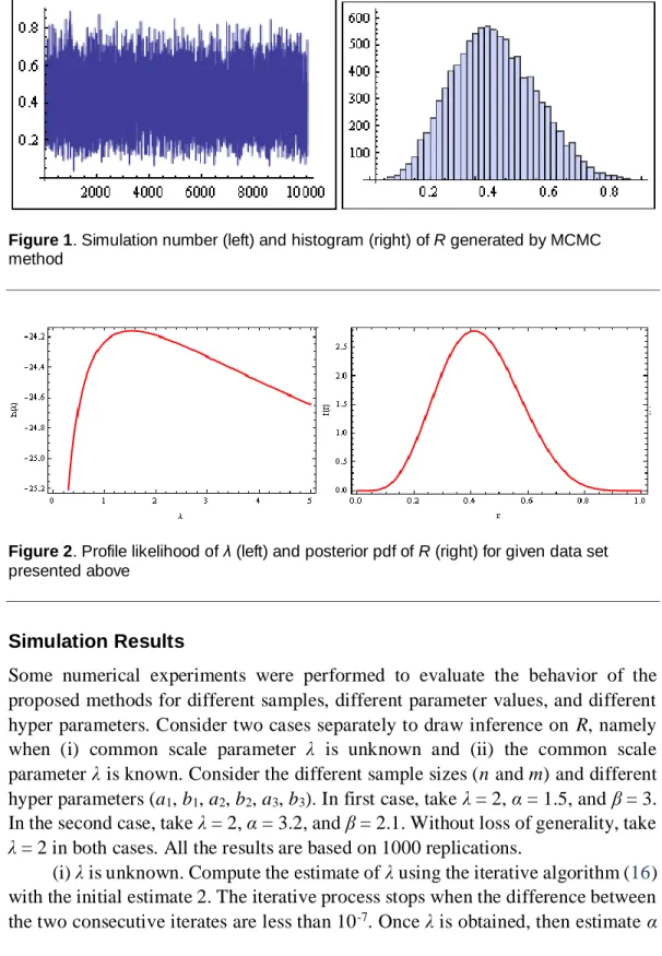
λ is unknown: Based on the above data, plot the profile log-likelihood function of

λ in Figure 2. It is an upside down function and it has a unique maximum. Obtain the MLE of λ using the iterative procedure (16). Using the stopping criterion that the iteration stops whenever two consecutive values are less than 10-6_{, the iteration}

stops after 14 steps and it provides the MLE of



ˆ 1.5232 . Using (13) and (14), obtain the MLEs of



ˆ 1.8958 and ˆ 2.6542, and hence Rˆ 0.4167, from (18). The 95% confidence, credible intervals, and corresponding length are reported in

Table 1 using exact confidence interval, parametric percentile bootstrap methods, and MCMC technique.

Case (2)

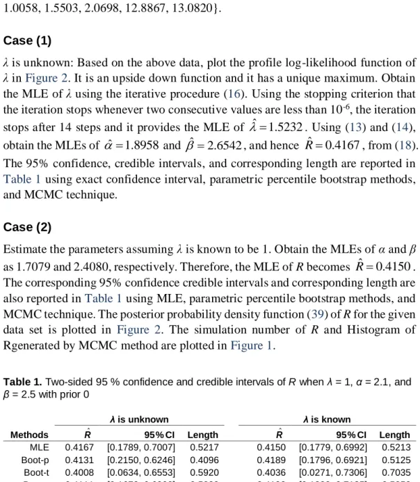
Estimate the parameters assuming λ is known to be 1. Obtain the MLEs of α and β as 1.7079 and 2.4080, respectively. Therefore, the MLE of R becomes Rˆ 0.4150. The corresponding 95% confidence credible intervals and corresponding length are also reported in Table 1 using MLE, parametric percentile bootstrap methods, and MCMC technique. The posterior probability density function (39) of R for the given data set is plotted in Figure 2. The simulation number of R and Histogram of Rgenerated by MCMC method are plotted in Figure 1.

Table 1. Two-sided 95 % confidence and credible intervals of R when λ = 1, α = 2.1, and

β = 2.5 with prior 0

λ is unknown λ is known

Methods R ˆ 95% CI Length R ˆ 95% CI Length

MLE 0.4167 [0.1789, 0.7007] 0.5217 0.4150 [0.1779, 0.6992] 0.5213

Boot-p 0.4131 [0.2150, 0.6246] 0.4096 0.4189 [0.1796, 0.6921] 0.5125

Boot-t 0.4008 [0.0634, 0.6553] 0.5920 0.4036 [0.0271, 0.7306] 0.7035

Figure 1. Simulation number (left) and histogram (right) of R generated by MCMC method

Figure 2. Profile likelihood of λ (left) and posterior pdf of R (right) for given data set

presented above

Simulation Results

Some numerical experiments were performed to evaluate the behavior of the proposed methods for different samples, different parameter values, and different hyper parameters. Consider two cases separately to draw inference on R, namely when (i) common scale parameter λ is unknown and (ii) the common scale parameter λ is known. Consider the different sample sizes (n and m) and different hyper parameters (a1, b1, a2, b2, a3, b3). In first case, take λ = 2, α = 1.5, and β = 3.

In the second case, take λ = 2, α = 3.2, and β = 2.1. Without loss of generality, take

λ = 2 in both cases. All the results are based on 1000 replications.

and β using (13) and (14), respectively. Finally, obtain the MLE of R using (18). To find the Bayes MCMC estimates, use the non-informative gamma priors for the three parameters (we call it prior 0). Non-informative prior (a1 = b1 = a2 = b2 = a3 = b3 = 0) provides prior distributions which are not proper.

Also use informative priors, including prior 1, a1 = 2, b1 = 1, a2 = 3, b2 = 2, a3 = 3,

and b3 = 1, with the values of previous parameters and compute the Bayes estimates

and 95% probability intervals based on 10,000 MCMC samples (discard the first 1,000 values as ‘burn-in’). The average Bayes estimates, means squared errors (MSEs), coverage percentages, and average probability interval lengths based on 1000 replications are reported in Table 2.

(ii) λ is known. Obtain the estimates of R by using the ML method and Lindley's approximation approach. Calculate the exact confidence intervals and HPD interval of R, using the same non-informative prior (prior 0) and an informative prior, including (prior 1) to compute the average estimates of R, MSEs, coverage percentages, and average probability interval lengths based on 1,000 replications. The results are reported in Table 3.

Table 2. Simulation results and estimation of the parameters

MLE Bayes using MCMC

(n, m) RExact Mean MSE Mean MSE Length Coverage

λ = 2, α = 1.5, β = 3 using prior 0 (5, 5) 0.3333 0.3184 0.0205 0.3757 0.0115 0.5311 0.9900 (6, 6) 0.3206 0.0203 0.3742 0.0113 0.4863 0.9810 (7, 6) 0.3227 0.0182 0.3696 0.0111 0.4807 0.9750 (7, 7) 0.3459 0.0169 0.3881 0.0110 0.4617 0.9900 (8, 7) 0.3133 0.0154 0.3735 0.0107 0.4431 0.9850 (8, 8) 0.3286 0.0146 0.3775 0.0106 0.4323 0.9950 (9, 8) 0.3326 0.0141 0.3809 0.0104 0.4211 0.9750 (9, 9) 0.3184 0.0140 0.3624 0.0089 0.4004 0.9550 (10, 9) 0.3172 0.0131 0.3682 0.0087 0.3944 0.9550 (10, 10) 0.3224 0.0126 0.3622 0.0082 0.3819 0.9650 λ = 2, α = 1.5, β = 3 using prior 1 (5, 5) 0.3333 0.3269 0.0202 0.3766 0.0055 0.4399 0.9930 (6, 6) 0.3203 0.0201 0.3698 0.0053 0.4104 0.9950 (7, 6) 0.3246 0.0184 0.3812 0.0052 0.4076 0.9950 (7, 7) 0.3242 0.0151 0.3651 0.0048 0.3895 0.9760 (8, 7) 0.3330 0.0149 0.3780 0.0047 0.3867 0.9950 (8, 8) 0.3378 0.0148 0.3727 0.0045 0.3744 0.9770 (9, 8) 0.3262 0.0146 0.3689 0.0042 0.3653 0.9900 (9, 9) 0.3352 0.0131 0.3663 0.0041 0.3578 0.9660 (10, 9) 0.3335 0.0127 0.3712 0.0039 0.3525 0.9850

Table 3. Simulation results and estimation of the parameters

MLE Bayes using Lindely

(n, m) RExact Mean MSE Length Coverage Mean MSE Length Coverage

λ = 2, α = 3.2, β = 2.1 using prior 0 (5, 5) 0.6038 0.6407 0.0462 0.4535 0.9550 0.6276 0.0393 0.5851 0.9900 (6, 6) 0.6334 0.0373 0.4361 0.9310 0.6298 0.0286 0.5787 0.9950 (7, 6) 0.5954 0.0369 0.4356 0.9450 0.6356 0.0266 0.5308 0.9700 (7, 7) 0.6288 0.0264 0.4259 0.9600 0.6194 0.0224 0.5294 0.9750 (8, 7) 0.6176 0.0235 0.4162 0.9450 0.6211 0.0219 0.5122 0.9650 (8, 8) 0.6129 0.0213 0.4146 0.9280 0.6241 0.0215 0.4941 0.9800 (9, 8) 0.6099 0.1869 0.4100 0.9330 0.6197 0.0162 0.4677 0.9550 (9, 9) 0.6245 0.0176 0.3930 0.9010 0.6407 0.0149 0.4512 0.9390 (10, 9) 0.6021 0.0170 0.3922 0.8990 0.6378 0.0078 0.4189 0.9400 (10, 10) 0.6059 0.0165 0.3820 0.9090 0.6395 0.0052 0.3972 0.9600 λ = 2, α = 3.2, β = 2.1 using prior 0 (5, 5) 0.6038 0.5997 0.0454 0.4732 0.9610 0.6084 0.0251 0.5933 0.9450 (6, 6) 0.5964 0.0397 0.4469 0.9800 0.5832 0.0245 0.5532 0.9230 (7, 6) 0.6156 0.0332 0.4348 0.9120 0.5985 0.0214 0.5159 0.9200 (7, 7) 0.6001 0.0327 0.4221 0.9330 0.5979 0.0207 0.5144 0.9450 (8, 7) 0.6077 0.0260 0.4201 0.9350 0.6193 0.0168 0.5083 0.9450 (8, 8) 0.6065 0.0232 0.4131 0.9050 0.6115 0.0162 0.4899 0.9600 (9, 8) 0.6236 0.0191 0.4022 0.9010 0.6261 0.0136 0.4570 0.9850 (9, 9) 0.6201 0.0157 0.3986 0.9200 0.6283 0.0130 0.4047 0.9640 (10, 9) 0.6029 0.0111 0.3930 0.9050 0.6296 0.0089 0.3995 0.9540 (10, 10) 0.6016 0.0093 0.3822 0.9150 0.6194 0.0051 0.3755 0.9600

Conclusion

The problem of estimating R = P[Y < X] for the Lomax distributions was addressed, and classical and MCMC Bayesian analysis for R were developed when both samples on X and Y are in the form of upper record values, observed from the Lomax distribution with different one shape parameter. The general case when all the parameters are unknown was considered, and when the common scale parameter was known. In the first case, the MCMC method provided an alternative method for parameters estimation of the Lomax distribution and, also, for obtaining both point and interval estimators of the stress-strength reliability model R. It is more flexible when compared with the traditional methods, such as MLE, based on the set of upper record values. It is hoped this investigation will be useful for researchers dealing with the kind of data considered.

 When the common scale parameter λ is unknown, it is observed that the Bayes estimator using MCMC technique works quite well. The MCMC sample were used to construct confidence intervals and that also works quite well. When the common scale parameter λ is known, the maximum likelihood estimator and Bayes estimators were proposed based on the approximate method of Lindley. The confidence interval based on the exact distribution of the MLE works quite very well. Also, a HPD interval was recommended

 Tables 2 and 3 show that, when m = n and m, n increase, then MSEs and average confidence interval lengths, credible interval lengths of the MLEs, and Bayes estimators decrease, and that the coverage percentages are reached to the nominal level in most cases

 From Tables 2 and 3, it is clear that the Bayes estimators based on informative priors (prior 1) perform much better than the Bayes estimators based on non-informative priors (prior 0) or MLEs in terms of biases, MSEs, and lengths of credible intervals.

References

Abd Ellah, A. H. (2003). Bayesian one sample prediction bounds for the Lomax distribution. Indian Journal Pure and Applied Mathematics, 34(1), 101-109.

Abd Ellah, A. H. (2006). Comparison of estimates using record statistics from Lomax model: Bayesian and non Bayesian approaches. Journal of Statistical Research of Iran, 3(2), 139-158. Retrieved from

http://en.journals.sid.ir/ViewPaper.aspx?ID=134210

Arnold, B. C., Balakrishnan, N., & Nagaraja, H. N. (1998). Records. New York, NY: Wiley.

Baklizi, A., & El-Masri A. Q. (2004). Shrinkage estimation of P(X<Y) in the exponential case with common location parameter. Metrika, 59(2), 163-171. doi:

10.1007/s001840300277

Baklizi, A. (2008a). Estimation of Pr(X < Y) using record values in the one and two parameter exponential distributions. Communications in Statistics – Theory and Methods, 37(5), 692-698. doi: 10.1080/03610920701501921

Baklizi, A. (2008b). Likelihood and Bayesian estimation of Pr(X < Y) using lower record values from the generalized exponential distribution. Computational

Chen, M. H., Shao, Q. M., & Ibrahim, J. G. (2000). Monte Carlo methods in Bayesian computation. New York, NY: Springer-Verlag.

Efron, B. (1982). The jackknife, the bootstrap and other resampling plans.

CBMS-NSF Regional Conference Series in Applied Mathematics, CB38. doi:

10.1137/1.9781611970319.fm

Gentle, J. E. (1998). Random number generation and Monte Carlo methods. New York, NY: Springer.

Gupta, R. C., & Peng, C. (2009). Estimating reliability in proportional odds ratio models. Computational Statistics & Data Analysis, 53(4), 1495-1510. doi:

10.1016/j.csda.2008.10.014

Habibullah, M., & Ahsanullah, M. (2000). Estimation of parameters of a Pareto distribution by generalized order statistics. Communication in Statistics – Theory and Methods, 29(7), 1597-1609. doi: 10.1080/03610920008832567

Hall, P. (1988). Theoretical comparison of bootstrap confidence intervals.

TheAnnals of Statistics, 16(3), 927-953. Available from

http://www.jstor.org/stable/2241604

Hastings, W. K. (1970). Monte Carlo sampling methods using Markov chains and their applications. Biometrika, 57(1), 97-109. doi:

10.1093/biomet/57.1.97

Kakade, C. S., Shirke, D. T., & Kundu, D. (2008). Inference for P(Y<X)in exponentiated Gumbel distribution, Journal of Statistics and Applications, 3(1-2): 121-133.

Kotz, S., Lumelskii, Y., & Pensky, M. (2003). The stress-strength model and its generalizations: Theory and applications: P(X<Y). Singapore: World Scientific.

Krishnamoorthy, K., Mukherjee, S., & Guo, H. (2007). Inference on reliability in two-parameter exponential stress-strength model. Metrika, 65(3), 261-273. doi: 10.1007/s00184-006-0074-7

Kundu, D., & Gupta, R. D. (2005). Estimation of P[Y < X] for generalized exponential distribution. Metrika, 61(3), 291-308. doi: 10.1007/s001840400345

Kundu, D., & Gupta, R. D. (2006). Estimation of P[Y < X] for Weibull distributions. IEEE Transactions on Reliability, 55(2), 270-280. doi:

10.1109/TR.2006.874918

three-Lindley, D. V. (1980). Approximate Bayesian methods. Trabajos de Estadistica Y de Investigacion Operativa, 31(1), 223-237. doi:

10.1007/BF02888353

Lomax, K. S. (1954) Business failure: Another example of the analysis of the failure data. Journal of the American Statistical Association, 49(268), 847-852. doi: 10.1080/01621459.1954.10501239

Metropolis, N., Rosenbluth, A. W., Rosenbluth, M. N., Teller, A. H., & Teller, E. (1953). Equations of state calculations by fast computing machines. The Journal of Chemical Physics, 21(6), 1087-1091. doi: 10.1063/1.1699114

Mokhlis, N. A. (2005). Reliability of a stress-strength model with Burr type III distributions. Communications in Statistics – Theory and Methods, 34(7), 1643-1657. doi: 10.1081/STA-200063183

Nadarajah, S. (2003). Reliability for lifetime distributions. Mathematical and Computer Modelling, 37(7-8), 683-688. doi: 10.1016/S0895-7177(03)00074-8

Nadarajah, S. (2004a). Reliability for logistic distributions. Elektronnoe Modelirovanie, 26(3), 65-82.

Nadarajah, S. (2004b). Reliability for Laplace distributions. Mathematical Problems in Engineering, 2004(2), 169-183. doi: 10.1155/S1024123X0431104X

Nadarajah, S. (2005a). Reliability for some bivariate beta distributions.

Mathematical Problems in Engineering, 2005(1), 101-111. doi:

10.1155/MPE.2005.101

Nadarajah, S. (2005b). Reliability for some bivariate gamma distributions.

Mathematical Problems in Engineering, 2005(2), 151-163. doi:

10.1155/MPE.2005.151

Nadarajah, S., & Kotz, S. (2006). Reliability for some bivariate exponential distributions. Mathematical Problems in Engineering, 2006. doi:

10.1155/MPE/2006/41652

Rezaeia, S., Tahmasbib, R., & Mahmoodi, M. (2010). Estimation of P[Y<X] for generalized Pareto distribution. Journal of Statistical Planning and Inference, 140(2), 480-494. doi: 10.1016/j.jspi.2009.07.024

Robert, C. P., & Casella, G. (2004). Monte Carlo statistical methods (2nd ed.). New York, NY: Springer.

Saraçoglu, B., & Kaya, M. F. (2007). Maximum likelihood estimation and confidence intervals of system reliability for Gompertz distribution in

stress-strength models. Selçuk Journal of Applied Mathematics, 8(2), 25-36. Retrieved from http://sjam.selcuk.edu.tr/sjam/article/view/188

Shoukri, M. M., Chaudhary, M. A., & Al-Halees, A. (2005). Estimating

P(Y < X) when X and Y are paired exponential variables. Journal of Statistical Computation and Simulation, 75(1), 25-38. doi: 10.1080/00949650410001653142

Soliman, A. A., & Al-Aboud, F. M. (2008). Bayesian inference using record values from Rayleigh model with application. European Journal of Operational Research, 185(2), 659-672. doi: 10.1016/j.ejor.2007.01.023

Surles, J. G., & Padgett, W. J. (2001). Inference for reliability and stress-strength for a scaled Burr-type X distribution. Lifetime Data Analysis, 7(2), 187-200. doi: 10.1023/A:1011352923990

Upadhyay, S. K., & Peshwani, M. (2003). Choice between Weibull and lognormal models: A simulation based Bayesian study. Communication in Statistics – Theory and Methods, 32(2), 381-405. doi: 10.1081/STA-120018191

Wang, L., & Shi, Y. (2010). Empirical Bayes inference for the Burr model based on records. Applied Mathematical Sciences, 4(34), 1663-1670. Retrieved from