Sparse and low rank signal recovery with partial knowledge

(1)

Dissertations

2015

Sparse and low rank signal recovery with partial

knowledge

Jinchun Zhan

Iowa State University

Follow this and additional works at:https://lib.dr.iastate.edu/etd Part of theElectrical and Electronics Commons

This Dissertation is brought to you for free and open access by the Iowa State University Capstones, Theses and Dissertations at Iowa State University Digital Repository. It has been accepted for inclusion in Graduate Theses and Dissertations by an authorized administrator of Iowa State University Digital Repository. For more information, please contactdigirep@iastate.edu.

Recommended Citation

Zhan, Jinchun, "Sparse and low rank signal recovery with partial knowledge" (2015).Graduate Theses and Dissertations. 14869.

(2)

by Jinchun Zhan

A dissertation submitted to the graduate faculty in partial fulfillment of the requirements for the degree of

DOCTOR OF PHILOSOPHY

Major: Electrical Engineering

Program of Study Committee: Namrata Vaswani, Major Professor

Aditya Ramamoorthy Nicola Elia Leslie Hogben Kris De Brabanter

Iowa State University Ames, Iowa

2015

(3)

DEDICATION

I would like to dedicate this dissertation to my family without whose support I would not have been able to complete this work.

(4)

LIST OF TABLES

Table 3.1 Speed comparison of different algorithms. Sequence length refers to

(10)

LIST OF FIGURES

Figure 1.1 Slow support change in medical image sequences. We used the two-level Daubechies-4 2D discrete wavelet transform (DWT) as the spar-sity basis. Since real image sequences are only approximately sparse,

we use Nt to denote the 99%-energy support of the DWT of these

sequences. The support size,|Nt|, was 6-7% of the image size for both sequences. We plot the number of additions (left) and the number of removals (right) as a fraction of_|N_t|. Notice that all changes are less than 2% of the support size. . . 5

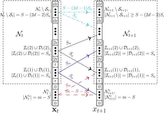
Figure 2.1 Signal Change Assumptions 1 (Values inside rectangular denote magnitudes.) . . . 25

Figure 2.2 Signal Change Assumptions 2 (Values inside rectangular denote magnitudes.) . . . 34

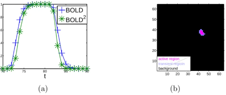
Figure 2.3 (a): plot of the BOLD signal and of its square. (b): active, transient and inactive brain regions. . . 46

Figure 2.4 Error Comparison with Fixed Measurement Matrix. “CS” in the figures refers to noisy `1, i.e. the solution of (2.1) at each time. . 50

Figure 2.5 Error Comparison with Time Varying Measurement Matrices. “CS” in the figures refers to noisy `1, i.e. the solution of (2.1)

at each time. . . 50

(11)

Figure 3.1 Comparison with increasing rextra (n1 = 200, d = 200, n2 = 120,

m = 0.075n1n2, r = 20, r0 = 18, rnew = 2). In (b), we plot the

value ofρr needed to satisfy (3.1), (3.2), (3.3) and (3.5), (3.6), (3.7).

We denote the respective values of ρr by ρr([G Unew]), ρr(Vnew),

ρr(UnewVnew), ρr(U), ρr(V) and ρr(UV). Notice that ρr(UV) is

the largest, i.e. (3.7) is the hardest to satisfy. Notice also that

ρr(mod-PCP) = max{ρr([G Unew]), ρr(Vnew), ρr(UnewVnew)} is sig-nificantly smaller thanρr(PCP) = max{ρr(U), ρr(V), ρr(UV)}. . . 72 Figure 3.2 Comparison with increasing rnew (n1 = 200, d = 200, n2 = 120,

m= 0.075n1n2,r= 30, rextra= 5). . . 72

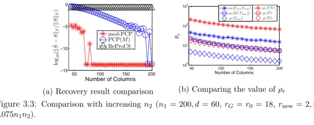
Figure 3.3 Comparison with increasing n2 (n1 = 200, d = 60, rG = r0 = 18,

rnew= 2, m= 0.075n1n2). . . 73

Figure 3.4 Phase transition plots with rnew=b0.15rc, rextra=b0.15rc, n1 =

400 . . . 74

Figure 3.5 Yale Face Image result comparison . . . 75

Figure 3.6 NRMSE of sparse part comparison with online model (n= 256,J = 3,

r0 = 40,t0 = 200, cj,new = 4,cj,old= 4,j = 1,2,3) . . . 75

Figure 3.7 Lake sequence NMSE comparison. (a) shows comparisons for one slow-moving foreground object; (b) shows comparisons for a large number of small-sized fast-moving foreground objects (total foreground

(12)

Figure 4.1 The first column shows the video of a moving rectangular object a-gainst moving lake waters’ background. The object and its motion are simulated while the background is real. In the next two columns,

we show the recovered background (ˆ`t) and the recovered foreground

support ( ˆTt) using Automatic ReProCS-cPCA (labeled ReProCS in

the figure). The algorithm parameters are set differently for the

ex-periments (see Sec. 4.8) than in our theoretical result. Notice that

the foreground support is recovered mostly correctly with only a few extra pixels and the background appears correct too (does not contain the moving block). The quantitative comparison is shown later in Fig.

4.4. The next few columns show background and foreground-support

recovery using some of the existing methods discussed in Sec. 4.1.1. . 82

Figure 4.2 Examples of Model 4. (a) shows a 1D object of length s that moves

by at least s/3 pixels at least once every 5 frames (i.e., ρ = 3 and

β = 5). (b) shows the object moving bys pixels at every frame (i.e.,

ρ= 1 and β = 1). (b) is an example of the best case for our result

-the case with -the smallestρ, β (_Tt’s mutually disjoint) . . . 87

Figure 4.3 A diagram of Model 5 . . . 90

Figure 4.4 Average error comparisons for fully simulated data and for the

(13)

ACKNOWLEDGEMENTS

Firstly, I would like to thank Dr. Namrata Vaswani for her patience, guidance and support throughout my research and preparation for this dissertation. With her help, I can complete and enjoy my research.

And I would like to thank Dr. Aditya Ramamoorthy, Dr. Nicola Elia, Dr. Leslie Hogben, and Dr Kris De Brabanter for their support and comments to perfect my research and this dissertation.

Also I would like to thank all my friends who make my life in Iowa State University more enjoyable.

Finally I would like to thank my family, especially Yu Jie, without whose support, I cannot complete my research.

(14)

ABSTRACT

In the first part of this work, we study sparse recovery problem in the presence of bounded noise. We obtain performance guarantees for modified-CS and for its improved version, modified-CS-Add-LS-Del, for recursive reconstruction of a time sequence of s-parse signals from a reduced set of noisy measurements available at each time. Under mild assumptions, we show that the support recovery error and reconstruction error of both algorithms are bounded by a time-invariant and small value at all times.

In the second part of this work, we study batch sparse recovery problem in the presence of large and low rank noise, which is also known as the problem of Robust Principal Components Analysis (RPCA). In recent work, RPCA has been posed as a problem of recovering a low-rank matrix Land a sparse matrix S from their sum,M:=

L+S and a provably exact convex optimization solution called PCP has been proposed. We study the following problem. Assume that we have a partial estimate of the column space of the low rank matrix L, we propose here a simple but useful modification of the PCP idea, called modified-PCP, that allows us to use this knowledge. We derive its correctness result which shows that modified-PCP indeed requires significantly weaker incoherence assumptions than PCP, when the available subspace knowledge is accurate. In the third part of this work, we study the “online” sparse recovery problem in the presence of low rank noise and bounded noise, which is also known as the “online” RPCA problem. Here we study a more general version of this problem, where the goal is to recover low rank matrix L and sparse matrix S from M:= L+S+W and W is the matrix of unstructured small noise. We develop and study a novel “online” RPCA algorithm based on the recently introduced Recursive Projected Compressive Sensing

(15)

(ReProCS) framework. The key contribution is a correctness result for this algorithm under relatively mild assumptions.

(16)

CHAPTER 1. INTRODUCTION

The static sparse reconstruction problem has been studied for a while [2, 3, 4, 5, 6]. The papers on compressive sensing (CS) from 2005 [7,8, 9, 10,11,12] (and many other more recent works) provide the missing theoretical guarantees – conditions for exact recovery and error bounds when exact recovery is not possible. In more recent works, the problem of recursively recovering a time sequence of sparse signals, with slowly changing sparsity patterns has also been studied [13, 1, 14, 15, 16, 17, 18, 19]. By “recursive” reconstruction, we mean that we want to use only the current measurements’ vector and the previous reconstructed signal to recover the current signal. This problem occurs in many applications such as real-time dynamic magnetic resonance imaging (MRI); single-pixel camera based real-time video imaging; recursively separating the region of the brain that is activated in response to a stimulus from brain functional MRI (fMRI) sequences [20] and recursively extracting sparse foregrounds (e.g. moving objects) from slow-changing (low-dimensional) backgrounds in video sequences [21]. For other potential applications, see [22, 23].

An important assumption introduced and empirically verified in [13, 1] is that for many natural signal/image sequences, the sparsity pattern (support set of its projection into the sparsity basis) changes slowly over time. In [14], the authors exploited this fact to reformulate the above problem as one of sparse recovery with partially known support and introduced a solution approach called modified-CS. Given the partial support knowledge

T, modified-CS tries to find a signal that is sparsest outside of _T among all signals that satisfy the data constraint. Exact recovery conditions were obtained for modified-CS

(17)

and it was argued that these are weaker than those for simple `1 minimization (basis

pursuit) under the slow support change assumption. Related ideas for support recovery with prior knowledge about the support entries, that appeared in parallel, include [24], [25]. All of [14], [24] and [25] studied the noise-free measurements’ case. Later work includes [26, 27].

Error bounds for modified-CS for noisy measurements were obtained in [28], [29], [30]. When modified-CS is used for recursive reconstruction, these bounds tell us that the reconstruction error bound at the current time is proportional to the support recovery error (misses and extras in the support estimate) from the previous time. Unless we impose extra conditions, this support error can keep increasing over time, in which case the bound is not useful. Thus, for recursive reconstruction, the important question is, under what conditions can we obtain time-invariant bounds on the support error (which will, in turn, imply time-invariant bounds on the reconstruction error)? In other words, when can we ensure “stability” over time? Notice that, even if we did nothing, i.e. we set ˆxt = 0, the support error will be bounded by the support size. If the support size is bounded, then this is a naive stability result too, but is not useful. Here, we look for results in which the support error bound is small compared to the support size.

Stability over time has not been studied much for recursive recovery of sparse signal sequences. To the best of our knowledge, it has only been addressed in [1], and in very recent work [19]. The result of [19] is for exact dynamic support recovery in the noise-free case and it studies a different problem: the MMV version of the recursive recovery problem. The result from [1] for Least Squares CS-residual (LS-CS) stability) holds under mostly mild assumptions; its one limitation is that it assumes that support changes occur every pframes. But from testing the slow support change assumption for real data (medical image sequences), it has been observed that support changes usually occur at every time, e.g. Fig. 1.1. This important case is the focus of current work. We explain the differences of our results w.r.t. the LS-CS result in detail later in Sec2.5.5.

(18)

Principal Components Analysis (PCA) is a widely used dimension reduction tech-nique that finds a small number of orthogonal basis vectors, called principal components (PCs), along which most of the variability of the dataset lies. Accurately computing the PCs in the presence of outliers is called robust PCA. Outlier is a loosely defined term that refers to any corruption that is not small compared to the true data vector and that occurs occasionally. As suggested in [31], an outlier can be nicely modeled as a sparse vector. The robust PCA problem occurs in various applications ranging from video analysis to recommender system design in the presence of outliers, e.g. for Netflix movies, to anomaly detection in dynamic networks [32]. In video analysis, background image sequences are well modeled as forming a low-rank but dense matrix because they change slowly over time and the changes are typically global. Foreground is a sparse image consisting of one or more moving objects. In recent work, Candes et al and Chan-drasekharan et al [32,33] posed the robust PCA problem as one of separating a low-rank matrix L (true data matrix) and a sparse matrix S (outliers’ matrix) from their sum,

M := L+S. They showed that by solving the following convex optimization called principal components’ pursuit (PCP)

minimize_L˜_,_S˜ kL˜k∗+λkS˜k1

subject to L˜+ ˜S=M

(1.1)

it is possible to recover L and S exactly with high probability under mild assumptions. This was among the first recovery guarantees for a practical (polynomial complexity) robust PCA algorithm. Since then, the batch robust PCA problem, or what is now also often called the sparse+low-rank recovery problem, has been studied extensively, e.g. see [34, 35,36, 37, 38,39, 40, 41, 42,43].

In this work, we introduce modified-CS-add-LS-del which is a modified-CS based algorithm for recursive recovery with an improved support estimation step and we explain how to set its parameters in practice. The main contribution of this work is to obtain conditions for stability of modified-CS and modified-CS-add-LS-del for recursive recovery

(19)

of a time sequence of sparse signals. Under mild assumptions, we show that the support recovery error and the reconstruction error of both algorithms is bounded by a time-invariant value at all times. The support error bound is proportional to the maximum allowed support change size. Under slow support change, this bound is small compared to the support size, making our result meaningful. Similar arguments can be made for the reconstruction error also. The assumptions we need are: weaker restricted isometry property (RIP) conditions [10] on the measurement matrix than what`1minimization for

noisy data (henceforth referred to asnoisy `1) needs; bounded cardinality of the support

and support change; all but a small number of existing nonzero entries are above a threshold in magnitude; appropriately set support estimation thresholds; and a special start condition. Here and elsewhere in the paper noisy `1 (or simple CS) refers to the

solution of (2.1).

A second main contribution of this work is to show two examples of signal change assumptions under which the required conditions hold and prove stability results for these. The first case is a simple signal change model that helps to illustrate the key ideas and allows for easy comparison of the results. The second set of assumptions is realistic, but more complicated to state. We use MRI image sequences to demonstrate that these assumptions are indeed valid for real data. The essential requirement in both cases is that, for any new element that is added to the support, either its initial magnitude is large enough, or for the first few time instants, its magnitude increases at a large enough rate; and a similar assumption for magnitude decrease and removal from the support.

LetSbe the bound on the maximum support size andSa the bound on the maximum number of support additions or removals. All our results require s-RIP to hold with

s=S+kSa where k is a constant. On the other hand, noisy `1 needss-RIP fors = 2S

[12] which is a stronger requirement when Sa S (slow support change).

In the second part we study the following problem. Suppose that we have a partial estimate of the column space of the low rank matrix L. How can we use this information

(20)

Figure 1.1: Slow support change in medical image sequences. We used the two-level Daubechies-4 2D discrete wavelet transform (DWT) as the sparsity basis. Since real image

sequences are only approximately sparse, we use Nt to denote the 99%-energy support of the

DWT of these sequences. The support size,_|N_t|, was 6-7% of the image size for both sequences.

We plot the number of additions (left) and the number of removals (right) as a fraction of|Nt|.

Notice that all changes are less than 2% of the support size.

to improve the PCP solution, i.e. allow recovery under weaker assumptions? We propose here a simple but useful modification of the PCP idea, called modified-PCP, that allows us to use this knowledge. We derive its correctness result (Theorem3.1.1) that provides explicit bounds on the various constants and on the matrix size that are needed to ensure exact recovery with high probability. Our result is used to argue that modified-PCP indeed requires significantly weaker incoherence assumptions than modified-PCP, as long as the available subspace knowledge is accurate. To prove the result, we use the overall proof approach of [32] with some changes (see Sec 3.3).

An important problem where partial subspace knowledge is available is in online or recursive robust PCA for sequentially arriving time series data, e.g. for video based foreground and background separation. In this case, as explained in [44], the subspace spanned by a set of consecutive columns ofLdoes not remain fixed, but instead changes over time and the changes are gradual. Also, often an initial short sequence of low-rank only data (without outliers) is available, e.g. in video analysis, it is easy to get an initial background-only sequence. For this application, modified-PCP can be used to design a piecewise batch solution that will be faster and will require weaker assumptions for exact recovery than PCP. This is made precise in Corollary 3.2.1 and the discussion below it. We show extensive simulation comparisons and some real data comparisons of modified-PCP with modified-PCP and with other existing robust PCA solutions from literature. The

(21)

im-plementation requires a fast algorithm for solving the modified-PCP program. This is developed by modifying the Inexact Augmented Lagrange Multiplier Method [45] and using the idea of [46, 47] for the sparse recovery step. The real data comparisons are for a face reconstruction / recognition application in the presence of outliers, e.g. eye-glasses or occlusions, that is also discussed in [32].

When RPCA needs to be solved in a recursive fashion for sequentially arriving data vectors it is referred to as online RPCA. Our “online” RPCA formulation assumes that (i) a short sequence of outlier-free (sparse component free) data vectors is available or that there is another way to get an estimate of the initial subspace of the true data (without outliers); and that (ii) the subspace from which `t is generated is fixed or changes slowly over time. We put “online” in quotes here to stress that our problem formulation uses extra assumptions beyond what are used by RPCA (or batch RPCA). A key application of RPCA is the problem of separating a video sequence into foreground and background layers [32]. Video layering is a key first step to simplifying many video analytics and computer vision tasks, e.g., video surveillance (to track moving foreground objects), background video recovery and subspace tracking in the presence of frequent foreground occlusions or low-bandwidth mobile video chats or video conferencing (can transmit only the foreground layer). In videos, the foreground typically consists of one or more moving persons or objects and hence is a sparse image. The background images (in a static camera video) usually change only gradually over time, e.g., moving lake waters or moving trees in a forest, and the changes are global [32]. Hence they are well modeled as being dense and lying in a low-dimensional subspace that is fixed or slowly changing. Other applications where RPCA occurs include recommendation system design, survey data analysis, anomaly detection in dynamic social (or computer) networks [32] and dynamic magnetic resonance imaging (MRI) based region-of-interest tracking [48].

(22)

1.1 Notation and Problem Definition

1.1.1 Notation

We use bold lowercase for vectors, bold uppercase for matrices, calligraphic uppercase for sets or corresponding linear space.

We let [1, m] := [1,2, . . . m]. We let _∅denote an empty set. We use _Tc _{to denote the} complement of a setT w.r.t. [1, m], i.e. Tc_:=_{_i_∈_[1_{, m}_{] :}_{i /}_{∈ T }}_{. We use}_{|T |}_{to denote} the cardinality of T. The set operations ∪, ∩, \ have their usual meanings (recall that

A \ B :=A ∩ Bc_{). If two sets}_B_,_C _{are disjoint, we just write}_{D ∪ B \ C} _{instead of writing} (_{D ∪ B})_{\ C}.

For a vector, x, and a set, _T, x_T denotes the _{|T |} length sub-vector containing the elements of x corresponding to the indices in the set _T. _kx_kk denotes the `k norm of a vector x. If just _kx_k is used, it refers to _kx_k2. Similarly, for a matrix M, kMkk denotes its induced k-norm, while just kM_k refers to kM_k2. M0 denotes the transpose

of M and M† denotes the Moore-Penrose pseudo-inverse of M (when M is full column rank, M† := (M0M)−1_M0_{). Also,} _M

T denotes the sub-matrix obtained by extracting the columns of M corresponding to indices in_T.

We refer to the left (right) hand side of an equation or inequality as LHS (RHS). For a matrix X, we denote by X∗ the transpose of X; denote by_kX_k_∞ the `_∞ norm of X reshaped as a long vector, i.e., maxi,j_|Xij|; denote by kXk the operator norm or 2-norm; denote bykX_kF the Frobenius norm; denote by kXk∗ the nuclear norm; denote bykX_k1 the `1 norm of X reshaped as a long vector.

Let PI denote the identity operator, i.e., PI(Y) = Y for any matrix Y. Let kPAk denote the operator norm of operator _P_A, i.e., _k_P_A_k= sup_{k_X_k_F₌₁_}_k_P_AX_k_F; let _hX,Y_i

denote the Euclidean inner product between two matrices, i.e., trace(X∗Y); let sgn(X) denote the entrywise sign of X. We let _PΘ denote the orthogonal projection onto linear

(23)

0_}. We also use Ω to denote the subspace spanned by all matrices supported on Ω. By Ω _∼ Ber(ρ) we mean that any matrix index (i, j) has probability ρ of being in the support independent of all others.

Given two matrices B and B2, [B B2] constructs a new matrix by concatenating

matrices B and B2 in the horizontal direction. Let Brem be a matrix containing some

columns ofB. ThenB_\B_rem is the matrix B with columns in B_rem removed.

We say that U is a basis matrix if U∗U= Iwhere Iis the identity matrix. We use

ei to refer to the ith column I.

We use the interval notation [a, b] to mean all of the integers betweena and b, inclu-sive, and similarly for [a, b) etc. For a set T, |T | denotes its cardinality and ¯T denotes its complement set. We use ∅ to denote the empty set. For a vector x, x_T is a smaller vector containing the entries of x indexed by T. Define I_T to be an n× |T | matrix of those columns of the identity matrix indexed by T. For a matrix A, define A_T :=AI_T. We use 0 _{to denote transpose. The} _l

p-norm of a vector and the induced lp-norm of a matrix are denoted by _{k · k}p. We refer to a matrix with orthonormal columns as a basis

matrix. Thus, for a basis matrix P, P0P=I. For matrices P, Q where the columns of

Q are a subset of the columns of P, P_\Q refers to the matrix of columns inP and not in Q. For a matrix H,HEVD= UΛU0 denotes its reduced eigenvalue decomposition. For a matrixA, the restricted isometry constant (RIC) δs(A) is the smallest real numberδs such that

(1₋δs)kxk22 ≤ kAxk22 ≤(1 +δs)kxk22

for alls-sparse vectorsx[12]. A vectorxiss-sparse if it hassor fewer non-zero entries. For Hermitian matrices A and B, the notation A B means that B₋A is positive semi-definite. For basis matrices ˆP and P, dif( ˆP,P) := k(I₋PˆPˆ0)P_k2 quantifies error

(24)

1.1.2 Problem definition

The first type of problems that we study here are as following. We assume the following observation model:

yt =Atxt+wt, kwtk ≤ (1.2) where xt is an m length sparse vector with support set Nt, i.e. Nt:={i: (xt)i 6= 0};At is a nt×m measurement matrix; yt is the nt length observation vector at time t (with

nt < m); andwt is the observation noise. For t >0, we fix nt =n.

Our goal is to recursively estimate xt using y1, . . .yt. By recursively, we mean, use

only y_t and the estimate from t₋1, ˆx_t₋₁, to compute the estimate att.

Remark 1.1.1 (Why bounded noise). All results for bounding `1 minimization error

in noise, and hence all results for bounding modified-CS error in noise, either assume a deterministic noise bound and then bound _kˆx₋x_k, e.g., [12], [49], [28, 50], [51]; or

assume unbounded, e.g. Gaussian, noise and then bound_kxˆ₋x_kwith “large” probability,

e.g. [52], [53, Sec IV], [1, Section III-A], [51]. The latter approach is not useful for

recovering a time sequence of sparse signals because the error bound will hold for all

times 0≤t <∞ with probability zero.

One way to get a meaningful error stability result with unbounded, e.g. Gaussian noise, is to compute or bound the expected value of the error at each time, i.e. compute

E[(ˆxt−xt)(ˆxt−xt)0]or bound some norm of it. This is possible to do, for example, for a

Kalman filter applied to a linear system model with additive Gaussian noise; and hence in that case, one can assume Gaussian noise and still get a time-invariant bound on the

expected value of the error under mild assumptions. However, for `1 minimization based

methods, such as modified-CS, there is no easy way to compute or bound the expected value of the error. Moreover, even if one could do this for a given time, it would not tell us anything about the support recovery error (for the given noise sequence realization) and hence would not be useful for analyzing modified-CS.

(25)

As a sidenote, we should point out that, in most applications, the noise is typically bounded (because of finite sensing power available). One often chooses to model the noise as Gaussian because it simplifies performance analysis.

The second type of problems that we study here are as following. We are given a data matrix M_∈_Rn1×n2 _{that satisfies}

M=L+S (1.3)

where S is a sparse matrix with support set Ω and L is a low rank matrix with rank r

and with reduced singular value decomposition (SVD)

L=UΣV∗ (1.4)

We assume that we are given an n1 ×rG basis matrix G so that (I −GG∗)L has rank

smaller than r. The goal is to recover L and S from M usingG.

We explain the above a little more. With G as above, Ucan be rewritten as

U= [(GR_\Uextra)

| {z }

U0

Unew], (1.5)

whereUnew∈Rn1×rnew and U∗newG= 0; Ris a rotation matrix andUextracontains rextra

columns of GR. Let r0 be the number of columns in U0. Then, clearly,r0 =rG−rextra

and r =r0+rnew.

We use Vnew to denote the right singular vectors of the reduced SVD of Lnew :=

(I₋GG∗)L=UnewU∗newL. In other words,

Lnew := (I−GG∗)L SVD

= UnewΣnewV∗new (1.6)

From the above model, it is clear that

(26)

forX =L∗G. We propose to recoverLandSusingGby solving the followingModified PCP (mod-PCP) program

minimize_L˜_new_,_S˜_,_X˜ kL˜newk∗+λkS˜k1

subject to L˜_new+GX˜∗+ ˜S=M

(1.8)

Denote a solution to the above by ˆLnew,Sˆ,Xˆ. Then, L is recovered as ˆL = ˆLnew +

GXˆ∗. Modified-PCP is inspired by an approach for sparse recovery using partial support knowledge called modified-CS [54].

The third type of problems that we study here are as following. At timet we observe a data vector m_t_{∈ R}n that satisfies

mt =`t+xt+wt, for t=ttrain+ 1, ttrain+ 2, . . . , tmax. (1.9)

For t = 1,2, . . . , ttrain, xt = 0, i.e., mt = `t +wt. Here `t is a vector that lies in a low-dimensional subspace that is fixed or slowly changing in such a way that the matrix

Lt:= [`1,`2, . . . ,`t] is a low-rank matrix for all but very small values of t; xt is a sparse (outlier) vector; and wt is small modeling error or noise. We use Tt to denote the support set ofx_t and we useP_t to denote a basis matrix for the subspace from which `t is generated. For t > ttrain, the goal of online RPCA is to recursively estimate `t and its subspace range(Pt), and xt and its support, Tt, as soon as a new data vector mt arrives or within a short delay 1_{. Sometimes, e.g., in video analytics, it is often also desirable}

to get an improved offline estimate of xt and `t when possible. We show that this is an easy by-product of our solution approach.

The initialttrainoutlier-free measurements are used to get an accurate estimate of the

initial subspace via PCA. For video surveillance, this assumption corresponds to having a short initial sequence of background only images, which can often be obtained.

In many applications, it is actually the sparse outlierxtthat is the quantity of interest. The above problem can thus also be interpreted as one of online sparse matrix recovery

1_{By definition, a subspace of dimension} _{r >} _{1 cannot be estimated immediately since it needs at}

(27)

in large but structured noise`tand unstructured small noise wt. The unstructured noise,

wt, often models the modeling error. For example, when some of the corruptions/outliers are small enough to not significantly increase the subspace recovery error, these can be included intowtrather thanxt. Another example is when the`t’s form an approximately low-rank matrix.

1.2 Dissertation Organization

The dissertation is organized as follows. Recursive sparse recovery in bounded noise and corresponding results are introduced in Chapter 2. Batch sparse recovery in large and structured noise and corresponding results are discussed in Chapter 3. Recursive (online) sparse recovery in large and structured noise and bounded noise and correspond results are demonstrated in Chapter 4. Finally, conclusions are summarized in Chapter

(28)

CHAPTER 2. RECURSIVE SPARSE RECOVERY IN

BOUNDED NOISE

2.1 Related Work And Organization

“Recursive sparse reconstruction” also sometimes refers to homotopy methods, e.g. [55], whose goal is to use the past reconstructions and homotopy to speed up the current optimization, but not to achieve accurate recovery from fewer measurements than what noisy`1 needs. The goals in the above works are quite different from ours.

Iterative support estimation approaches (using the recovered support from the first iteration for a second weighted `1 step and doing this iteratively) have been studied in

recent work [56,57,58,59]. This is done for iteratively improving the recovery of asingle

signal.

This chapter is organized as follows. The algorithms – CS and modified-CS-add-LS-del – are introduced in Sec 2.2. This section also includes definitions for certain quantities and sets used later in the paper. In Sec 2.3, we provide stability results for modified-CS and modified-CS-add-LS-del that do not assume anything about signal change over time except a bound on the number of small magnitude nonzero coefficients and a bound on maximum number of support additions or removals per unit time. In Sec 2.4, we give a simple set of signal change assumptions and give stability results for both algorithms under these and other simple assumptions. In Sec 2.5, we do the same for a realistic signal change model. The results are discussed in Sec 2.4.4

(29)

Sec 2.5 are indeed valid for medical imaging data. In Sec 4.4, we explain how to set the algorithm parameters automatically for both modified-CS and modified-CS-add-LS-del. In this section, we also give simulation experiments that back up some of our discussions from earlier sections.

2.2 Modified-CS And Modified-CS-add-LS-del For Recursive

Reconstruction

2.2.1 Modified-CS

Modified-CS was first proposed in [14] as a solution to the problem of sparse recon-struction with partial, and possibly erroneous, knowledge of the support. Denote this “known” support by T. Modified-CS tries to find a signal that is sparsest outside of the set _T among all signals satisfying the data constraint. In the noisy case, it solves minβk(β)Tck₁ s.t. ky_t−Aβk ≤ . For recursively reconstructing a time sequence of

sparse signals, we use the support estimate from the previous time, ˆ_Nt−1, as the set T.

The simplest way to estimate the support is by thresholding the output of modified-CS. We summarize the complete algorithm in Algorithm1.

At the initial time, t = 0, we let T be the empty set, ∅, i.e. we solve noisy `1.

Alternatively, as explained in [14], we can use prior knowledge of the initial signal’s support as the set T at t= 0, e.g. for wavelet sparse images with no (or a small) black background, the set of indices of the approximation coefficients can form the set_T. This prior knowledge is usually not as accurate.

We explain how the parameter α can be set in practice in Sec 2.7.1.

2.2.2 Limitation: biased solution

Modified-CS uses single step thresholding for estimating the support ˆ_Nt. The thresh-old, α, needs to be large enough to ensure that all (or most) removed elements are

(30)

Algorithm 1 Modified-CS

Fort _≥0, do

1. Noisy `1. If t= 0, setTt=∅ and compute ˆxt,modcs as the solution of

min

β k(β)k1 s.t.ky0−A0βk ≤ (2.1) 2. Modified-CS. If t >0, set Tt = ˆNt−1 and compute ˆxt,modcs as the solution of

min β k(β)T

c

tk1 s.t. kyt−Atβk ≤ (2.2)

3. Estimate the Support. Compute ˜_Tt as

˜

Tt={i∈[1, m] :|(ˆxt,modcs)i|> α} (2.3) 4. Set ˆNt= ˜Tt. Output ˆxt,modcs. Feedback ˆNt.

correctly deleted and there are no (or very few) false detections. But this means that the new additions to the support set will either have to be added at a large value, or their magnitude will need to increase to a large value quickly enough to ensure correct detection within a small delay. This issue is further exaggerated by the fact that ˆxt,modcs is a biased estimate of xt. Along Tc

t, the values of ˆxt,modcs will be biased toward zero (because we minimize _k(β)_Tc

tk1), while, along Tt, they may be biased away from zero.

This will create the following problem. The set _Tt contains the set ∆e,t which needs to be deleted. Since the estimates along ∆e,t may be biased away from zero, one will need a higher threshold to delete them. But that would make detection more difficult, especially since the estimates along ∆t⊆ Tc

t will be biased towards zero. A similar issue for noisy CS, and a possible solution (Gauss-Dantzig selector), was first discussed in [52].

2.2.3 Modified-CS with Add-LS-Del

The bias issue can be partly addressed by replacing the support estimation step of Modified-CS by a three step Add-LS-Del procedure summarized in Algorithm 2. It

(31)

involves a support addition step (that uses a smaller threshold -αadd), as in (2.4), followed

by LS estimation on the new support estimate, _Tadd,t, as in (2.5), and then a deletion

step that thresholds the LS estimate, as in (2.6). This can be followed by a second LS estimation using the final support estimate, as in (2.7), although this last step is not critical. The addition step threshold, αadd, needs to be just large enough to ensure that

the matrix used for LS estimation,A_T_add_,t is well-conditioned. If αadd is chosen properly

and ifn is large enough, the LS estimate on_Tadd,t will have smaller error and will be less biased than the modified-CS output. As a result, deletion will be more accurate when done using this estimate. This also means that one can use a larger deletion threshold,

αdel, which will ensure quicker deletion of extras.

Related ideas were introduced in our older work [1, 13] for KF-CS and LS-CS, and in [60, 49] for a greedy algorithm for static sparse reconstruction.

We explain how to automatically set the parameters for both modified-CS-add-LS-del and modified-CS in Sec 2.7.1.

2.2.4 Some definitions

Definition 2.2.1. For any matrix,A, the left S-restricted isometry constant (left-RIC)

δS,left(A) and right S-restricted isometry constant (right-RIC) δS,right(A)are the smallest

real numbers satisfying

(1₋δS,left(A))kck2 ≤ kATck2 ≤(1 +δS,right(A))kck2 (2.8)

for all sets _{T ⊂} [1, m] of cardinality _{|T | ≤} S and all real vectors c of length _{|T |}. The

restricted isometry constant (RIC)[10] is the larger of the two, i.e.,

δS = max{δS,left(A), δS,right(A)}.

Definition 2.2.2. The restricted orthogonality constant (ROC) [10], θS1,S2(A), is the

smallest real number satisfying |c10AT1

0_A

(32)

Algorithm 2 Modified-CS-Add-LS-Del

Fort _≥0, do

1. Noisy `1. If t= 0, setTt=∅ and compute ˆxt,modcs as the solution of (2.1).

2. Modified-CS. Ift >0, set _Tt= ˆNt−1 and compute ˆxt,modcs as the solution of (2.2).

3. Additions / LS. Compute _Tadd,t and the LS estimate using it:

ˆ

At={i:|(ˆxt,modcs)i|> αadd}

Tadd,t=Tt∪Aˆt (2.4) (ˆxt,add)Tadd,t=ATadd,t

†_y

t, (ˆxt,add)Tc

add,t = 0 (2.5)

4. Deletions / LS. Compute ˜Tt and LS estimate using it:

ˆ

Rt={i∈ Tadd,t :|(ˆxt,add)i| ≤αdel}

˜

Tt=Tadd,t\Rˆt (2.6) (ˆx_t)_T˜_t=A_T˜_t†yt, (ˆxt)_T˜c

t = 0 (2.7)

5. Set ˆNt= ˜Tt. Feedback ˆNt. Output ˆxt.

for all disjoint sets _T1,T2 ⊂ [1, m] with |T1| ≤ S1, |T2| ≤ S2 and S1+S2 ≤ m, and for

all vectors c1, c2 of length |T1|, |T2| respectively.

In this work, we need the same condition on the RIC and ROC of all measurement matrices At for t >0. Thus, in the rest of this paper, we let

δS := max

t>0 δS(At), and θS1,S2 := maxt>0 θS1,S2(At).

If we need the RIC of ROC of any other matrix, then we specify it explicitly.

As seen above, we useαto denote the support estimation threshold used by modified-CS and we useαadd, αdel to denote the support addition and deletion thresholds used by

modified-CS-add-LS-del. We use ˆ_Nt to denote the support estimate at time t.

Definition 2.2.3 (_Tt, ∆t, ∆e,t). We use _Tt:= ˆNt−1 to denote the support estimate from

(33)

to denote the unknown part of support _Nt and ∆e,t :=Tt\ Nt to denote the “erroneous”

part of support _Nt.

With the above definition, clearly, Nt=Tt∪∆t\∆e,t.

Definition 2.2.4 ( ˜Tt, ˜∆t, ˜∆e,t). We use _T˜t := ˆNt to denote the final estimate of the

current support; ∆t˜ :=Nt\T˜t to denote the “misses” inNˆt and∆e,t˜ := ˜Tt\ Nt to denote

the “extras”.

Definition 2.2.5 (Define _Tadd,t,∆add,t,∆e,add,t). The set Tadd,t is the support estimate

obtained after the support addition step in Algorithm 2 (modified-CS-add-LS-del). It is

defined in (2.4). The set ∆add,t := Nt\ Tadd,t denotes the set of missing elements from

Nt and the set ∆e,add,t:=Tadd,t\ Nt denotes the set of extras in it.

Remark 2.2.6. At certain places in the paper, we remove the subscript t for ease of notation.

2.2.5 Modified-CS error bound at time t

By adapting the approach of [12], the error of modified-CS can be bounded as a function of |Tt| = |Nt| +|∆e,t| − |∆t| and |∆t|. This was done in [61]. We state a modified version here.

For completeness, we provide a proof for following lemma in Appendix A.0.1.

Lemma 2.2.7 (modified-CS error bound). Assume thatyt satisfies (1.2) and the support

of xt is Nt. Consider step 2 of Algorithm 1 or 2. If δ|Tt|+3|∆t| = δ|Nt|+|∆e,t|+2|∆t| <

(√2−1)/2, then

kxt−xˆt,modcsk ≤C1(|Tt|+ 3|∆t|)≤7.50, C1(S),

4√1 +δS 1₋2δS

(34)

Notice that the bound by C1(|Tt|+ 3|∆t|) will hold as long as δ|Tt|+3|∆t| < 1/2. By

enforcing that δ_|Tt|+3|∆t| ≤1/2c for a c < 1, we ensure that C1(.) is bounded by a fixed

constant. To state the above lemma we pickc=√2−1 and this gives C1(.) = 7.50. We

can state a similar result for CS [12].

Lemma 2.2.8 (CS error bound [12]). Assume that yt satisfies (1.2) and the support of

x_t is _N_t. Let xˆ_t,cs denote the solution of (2.2) with _T_t=_∅. If δ2|Nt|<(

√

2₋1)/2, then kxt−xˆt,csk ≤C1(2|Nt|)≤7.50

2.2.6 LS step error bound at time t

We can claim the following about the LS step error in step 3 of Algorithm 2.

Lemma 2.2.9. Assume that yt satisfies (1.2) and the support of xt is Nt. Consider step

3 of Algorithm 2.

1. (xt−xˆt,add)Tadd,t = (ATadd,t

0_A Tadd,t)− 1_[_A Tadd,t 0_w_t+_A Tadd,t 0_A

∆add,t(xt)∆add,t], (xt−xˆt,add)∆add,t =

(xt)∆add,t, and (xt−xˆt,add)i = 0, if i /∈ Tadd,t∪∆add,t.

2. (a) _k(xt−xˆt,add)Tadd,tk ≤ 1 √ 1−δ|T |+ θ|T_add_,t|,|∆_add_,t| 1−δ|T | k(xt)∆add,tk. (b) _k(xt−xˆt,add)k ≤ √₁1 −δ|T |+ (1 + θ|T_add_,t|,|∆_add_,t| 1−δ|T | )k(xt)∆add,tk.

Proof: The first claim follows directly from the expression for ˆxt,add. The second

claim uses the first claim and the facts that ||A_T†||2 ≤ 1/ p

1−δ_{|T |}, ||(A_T0A_T)−1_{|| ≤}

(35)

2.3 Stability Over Time Results Without Signal Value

Change Assumptions

As suggested by an anonymous reviewer, we begin by first stating a stability over time result for modified-CS and modified-CS-add-LS-del without assuming any model on how the signal changes. This result is quite general and is applicable to various types of signal change models. In Sections2.4 and2.5, we specialize the proof technique to get stability results for two sets of signal change assumptions.

2.3.1 Stability over time result for Modified-CS

The following facts are immediate from Algorithm 1.

Proposition 2.3.1 (simple facts). Consider Algorithm 1.

1. An i∈ Nt will definitely get detected in step 3 if |(xt)i|> α+kxt−xˆt,modcsk∞.

2. Similarly, all i_∈ ∆e,t (the zero elements of Tt) will definitely get deleted in step 3

if α_{≥ k}xt−xˆt,modcsk∞.

Using the above facts and Lemma 2.2.7 and an induction argument, we get the following result.

Theorem 2.3.2. Consider Algorithm1. Assume that the support size ofxtis bounded by

S and there are at mostSa additions and removals at all times. Assume that yt satisfies

(1.2). If the following hold

1. (support estimation threshold) set α = 7.50, 2. (number of measurements) δS+6Sa ≤0.207,

3. (number of small magnitude entries) |Bt| ≤ Sa, where Bt = {i ∈ Nt : |(xt)i| ≤

(36)

4. (initial time) at t= 0, n0 is large enough to ensure that |∆t˜ |= 0, ∆e,t˜ = 0.

then for all t,

1. _|∆t˜ | ≤Sa, |∆e,t˜ |= 0, |T˜t| ≤S,

2. _|∆t| ≤2Sa, |Tt| ≤S, |∆e,t| ≤Sa,

3. and _kx_t₋xˆtk ≤7.50.

The proof is provided in Appendix A.0.2.

2.3.2 Stability over time result for Modified-CS-add-LS-del

A result similar to the one above can also be proved for modified-CS-add-LS-del.

Theorem 2.3.3. Consider Algorithm2. Assume that the support size ofx_tis bounded by

S and there are at mostSa additions and removals at all times. Assume that yt satisfies

(1.2). If the following hold

1. (addition and deletion thresholds)

(a) αadd is large enough so that at most f false additions per unit time,

(b) αdel= 1.12+ 0.261

√

Sa(αadd+ 7.50),

2. (number of measurements) δS+6Sa ≤0.207, δS+2Sa+f ≤0.207,

3. (number of small magnitude entries) |Bt| ≤ Sa, where Bt = {i ∈ Nt : |(xt)i| ≤ max{αadd+ 7.50,2αdel}},

4. (initial time) at t= 0, n0 is large enough to ensure that |∆˜t|= 0, ∆˜e,t = 0.

then for all t,

(37)

2. _|∆t_{| ≤}2Sa, |∆e,t| ≤Sa, |Tt| ≤S,

3. _|∆add,t| ≤Sa, |∆e,add,t| ≤Sa+f, |Tadd,t| ≤S+Sa+f,

4. _kxt−xˆt,modcsk ≤7.50

5. and _kxt−xˆtk ≤1.12+ 1.261

√

2αdelSa. Proof is provided in Appendix A.0.3.

2.3.3 Discussion

Notice that the support error bound in both results above is 2Sa. Under slow support change, SaS, this bound is small compared to the support size S, making the result a meaningful one. Also, the reconstruction error is upper bounded by a constant times

. Under a high enough signal-to-noise ratio (SNR), this bound is also small compared to the signal power.

If f = Sa in Theorem 2.3.3, both Modified-CS and Modified-CS-add-LS-del need

δS+6Sa ≤ 0.207. Consider noisy`1, i.e. (2.1). Since it is not a recursive approach (each

time instant is handled separately), Lemma 2.2.8 is also a stability result for it. From Lemma 2.2.8, it needs δ2S ≤0.207 to get the same error bound. When Sa S, clearly it requires a stronger condition than either of the modified-CS algorithms.

Remark 2.3.4. Consider the noise-free case, i.e. the case when = 0, yt= Atxt, with

the number of support additions and removals per unit time at mostSa. In this case, our

results say the following: as long as the signal change assumptions hold, δS+kSa <0.207

is sufficient for both algorithms. It is easy to show that δS+Sa,left < 1 is also necessary

for both algorithms. We give a proof for this in Appendix A.0.8. Thus the sufficient

condition that our results need are of the same order in both S and Sa as the necessary

condition and hence these results cannot be improved much. Thus, for example, RIP of

order S+k√Sa or √S+kSa will not work. This remark is inspired by a concern of an

(38)

2.4 Stability Results: Simple But Restrictive Signal Change

Assumptions

In this section, we assume a very simple but restrictive signal change model that allows for slow nonzero coefficient magnitude increase after a new coefficient is added and slow decrease in magnitude before a coefficient is removed.

2.4.1 Simple but restrictive signal change assumptions

We use a single parameter, r, for the newly added elements’ magnitude and for the magnitude increase and decrease rate of all elements at all times. We also fixes the number of support additions and removals to be Sa.

Model 1. Assume the following.

1. (addition and increase) At each t >0, Sa new coefficients get added to the support

at magnitude r. Denote this set by _At. At each t > 0, the magnitude of Sa

coefficients out of all those which had magnitude (j ₋1)r at t ₋1 increases to

jr. This occurs for all 2_≤ j _≤d. Thus the maximum magnitude reached by any

coefficient is M :=dr.

2. (decrease and removal) At each t >0, the magnitude of Sa coefficients out of all

those which had magnitude (j + 1)r at t−1 decreases to jr. This occurs for all

1≤j ≤(d−2). At each t >0, Sa coefficients out of all those which had magnitude

r at t−1 get removed from the support (magnitude becomes zero). Denote this set

by _R_t.

3. (initial time) At t = 0, the support size is S and it contains 2Sa elements each

with magnitude r,2r, . . .(d₋1)r, and (S ₋(2d₋2)Sa) elements with magnitude

(39)

Fig. 2.1 illustrates the above signal change assumptions. To understand its implica-tions, define the following sets. For 0_≤j _≤d₋1, let

Dt(j) :={i:|xt,i|=jr, |xt−1,i|= (j+ 1)r}

denote the set of elements thatdecrease from (j+ 1)r tojr at time,t. For 1≤j ≤d, let

It(j) := {i:|xt,i|=jr, |xt−1,i|= (j −1)r}

denote the set of elements thatincrease from (j₋1)rtojr at time,t. For 1_≤j _≤d₋1, let

St(j) :={i: 0<|xt,i|< jr}

denote the set of small but nonzero elements, with smallness threshold jr. Clearly, the newly added set, _At=It(1) and the newly removed set, Rt=Dt(0). Also,|It(j)|=Sa,

|Dt(j)_|=Sa, _|St(j)_|= 2(j₋1)Sa.

Consider a 1 < j _≤ d. From Signal Change Assumptions 1, it is clear that at any time, t, Sa elements enter the small elements’ set, St(j), from the bottom (set At) and

Sa enter from the top (setDt(j−1)). SimilarlySa elements leaveSt(j) from the bottom (set Rt) and Sa from the top (set It(j)). Thus,

St(j) =St−1(j)∪(At∪ Dt(j−1))\(Rt∪ It(j)) (2.10) Since _At,Rt,Dt(j −1),It(j) are mutually disjoint, Rt ⊆ St−1(j) and It(j) ⊆ St−1(j),

thus, (2.10) implies that

St−1(j)∪ At\ Rt=St(j)∪ It(j)\ Dt(j −1) (2.11) Also, clearly,

(40)

dr dr Nt+1\ St+1, |Nt+1\ St+1| ≥S−(2d−2)Sa 2r 2r It+1(2)∪ Dt+1(2), |It+1(2)|=|Dt+1(2)|=Sa r r It+1(1)∪ Dt+1(1), |It+1(1)|=|Dt+1(1)|=Sa 0 0 Nc t+1, |Nc t+1|=m−S dr dr Nt\ St, |Nt\ St|=S−(2d−2)Sa 2r 2r It(2)_{∪ D}t(2), |It(2)∪ Dt(2)|=Sa r r It(1)_{∪ D}t(1), |It(1)∪ Dt(1)|=Sa 0 0 Nc t, |Nc t|=m−S

x

_t

x

_t

₊₁

N

t

Nt

+1 m₋S₋Sa Sa S a Sa S_a Sa S−(2d−1)Sa S_a

(41)

2.4.2 Stability result for modified-CS

The first step is to find sufficient conditions for a certain set of large coefficients to definitely get detected, and for the elements of ∆e to definitely get deleted. These are obtained in Lemma2.4.2 by using Lemma2.2.7and the following simple facts. Next, we use Lemma 2.4.2 to ensure that all new additions to the support get detected within a finite delay, and all removals from the support get deleted immediately.

In general, for any vectorz, kzk∞≤ kzkwith equality holding only if z is one-sparse (exactly one element of z is nonzero). If the energy of z is more spread out, kzk∞ will be smaller than kzk. Typically the error xt−xˆt,modcs will not be one-sparse, but will be more spread out. The assumption below states this.

Assumption 2.4.1. Consider Algorithm1. Assume that the Modified-CS reconstruction error is spread out enough so that

kxt−xˆt,modcsk∞≤ ζM √ Sak xt−xˆt,modcsk for some ζM ≤ √ Sa.

Combining Proposition 2.3.1 and the above assumption with Lemma 2.2.7, we get the following lemma.

Lemma 2.4.2. Consider Algorithm 1. Assume Assumption 2.4.1. Assume that _|Nt|=

S_Nt, |∆e,t| ≤S∆e,t and |∆t| ≤S∆t.

1. All elements of the set _{i∈ Nt:|(xt)i| ≥b1} will get detected in step 3 if

• δSN_t+S∆_e,t+2S∆_t ≤0.207, and b1 > α+ ζM

√

Sa7.50.

2. In step3, there will be no false additions, and all the true removals from the support

(the set ∆e,t) will get deleted at the current time, if • δSN_t+S∆_e,t+2S∆_t ≤0.207, and α≥

ζM

√

(42)

We use the above lemma to obtain sufficient conditions to ensure the following: for some d0 ≤d, at all times, t, (i) only coefficients with magnitude less than d0r are part

of the final set of misses, ˜∆t and (ii) the final set of extras, ˜∆e,t, is an empty set. In other words, we find conditions to ensure that ˜∆t⊆ St(d0) and |∆e,t˜ |= 0. Using Signal

Change Assumptions 1, |St(d0)| = 2(d0 −1)Sa and thus ˜∆t ⊆ St(d0) will imply that

|∆˜t| ≤2(d0−1)Sa.

Theorem 2.4.3 (Stability of modified-CS). Consider Algorithm 1. Assume Signal

Change Assumptions 1 on xt. Also assume that yt satisfies (1.2). Assume that

As-sumption 2.4.1 holds. If, for some d0 ≤d, the following hold

1. (support estimation threshold) set α = _√ζM

Sa7.50

2. (number of measurements) δS+(2k1+1)Sa ≤0.207,

3. (new element increase rate) r _≥G, where

G,α+ ζM √ Sa7.50 d0 (2.13)

4. (initial time) at t = 0, n0 is large enough to ensure that ∆˜0 ⊆ S0(d0), |∆˜0| ≤

2(d0−1)Sa, |∆e,˜ 0|= 0 and |T˜0| ≤S

where

k1,max(1,2d0−2) (2.14)

then,

1. at all t≥0, _|_T˜t| ≤S, |∆e,t˜ |= 0, ∆t˜ ⊆ St(d0) and so |∆t˜ | ≤2(d0−1)Sa,

2. at all t >0, _|Tt| ≤S, |∆e,t| ≤Sa, and |∆t| ≤k1Sa,

(43)

Proof: The proof is given in Appendix A.0.4. It follows using induction.

Remark 2.4.4. The condition 4 is not restrictive. It is easy to see that this will hold if

n0 is large enough to ensure that δ2S(A0)≤0.207.

2.4.3 Stability result for Modified-CS with Add-LS-Del

The first step to show stability is to find sufficient conditions for (a) a certain set of large coefficients to definitely get detected, and (b) to definitely not get falsely deleted, and (c) for the zero coefficients in _Tadd to definitely get deleted. These can be obtained

using Lemma 2.2.7 and simple facts similar to Proposition 2.3.1.

As explained before, we can assume that the modified-CS reconstruction error is not one-sparse but is more spread out. The same assumption should also be valid for the LS step error. We state these next.

Assumption 2.4.5. Consider Algorithm2. Assume that the Modified-CS reconstruction

error is spread out enough so that Assumption 2.4.1 holds and assume that the LS step

error along _Tadd,t is spread out enough so that

k(xt−xˆadd,t)Tadd,tk∞ ≤ ζL

√

Sak

(xt−xˆadd,t)Tadd,tk

at all times, t, for some ζL ≤

√

Sa.

Combining the above assumption with Lemmas 2.2.7 and 2.2.9, we get the following lemmas.

Lemma 2.4.6(Detection condition). Consider Algorithm2. Assume Assumption2.4.5. Assume that _|Nt| = SNt, |∆e,t| ≤ S∆e,t, |∆t| ≤ S∆t. Pick a b1 >0. All elements of the

set _{i∈∆ : |(xt)i| ≥b1} will get detected in step 3 if

• δSN_t+S∆_e,t+2S∆_t ≤0.207, and b1 > αadd+ ζM

√

(44)

Lemma 2.4.7 (Deletion and No false-deletion condition). Consider Algorithm 2. As-sume Assumption 2.4.5. Assume that _|Tadd,t| ≤STadd,t and |∆add,t| ≤S∆add,t.

1. Pick a b1 > 0. No element of the set {i ∈ Tadd,t : |(xt)i| ≥ b1} will get (falsely)

deleted in step 4 if

• δST_add_,t <1/2 and b1 > αdel+√ζL_S

a(

√

2+ 2θST_add_,t,S∆_add_,tk(xt)∆add,tk).

2. All elements of ∆e,add will get deleted in step 4 if

• δST_add_,t <1/2 and αdel≥ √ζL_S

a(

√

2+ 2θST_add_,t,S∆_add_,tk(xt)∆add,tk).

Using the above lemmas, we can obtain sufficient conditions to ensure that, for some

d0 ≤d, at each time t, ˜∆t⊆ St(d0) (so that |∆t˜ | ≤(2d0−2)Sa) and |∆e,t˜ |= 0.

Theorem 2.4.8 (Stability of modified-CS with add-LS-del). Consider Algorithm2.

As-sume Signal Change Assumptions 1 on xt. Also assume that yt satisfies (1.2). Assume

that Assumption 2.4.5 holds. If, for some 1_≤d0 ≤d, the following hold

1. (addition and deletion thresholds)

(a) αadd is large enough so that there are at mostf false additions per unit time,

(b) αdel= q 2 SaζL+ 2k3θS+Sa+f,k2SaζLr, 2. (number of measurements) (a) δS+Sa(1+2k1) ≤0.207, (b) δS+Sa+f <1/2, (c) θS+Sa+f,k2Sa < 1 2 d0 4k3ζL,

3. (new element increase rate) r _≥max(G1, G2), where G1, αadd+√ζM_S a7.50 d0 G2, 2√2ζL √ Sa(d0 −4k3θS+Sa+f,k2SaζL) (2.15)

(45)

4. (initial time) n0 is large enough to ensure that ∆˜0 ⊆ S0(d0), |∆˜0| ≤ (2d0−2)Sa, |∆e,˜ 0|= 0, |T˜0| ≤S, where k1,max(1,2d0 −2) k2,max(0,2d0 −3) k3, v u u t d0−1 X j=1 j2₊ d0−2 X j=1 j2 _(2.16) then, at all t≥0,

1. _|_T˜_t_{| ≤}S, _|∆˜e,t|= 0, and ∆˜t ⊆ St(d0) and so |∆˜t| ≤(2d0−2)Sa,

2. _|Tt| ≤S, |∆e,t| ≤Sa, and |∆t| ≤k1Sa,

4. _kxt−xˆt,modcsk ≤C1(S+Sa+ 2k1Sa) ≤7.50,

5. _kxt−xˆtk ≤1.261k3

√

Sar+ 1.12.

Proof: The proof is given in Appendix A.0.5.

2.4.4 Discussion

Notice that, with Signal Change Assumptions 1, at all times, t, the signals have the same support set size,|Nt|=Sand the same signal power,kxtk2 = (S−(2d−2)Sa)M2+ 2SaPdj=1−1j2r2. As in the previous section, here again the support error bound in both

results above is proportional to Sa. Under slow support change, this means that the support error is small compared to the support size. To make the comparison of the above two results simpler, let us fix d0 = 2 and let f = Sa in Theorem 2.4.8. Consider the conditions on the number of measurements. Modified-CS needs δS+5Sa ≤ 0.207.

(46)

Modified-CS-add-LS-del needs δS+5Sa ≤ 0.207; δS+2Sa <0.5 (this is implied by the first

condition) and θS+2Sa,Sa ≤ 1

4ζL. Since θS+2Sa,Sa ≤ δS+3Sa, the third condition is also

implied by the first as long as ζL ≤ 1.2. In simulation tests (described in Sec 2.5.4) we observed that this was usually true. Then, both modified-CS and modified-CS-add-LS-del need the same condition on the number of measurements: δS+5Sa ≤ 0.207. Consider

noisy `1 i.e. (2.1). As explained earlier, Lemma 2.2.8 serves as a stability result for

it. From Lemma 2.2.8, iy needs δ2S ≤ 0.207 to get the same error bound which is significantly stronger when SaS.

Let us compare the requirement on r. In Theorem 2.4.8 for modified-cs-add-ls-del, since θS+Sa+f,k2Sa ≤ 1 2 d0 4k3ζL, so G2 ≤ 4√2ζL √ Sad0 < 5.7 d0 < 7.50

d0 < G1 and thus G1 is what decides the minimum allowed value of r. Thus, it needs r ≥ G1 = _d1₀[αadd+ √ζM_S

a7.50].

On the other hand, modified-CS needs r ≥ G = _d1 0[2

ζM

√

Sa7.50]. If αadd is close to zero,

this means that the minimum magnitude increase rate, r, required by Theorem 2.4.8 is almost half of that required by Theorem2.4.3. In our simulation experiments, αadd was

typically quite small: it was usually close to a small constant times /√n (see Sec 4.4).

Remark 2.4.9. From the above results, observe that, if the rate of magnitude change,

r, is smaller, r ≥ G1 or r ≥ G will hold for a larger value of d0. This means that the

support error bound, (2d0 −2)Sa, will be larger. This, in turn, decides what conditions

on the RIC and ROC are needed (in other words, how many measurements, nt, needed).

Smaller r means a larger d0 is needed which, in turn, means that stronger conditions on

the RIC and ROC (larger nt) are needed. Thus, for a given nt =n, as r is reduced, the

algorithm will stabilize to larger and larger support error levels (larger d0) and finally

become unstable (because the given n does not satisfy the conditions on δ, θ for the larger

(47)

2.5 Stability Results: Realistic Signal Change Assumptions

We introduce the signal change assumptions in the next subsection and then give the results in the following two subsections. The discussion of the results and a comparison with the results of LS-CS [1] is provided in the two subsequent subsections.

2.5.1 Realistic signal change assumptions

Briefly, we assume the following. At any time the signal vector xt is a sparse vector with support set Nt of size S or less. At most Sa elements get added to the support at each time t and at most Sa elements get removed from it. At time t = tj, a new elementj gets added at an initial magnitudeaj, and its magnitude increases for the next

dj ≥ dmin time units. Its magnitude increase at time τ (for any tj < τ ≤ tj +dj is rj,τ. Also, at each time t, at most Sa elements out of the “large elements” set (defined in the signal model) leave the set and begin to decrease. These elements keep decreasing and get removed from the support in at most b time units. In the model as stated above, we are implicitly allowing an element j to get added to the support at most once. In general, j can get added, then removed and then added again. To allow for this, we let

tj be theset of time instants at whichj gets added; we replace aj byaj,t and we replace

dj bydj,t (both of which are nonzero only fort ∈tj).

As demonstrated in Section 2.6, the above assumptions are practically valid for MRI sequences.

Model 2. Assume the following.

1. At the initial time, t = 0, the support set, _N0, contains S0 nonzero elements, i.e.

|N0|=S0.

2. At time t, Sa,t elements are added to the support set. Denote this set by At. At

(48)

its magnitude increases for at least the next dmin >0time instants. At time τ (for t < τ _≤t+dmin), the magnitude of element j increases by rj,τ ≥0.

• aj,t is nonzero only if element j got added at time t, for all other times, we

set it to zero.

3. We define the “large set” as

Lt:={j /∈ ∪tτ=t−dmin+1Aτ :|(xt)j| ≥`},

for a given constant `. Elements in _Lt−1 either remain in Lt (while increasing or

decreasing or remaining constant) or decrease enough to leave _Lt.

4. At time t, Sd,t elements out of Lt−1 decrease enough to leave Lt−1. Denote this set

Bt. All these elements continue to keep decreasing and become zero (removed from

support) within at most b time units. Also, at time t, Sr,t elements out of these

decreasing elements are removed from the support. Denote this set by _R_t.

5. At all times t, 0 _≤ Sa,t ≤ Sa, 0 ≤ Sd,t ≤ min{Sa,|Lt−1|}, 0 ≤ Sr,t ≤ Sa and the

support size, St :=|Nt| ≤S for constants S and Sa such that S+Sa ≤m.

Fig.2.2 illustrates the above assumptions. We should reiterate that the above is not a generative model. It is only a set of assumptions on signal change. One possible generative model that satisfies these assumptions is given in Appendix A.0.9.

Remark 2.5.1. It is easy to see that Signal Change Assumptions 1 are a special case of Signal Change Assumptions 2 with aj,t =rj,t =r, dmin =d, b=d, S0 =S, Sa,t=Sd,t=

Sr,t=Sa, `=dr.

From the above assumptions, the newly added elements’ set At := Nt\ Nt−1; the

(49)

≥` ≥` Lt+1, |Lt+1| ≥S0−(b+1₂ +d0)Sa >0 >0 Nt+1\ Lt+1, |Nt+1\ Lt+1| ≤(b+1₂ +d0)Sa 0 0 Nc t+1,|Ntc+1|=m−St+1 ≥` ≥` Lt, |Lt| ≥S0−(b+1₂ +d0)Sa >0 >0 Nt\ Lt, |Nt\ Lt| ≤(b+1₂ +d0)Sa 0 0 Nc t,|Ntc|=m−St