Limits to Arbitrage and Hedging: Evidence from Commodity Markets

NBER WORKING PAPER SERIES

LIMITS TO ARBITRAGE AND HEDGING:

EVIDENCE FROM COMMODITY MARKETS

Viral V. Acharya

Lars A. Lochstoer

Tarun Ramadorai

Working Paper 16875

http://www.nber.org/papers/w16875

NATIONAL BUREAU OF ECONOMIC RESEARCH

1050 Massachusetts Avenue

Cambridge, MA 02138

March 2011

We thank Nitiwut Ussivakul, Prilla Chandra, Arun Subramanian, Virendra Jain, Krishan Tiwari and

Ramin Baghai-Wadji for excellent research assistance, and seminar participants at the AFA 2010,

ASAP Conference 2007, Columbia University, EFA 2009 (winner of Best Paper on Energy Markets,

Securities and Prices Award), Princeton University, the UBC Winter Conference 2008, David Alexander,

Sreedhar Bharath, Patrick Bolton, Pierre Collin-Dufresne, Joost Driessen, Erkko Etula, Gary Gorton,

Jose Penalva, Helene Rey, Stephen Schaefer, Tano Santos, Raghu Sundaram and Suresh Sundaresan

for useful comments. We are grateful to Sreedhar Bharath and Tyler Shumway for supplying us with

their naive expected default frequency data. The views expressed herein are those of the authors and

do not necessarily reflect the views of the National Bureau of Economic Research.

NBER working papers are circulated for discussion and comment purposes. They have not been

peer-reviewed or been subject to the review by the NBER Board of Directors that accompanies official

NBER publications.

© 2011 by Viral V. Acharya, Lars A. Lochstoer, and Tarun Ramadorai. All rights reserved. Short

sections of text, not to exceed two paragraphs, may be quoted without explicit permission provided

that full credit, including © notice, is given to the source.

Limits to Arbitrage and Hedging: Evidence from Commodity Markets

Viral V. Acharya, Lars A. Lochstoer, and Tarun Ramadorai

NBER Working Paper No. 16875

March 2011

JEL No. G12,G13,G24,G33

ABSTRACT

Motivated by the literature on limits-to-arbitrage, we build an equilibrium model of commodity markets

in which speculators are capital constrained, and commodity producers have hedging demands for

commodity futures. Increases (decreases) in producers' hedging demand (speculators' risk-capacity)

increase hedging costs via price-pressure on futures, reduce producers' inventory holdings, and thus

spot prices. Consistent with our model, producers' default risk forecasts futures returns, spot prices,

and inventories in oil and gas market data from 1980-2006, and the component of the commodity

futures risk premium associated with producer hedging demand rises when speculative activity reduces.

We conclude that limits to financial arbitrage generate limits to hedging by producers, and affect both

asset and goods prices.

Viral V. Acharya

Stern School of Business

New York University

44 West 4th Street, Suite 9-84

New York, NY 10012

and NBER

[email protected]

Lars A. Lochstoer

Columbia Business School

Department of Economics and Finance

405B Uris Hall

3022 Broadway

New York

NY 10027

[email protected]

Tarun Ramadorai

Said Business School

University of Oxford

Park End St

Oxford OX1 1HP, United Kingdom

[email protected]

1

Introduction

The neoclassical theory of asset pricing (Debreu (1959)) has been confronted by theory and evidence that highlight the numerous frictions faced by financial intermediaries in undertaking arbitrage (Shleifer and Vishny (1997)), and the consequent price effects of such frictions. These price effects appear to be amplified in situations in which financial intermediaries are substantially on one side of the market (say, for instance, when they bear the prepayment and default risk of households in mortgage markets, or when they provide catastrophe insurance to households, as in Froot (1999)). In this paper, we apply the “limits to arbitrage” view to the analysis of commodity futures markets, a significant sector of the economy that has recently experienced significant asset price movements as well as a renewed surge of attention from financial economists. In our theoretical model, com-modity investment funds — speculators — are are constrained in their ability to deploy capital in the commodity futures market, and meet demands for hedging that come from commodity producing

firms. The model, as well as our empirical analysis, reveals that this limit to arbitrage translates into “limits to hedging” experienced by producers, which in turn impacts real variables such as the spot commodity price.

More specifically, the limit on the risk-taking capacity of speculators implies a price impact of the hedging demand of risk-averse producers, who are naturally short commodity futures. This price impact constitutes a cost of hedging, which has consequences for the optimal inventory holding of commodity producers, and in turn, the commodity spot price. We derive implications of producer risk aversion and speculator capital constraints for the absolute and relative levels of futures and spot prices. To understand the comparative statics generated by the model, consider the following example: assume that producers as a whole need to hedge more by shorting futures contracts, say, on account of their rising default risk. Given that speculators are limited in their ability to take positions to satisfy this demand, it depresses futures prices and makes hedging more expensive. Consequently, producers scale back on holding inventory, releasing it into the market and depressing spot prices. Therefore, futures risk premia and expected percentage change in the spot price have a common driver — the hedging demand of producers. Due to this common driver, the model also predicts that the commodity convenience yield (or basis) should not be strongly related to commodity futures risk premia. Increases in speculators’ capital constraints have similar effects.

To test the implications of our model, we employ data on spot and futures prices for heating oil, crude oil, gasoline and natural gas over the period 1980 to 2006. To identify changes in producers’ risk aversion and hedging demand, we use movements in the default risk of commodity producing

firms, an identification strategy driven by extant theoretical and empirical work on hedging.1 We 1

A large body of theoretical work and empirical evidence on hedging has attributed managerial aversion to risk as a primary motive for hedging by firms (Amihud and Lev (1981), Tufano (1996), Acharya, Amihud and Litov (2007), and Gormley and Matsa (2008), among others); and has documented that top managers suffer significantly fromfiring and job relocation difficulties whenfirms default (Gilson (1989), Baird and Rasmussen (2006) and Ozelge

employ three different aggregate measures of the default risk of oil and gas producers in our work: a balance-sheet based measure — the Zmijewski (1984) score; a measure that combines market data with balance-sheet data — the Moody’s KMV’s expected default frequency; and a pure market-based measure — the lagged three-year stock return of these producers. Ourfindings are as follows: First, commodity producer default risk is positively related to both aggregate and individual producer hedging demand. The latter is measured using information from the FAS 133 disclosures in annual and quarterly reports, while the former is measured as the net short positions of market participants classified as ‘hedgers’ by the Commodity Futures Trading Commission (CFTC). Second, an increase in the default risk of producers forecasts an increase in the excess returns on short-term futures of these commodities. The effect is robust to business-cycle conditions and economically significant: a one standard deviation increase in the aggregate commodity sector default risk is on average associated with a 4% increase in the respective commodity’s quarterly futures risk premium.2 Third, the effect of the default risk of producers on futures risk premia is greater in periods with higher (conditional) volatility of commodity prices, consistent with such periods being associated with greater risk of commodity stock outs and a lower risk appetite in thefinancial intermediation sector. Fourth, we find that the fraction of the futures risk premium attributable to producers’ default risk is higher in periods in which broker-dealer balance-sheets and the assets under management of commodity-focused funds are shrinking (these two measures of speculator risk appetite also predict futures risk premia, consistent with our model). Finally, as producer default risk increases, our model predicts that producers will hold less inventory, depressing current spot prices. This prediction is also confirmed in the data — increases in the default risk of oil and gas producers predict both lower inventory and higher spot returns.

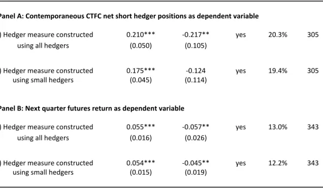
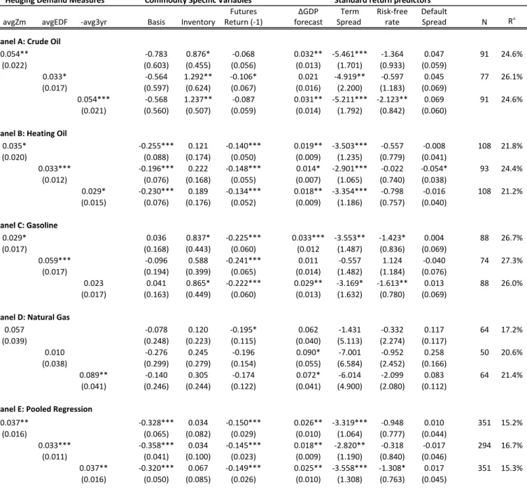
We verify that our results are driven by changes in producer hedging demand in a number of ways. First, we employ a “matching” approach. In particular, we separate the sample of producers into those firms that hedge commodity price exposure using derivatives (identified by their FAS 133 disclosures between 1998-2006), versus those that do not hedge. We show that our results are drivenonly by measures of aggregate hedging demand derived from thefirms that hedge. Second, we account for the possibility that default risk of commodity producers may be related to business-cycle conditions that also drive risk premiums. In particular, we employ controls in our forecasting regressions, in the form of variables commonly employed to predict the equity premium, such as changes in forecasts of GDP growth, the risk-free rate, the term spread, and the aggregate default spread, and confirm that our results are unaffected by the introduction of these controls. Third, from the set of commodityfirms that are included in our Crude Oil measures, we separate out pure play refiners from those that extract (or extract and refine) the commodity. Since refiners use crude (2007)). Fehle and Tsyplakov (2005) argue, both theoretically and empirically, thatfirms hedge more actively when default risk is higher.

2

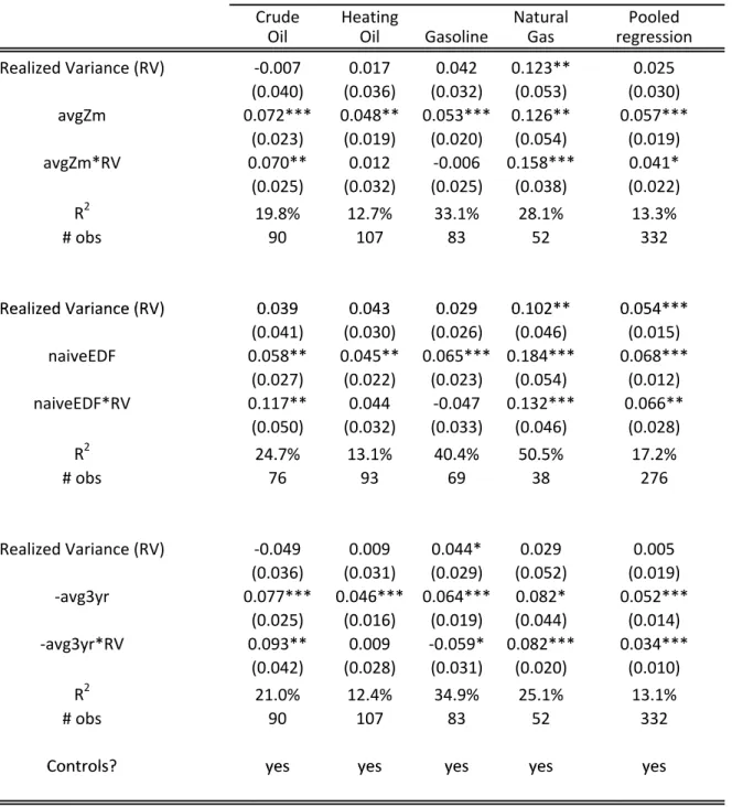
oil as an input, their hedging demand is likely to be in the opposite direction to that of producers — we verify this differential effect in the data. Finally, we employ controls that are commodity specific, such as the basis, inventory, lagged futures return, and the realized variance of futures returns in our specifications. This is to control for the possibility that producer default risk - an endogenous variable - may also be related to supply uncertainty, in the form of the likelihood of inventory stock-outs or other production shocks. Our model predicts that such supply uncertainty is related to the variance of the commodity price, but that increases in producer risk aversion should have effects as outlined earlier, even after controlling for this effect. The empirics confirm that default risk, our proxy for producer risk aversion, continues to explain futures risk premia after the introduction of these controls, indeed, there is an interactive effect of this predictive power with realized futures return variance as predicted by the model. To summarize, our model implies that limits to arbitrage generate limits to hedging for firms in the real economy. Consequently, factors that capture time-variation in such limits have predictive power for asset prices and affect outcomes in underlying product markets (spot prices and inventories). Our empirical results are consistent with the implications of the model and robust to a number of alternative explanations.

The remainder of the introduction relates our paper to the literature. Section 2 introduces our model. Section 3 presents our empirical strategy. Section 4 establishes the link between the hedging demand of commodity producers and measures of their default risk at the individual firm level. Section 5 discusses our main, aggregate empirical results. Section 6 concludes.

Related Literature. There are two classic views on the behavior of commodity forward and futures prices. TheTheory of Normal Backwardation (Keynes (1930)), states that speculators, who take the long side of a commodity futures position, require a risk premium for hedging the spot price exposure of producers (an early version of the “limits to arbitrage” argument). The risk premium on long forward positions is thus increasing in the amount of demand pressure from hedgers and should be related to observed hedger and speculator positions in the commodity forward markets. Carter, Rausser and Schmitz (1983), Chang (1985), Bessembinder (1992), and de Roon, Nijman, and Veld (2000) empirically link this “hedging pressure” to futures excess returns, the basis and the convenience yield, as evidence in support of this theory.

The Theory of Storage (Kaldor (1939), Working (1949), and Brennan (1958)), on the other hand, postulates that forward prices are driven by optimal inventory management. In particular, this theory introduces the notion of aconvenience yield to explain why anyone would hold inventory in periods in which spot prices are expected to decline. Tests of the theory include Fama and French (1987) and Ng and Pirrong (1994). In more recent work, Routledge, Seppi and Spatt (2000) introduce a forward market into the optimal inventory management model of Deaton and Laroque (1992) and show that time-varying convenience yields, consistent with those observed in the data, can arise even in the presence of risk-neutral agents.3

The two theories are not mutually exclusive. A time-varying risk premium on forwards is consistent with optimal inventory management if producers are not risk-neutral or face (say) bank-ruptcy costs; and speculator capital is not unlimited, as in our model. In the data, we find that hedgers are net short forwards on average, while speculators are net long, which indicates that producers do have hedging demands. In support of this view, Haushalter (2000, 2001) surveys 100 oil and gas producers over the 1992 to 1994 period andfinds that close to 50 percent of them hedge, in the amount of approximately a quarter of their production each year. In a recent paper, Gorton, Hayashi, and Rouwenhorst (2007) provide evidence that futures risk premia are related to inventory levels. Consistent with their findings, our model also predicts that inventory should forecast commodity futures returns. In our model, this results is driven by the interaction between capital-constrained speculators and producer hedging demand, proxied by measures of producer de-fault risk. Our empirical contribution is to identify that this dede-fault risk measure helps to explain commodity spot prices, risk premia, CFTC hedging pressure measures and inventory levels.

In closely related work, Hirshleifer (1988, 1989, 1990) considers the interaction between hedgers and arbitrageurs. In particular, Hirshleifer (1990) observes that in equilibrium there must be a friction to investing in commodity futures in order for hedging demand to affect prices and quantities. In our model, this friction arises due to limited movement of capital, motivated by the ‘limits to arbitrage’ literature, and hedging demand of producers, motivated by a principal-agent problem as the commodity firm is ultimately owned by the consumers. Furthermore, our analysis, unlike Hirshleifer’s, is also empirical. As a useful consequence, in addition to providing evidence for our model, we are able to confirm many of the propositions of Hirshleifer’s (1988, 1989, 1990) theoretical models, using a different approach than that in Bessembinder (1992). Another related paper is by Bessembinder and Lemmon (2002), who show that hedging demand affects spot and futures prices in electricity markets when producers are risk averse. They highlight that the absence of storage is what allows for predictable intertemporal variation in equilibrium prices. We show in this paper that the price impact can arise even in the presence of storage in the oil and gas markets. Finally, it has proven difficult to explain the unconditional risk premiums on commodity fu-tures using traditional asset pricing theory (see Jagannathan, (1985) for an earlier effort). Although conditional risk premiums on commodity futures do appear to be reliably non-zero (see Bessem-binder (1992)), BessemBessem-binder and Chan (1992) document that the forecastability of price changes in commodity futures is based on different asset pricing factors as compared to equity markets. Furthermore, in a recent paper, Tang and Xiong (2009) show that the correlation between com-modity and equity markets increases in the amount of speculator capital flowing to commodity markets. These results are consistent with our assumption of time-varying market segmentation between equity and commodity markets.

(1991), Schwartz (1997), Cassasus and Collin-Dufresne (2005)). General equilibrium models of commodity pricing include Cassasus, Collin-Dufresne, and Routledge (2009), and Johnson (2009).

2

The Model

We present a two-period model of commodity spot and futures price determination that includes optimal inventory management, as in Deaton and Laroque (1992), and hedging demand, similar to the models of Anderson and Danthine (1980, 1983) and Hirshleifer (1988, 1990). There are three types of agents in the model: (1) consumers, whose demand for the spot commodity along with the equilibrium supply determine the commodity spot price; (2) commodity producers, who manage profits by optimally managing their inventory and by hedging with commodity futures; and (3) speculators, whose demand for commodity futures, along with the futures hedging demand of producers, determine the commodity futures price.4

2.1

Consumption, Production and the Spot Price

Let commodity consumers’ inverse demand function be given by:

= µ   ¶1  (1)

whereis the commodity spot price,is the equilibrium commodity supply,is the consump-tion of other goods, andandare positive constants. This inverse demand function obtains if the representative agent has CES utility over the two goods (and) with an intratemporal elasticity of substitution equal to . In the Appendix, we argue that the main predictions of our model presented here are robust to a general equilibrium setting where this inverse demand function is derived endogenously. In the partial equilibrium setting considered here, however,  represents an exogenous demand shock, which we assume is lognormally distributed with [ln] =  and  [ln] =2. This shock captures changes in demand arising from sources such as technological changes in the production of substitutes and complements for the commodity, weather conditions, or other shocks that are not explicitly accounted for in the model.

Let aggregate inventory and production be denoted  and , respectively. Further, let  be the cost of storage; that is, individual producers can storeunits of the commodity at₋1yielding (1₋)units at, where  _∈(01) The commodity spot price is determined by market clearing, which demands that incoming aggregate inventory and current production,+ (1−)−1, equals

current consumption and outgoing inventory, +.

4_{We model consumers of the commodity as operating only in the spot market. This is an abstraction, which} does not correspond exactly with the evidence - for instance airlines have been known periodically to hedge their exposure to the price of jet fuel (by taking long positions in the futures market). In the empirical section, we show that our results are not affected by controlling for a measure of consumers’ hedging demand. Furthermore the CFTC data on hedger positions indicates that speculative capital (e.g., in hedge funds) has historically been allocated to long positions in commodity futures, indicating that the sign of net hedger demand for futures is consistent with our assumption.

2.2

Producers

There are an infinite number of commodity producing firms in the model, with mass normalized to one. Each individual manager acts competitively as a price taker. The timing of managers’ decisions in the model are as follows: In period 0, thefirm stores an amount  as inventory from its current supply, 0, and so period 0 profits are simply 0(0−). In period 0, the firm also

goes short a number of futures contracts, to be delivered in period1. In period1, thefirm sells its current inventory and production supply, honors its futures contracts and realizes a profit of

1((1−) +1) +( −1), where is the futures price and 1 is supply in period 1.5

We assume that managers of commodity producing firms are risk averse — they maximize the value of the firm subject to a penalty for the variance of next period’s earnings. This variance penalty generates hedging demand, and is a frequent assumption when modeling commodity pro-ducer behavior (for one recent example see Bessembinder and Lemmon (2002)).6 Writing Λ for the marginal rate of substitution (pricing kernel) of equity holders in the economy,7 and  for the risk-free rate, the managers’ objective function is:

max {} 0(0−) +[Λ{1((1−)+1) +( −1)}]  − ₂ [1((1−)+1) +( −1)] subject to: _≥0 (2)

The first order condition with respect to inventory holdingyields:

∗(1₋) = (1−)[Λ1]−0+ (1₋)2_ −

1+ (3)

whereis the Lagrange multiplier on the inventory constraint and_2 is the variance of the period1 spot price. As can be seen from Equation (3), managers use inventories to smooth demand shock. If, however, the current demand shock is sufficiently high, an inventory stock-out occurs (i.e., 0), and current spot prices can rise above expected future spot prices. In such a circumstance, firms

5_{Note that the production schedule,}

0 and1, is assumed to be pre-determined. The implicit assumption, which

creates a role for inventory management, is that it is prohibitively costly to change production in the short-run. 6_{The literature on corporate hedging provides several justifications for this modeling choice. Hedging demand} could result from managers being underdiversified, as in Amihud and Lev (1981) and Stulz (1984), or better informed about the risks faced by the firm (Breeden and Viswanathan (1990), and DeMarzo and Duffie (1995)). Managers could also be averse to variance on account of private costs suffered upon distress, as documented by Gilson (1989) for example, or thefirm may face deadweight costs offinancial distress, as argued by Smith and Stulz (1985). Aversion to earnings volatility can also be generated from costs of externalfinancing as in Froot, Scharfstein, and Stein (1993).

7

The setup implicitly assumes that the equity-holders cannot write a complete contract with the managers, on account of (for instance) incentive reasons as in Holmstrom (1979).

wish to have negative inventory, but cannot. Thus, a convenience yield for holding the spot arises, as those who hold the spot in the event of a stock-out get to sell at a temporarily high price. This is the Theory of Storage aspect of our model.8 Importantly, inventory is increasing in the amount hedged in the futures market,. That is, hedging allows the producer to hold more inventory as it reduces the amount of earnings variance that the producer would otherwise be exposed to. Thus, the futures market provides an important venue for risk sharing.

Thefirst order condition for the number of futures contracts that the producer goes short is:

∗_ =∗(1₋) +1−

[Λ(1−)] _2

 (4)

Note that if the futures price is such that[Λ(1₋)] = 0, there are no gains or costs to equity holders of the manager’s hedging activity in terms of expected, risk adjusted profits. The producer will therefore simply minimize the variance of period 1 profits by hedging fully. In this case, the manager’s optimal hedging strategy is independent of the degree of managerial risk aversion. This is a familiar result that arises by no-arbitrage in frictionless complete markets.

If, however, the futures price is lower than what is considered fair from the equity-holders’ perspective (i.e.,[Λ(1₋)]0), it is optimal for the producer to increase the expected profits by entering a long speculative futures position after having fully hedged the period 1 supply. In other words, in this situation, the hedge is costly due to perceived mispricing in the commodity market, and it is no longer optimal to hedge the period1price exposure fully. This entails shorting fewer futures contracts. Note that an increase in the manager’s risk aversion  decreases this implicit speculative futures position, all else equal.

The Basis. The futures basis is defined as:

_≡ 0− 0

=₋+

1₋ (5)

where  is the convenience yield. Combining the first order conditions of the firm (Equations (3) and (4)), the convenience yield is given by:

= 

0

1 +

1₋ (6)

The convenience yield can only differ from zero if the shadow price of the inventory constraint () is positive. In this case, the expected future spot price is low relative to the current spot price, and this results in the futures price also being low relative to the current spot price.

8_{In a multi-period setting, a convenience yield of holding the spot arises in these models even if there is no actual} stock-out, but as long as there is a positiveprobability of a stock-out (see Routledge, Seppi, and Spatt (2000)).

The basis is not a good measure of the futures risk premium when inventories are positive. Producers in the model can obtain exposure to future commodity prices in one of two ways — either by going long a futures contract, or by holding inventory. In equilibrium, the marginal payofffrom these strategies must coincide. Thus, producers managing inventory enforce a common component in the payoffto holding the spot and holding the futures, with offsetting impacts on the basis. This prediction of the model is borne out in our empirical results, and is consistent with thefindings of Fama and French (1987).

2.3

Speculators

Speculators take the long positions that offset producers’ naturally short positions, and allow the market to clear. We assume that these speculators are specialized investment management com-panies, with superior investment ability in the commodity futures market (e.g., commodity hedge funds and investment bank commodity trading desks). As a consequence of this superior invest-ment technology, investors in otherfinancial assets (the equity-holders) only invest in commodity markets by delegating their investments to these specialized funds. As in Berk and Green (2004), the managers of these funds extract all the surplus of this activity and the outside investors only get their fair risk compensation. The payoffto the fund manager per long futures contract is therefore

[Λ(1−)], making the net present value for equity-holders of investing in a commodity fund

zero, as dictated by no-arbitrage.

The commodity fund managers are assumed to be risk-neutral, but they are subject to capital constraints. These constraints could arise from costs of leverage such as margin requirements, as well as from value-at-risk (VaR) limits. We model these capital constraints as proportional to the variance of the fund’s position, in the spirit of a VaR constraint, as in Danielsson, Shin, and Zigrand (2008).9 _{Commodity funds are assumed to behave competitively, and we assume the existence of a} representative fund with objective function:

max  [Λ(1−)]−  2  [(1−)] (7) ⇓ ∗_ = [Λ(1−)] 2  (8)

whereis the severity of the capital constraint, andis the aggregate number oflong speculator

9_{Such a constraint is also assumed by Etula (2009) whofinds empirical evidence to support the role of speculator} capital constraints in commodity futures pricing. Gromb and Vayanos (2002) show in an equilibrium setting that arbitrageurs, facing constraints akin to the one we assume in this paper, will exploit but not fully correct relative mispricing between the same asset traded in otherwise segmented markets. Motivating such constraints on speculators, He and Xiong (2008) show that narrow investment mandates and capital immobility are natural outcomes of an optimal contract in the presence of unobservable effort on the part of the investment manager.

futures positions. If commodity funds were not subject to any constraints (i.e.,= 0), the market clearing futures price would be the same as that which would prevail if markets were frictionless; i.e., such that[Λ[(1−)] = 0. In this case, the producers would simply hedge fully, as discussed

previously, and the futures risk premium would be independent of the level of managerial risk aversion. With    0, however, the equilibrium futures price will in general not satisfy the usual relation, [Λ(1−)] = 0, as the risk-adjustment implicit in the speculators’ objective

function is different from that of the equity-holders.

2.4

Equilibrium

The futures contracts are in zero net supply and therefore=, in equilibrium. From equations (4) and (8) we obtain:

[Λ(1₋)] = 

+

2_1 (9)

where the variance of the spot price is 2_{ ≡}2−₁2 ³

()2₋1 ´

2+()2, and where period1 supply is1 =∗(1₋) +1. From the expression for the basis, (0₋)1+₁₋_ =. We have that:

[Λ1(∗)]−(0(∗)−(∗))(1−) =  + 1(∗)1−2 (10) where  _≡ 2 ³ ()2 ₋1 ´

2+()2. Equation (10) implicitly gives the solution for ∗. Since

 = (0(∗)−(∗))1+₁₋_, the equilibrium supply of short futures contracts can be found using

equation (4).

2.5

Model Predictions

Equation (9) can be rewritten in terms of the futures risk premium. In particular, defining  =  as the standard deviation of the futures return, 1_−, we have that:

 ∙ 1−  ¸ =₋(1 +)(Λ 1)(Λ) +  + (1 +)_2 1 (11)

Thefirst term on the right hand side is the usual risk adjustment term due to covariance with the equity-holders’ pricing kernel. However, the the producers and the speculators are the marginal investors in this market, rather than the equity-holders. The second term, which arises due to the combination of limits to arbitrage and producer hedging demand, has four components:  1, the

forward dollar value of the hedging demand,_2, the variance of the futures return,, producers’ risk aversion, and , speculator risk aversion. Note that Equation (11) holds for any consumer

preferences (inverse demand functions).10

Comparative Statics. We are interested in comparative statics with respect to producers’ propensity to hedge, (which we refer to henceforth as producers’fundamental hedging demand), and the degree of the capital constraint on speculators,. The proof of the following Proposition is relegated to the Appendix, and we only give the economic intuition for the results in this section.

Proposition 1 The futures risk premium and the expected spot price return are increasing in producers fundamental hedging demand, :

  [1−]  0 and   [1−0] 0 0 (12)

where the latter only holds if there is not a stock-out. In the case of a stock-out, _ 

[1−0] 0 = 0.

The futures risk premium and the expected spot price return are increasing in the severity of speculators’ capital constraints, :

  [1₋]  0 and   [1₋0] 0 0 (13)

where the latter only holds if there is not a stock-out. In the case of a stock-out, _ 

[1−0] 0 = 0.

The optimal inventory is decreasing in both producer and speculator hedging demand, unless there is a stock-out.

The intuition for these results is as follows. When producers’ fundamental hedging demand () increases, the manager’s sensitivity to the risk of holding unhedged inventory increases. In response to this, the manager reduces inventory and increases the proportion of future supply that is hedged. The former means that more of the commodity is sold on the spot market, which depresses current spot prices and raises future spot prices. The latter leads to a higher variance-adjusted demand for short futures contracts, which is accommodated by increasing the futures risk premium. An increase in speculator capital constraints,, has similar effect. The cost of hedging now increases as the speculators require a higher compensation per unit of risk. The direct effect of this is to decrease the number of short futures positions. However, this leaves the producer more exposed to 1 0_{Since producer hedging demand and limits to arbitrage both affect the optimal supply (inventory) of the} com-modity, the volatility of futures returns is also affected, meaning that the frictions assumed in the commodity market also show up in the standard risk adjustment (the covariance term). Thus, there is a component of the futures risk premium that originates from limits to arbitrage and hedging demand that cannot be separately observed from the standard risk adjustment. Symmetrically, if the volatility and mean of the demand shocks change, this is reflected in the volatility of the futures return which also shows up in the futures risk premium term due to hedging demand and limits to arbitrage. In the Appendix, we further discuss the interaction between the frictions proposed here and the standard risk adjustment in the context of a general equilibrium model where the pricing kernel and the inverse demand function are derived endogenously.

period1spot price risk, and to mitigate this effect, optimal inventory also decreases. In a stock-out, the inventory is constant (at zero) and consequently so are the expected spot price and its variance. In that case, the only effect of an increase in producer (or speculator) risk aversion is the direct effect on the futures risk premium, as the marginal cost of hedging increases.

To evaluate the likely magnitudes of the effect of the model’s frictions and to illustrate the model results, we calibrate the model using key moments of the data: in particular, the volatility of the commodity futures returns, commodity expenditure relative to aggregate endowment (GDP) and aggregate endowment growth, as well as the mean and volatility of the equity market pricing kernel. The details of the calibration are given in the Appendix.

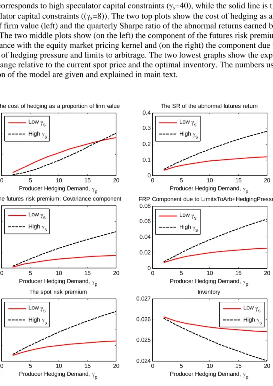
The severity of the model’s frictions are increasing in the variance aversion of producers and speculators,  and . The variation in these quantities is shown in the two top graphs of Figure 1 as the producers’ cost of hedging and the Sharpe ratio earned by speculators, where  is on the horizontal axis and  is shown as a dashed line for high speculator risk aversion and a solid line for low speculator risk aversion. The remainder of the plots in Figure 1 shows that the spot and futures risk premiums are indeed increasing in producer and speculator risk aversion, while inventory is decreasing. The calibration implies economically significant variation in both spot and futures risk premiums. In particular, for high speculator risk aversion (corresponding to their earning a quarterly Sharpe ratio of about025) and high hedging demand (corresponding to a loss of about08%offirm value due to hedging), the abnormal quarterly futures risk premium is about 6%, whereas for low producer hedging demand and speculator risk aversion (Sharpe ratio of about 005and loss from hedging of about01%of firm value), the abnormal futures risk premium is less than1%. At the same time, the impact on inventory is about a1%to9%change in the level. The effect on expected percentage spot price changes is about the same as for the futures, since the cost of carry relation holds when there is no stock-out. In sum, reasonable levels of the costs of hedging and required risk compensation leads to economically significant abnormal returns in the futures market, and concomitant changes in inventory and spot prices.

Figure 1also illustrates an intuitive interaction between speculator risk tolerance and producer hedging demand. In particular, the response of the abnormal futures risk premium to changes in producer hedging demand is smaller when speculator risk tolerance is high. These are times when speculators are willing to meet the hedging demand of producers with small price concessions. If, conversely, speculators are more risk averse, the price concession required to meet an additional unit of hedging demand is high.

3

Empirical Strategy

In our empirical analysis we test the main predictions of the model, as laid out in Proposition 1. To do so, we need proxies for  and  - the fundamental hedging demand and risk appetite of

producers and speculators, respectively. Clearly, from Equation (11), to identify time-variation in the futures risk premium from hedging pressure and limits to speculative capital, we must control for the covariance of the futures return with the equity pricing kernel. We therefore apply a substantial set of controls and robustness checks in the empirical analysis in order to establish that ourfindings arise on account of producer hedging demand and limited arbitrage capital.

3.1

Commodity Producer Sample

To construct proxies for fundamental producer hedging demand, we employ data on commodity producing firms’ accounting and stock returns from the CRSP-Compustat database. The use of Compustat data limits the study to the oil and gas markets as these are the only commodity markets where there is a large enough set of producer firms to create a reliable time-series of aggregate commodity sector producer hedging demand. Our empirical analysis thus focuses on four commodities: crude oil, heating oil, gasoline, and natural gas. The full sample of producers includes all firms with SIC codes 1310 and 1311 (Petroleum Refiners) and 2910 and 2911 (Crude Petroleum and Gas Extraction).11 _{The total sample of producers consists of 525firms with quarterly} data going back to 1974 for some firms. We also use data on firms’ explicitly disclosed hedging activities from accounting statements available in the EDGAR database from 1998 to 2006.

3.2

Proxying for Fundamental Hedging Demand

“The amount of production we hedge is driven by the amount of debt on our consolidated balance sheet and the level of capital commitments we have in place.”

- St. Mary Land & Exploration Co. in their 10-K filing for 2006.

In the model, we refer to the variance aversion of the producers,, as producers’ fundamental hedging demand. In the empirical analysis, we propose that variation in the aggregate level of can be proxied for, using measures of aggregate default risk for the producers of the commodity. There are both empirical and theoretical motivations for this choice, which we discuss below. In addition, we show in the following section that the available micro-evidence of individual producer hedging behavior in our sample supports this assumption.

The driver of hedging demand that we focus on is managerial aversion to distress and default. In particular, we postulate that managers act in an increasingly risk averse manner as the likelihood of distress and default increases. Amihud and Lev (1981) and Stulz (1984) propose general aversion of managers to variance of cashflows as a driver of hedging demand, the rationale being that while 1 1_{These SIC classifications, however, are rather coarse: firms designated as “Petroleum Refiners” (e.g., Exxon)} often also engage in extraction, and vice versa. In our robustness checks below, we separate out pure play refiners (as identified from their annual statements) fromfirms that engage in production, and separately evaluate the effects of default risk measures from each of these groups.

shareholders can diversify acrossfirms in capital markets, managers are significantly exposed to their

firms’ cash-flow risk due to incentive compensation as well as investments in firm-specific human capital. Empirical evidence has demonstrated that managerial turnover is indeed higher in firms with higher leverage and deteriorating performance: e.g., Coughlan and Schmidt (1985), Warner et al. (1988) and Weisbach (1988) provide evidence that top management turnover is predicted by declining stock market performance. Gilson (1989) refines this evidence, and examines the role of defaults and leverage. He first finds that management turnover is more likely following poor stock-market performance, and that firms that are highly leveraged or in default on their debt experience higher top management turnover than their counterparts. Gilson further documents that following their resignation from firms in default, managers are not subsequently employed by another exchange-listed firm for at least three years - consistent with managers experiencing large personal costs when their firms default. Finally, Haushalter (2000, 2001) in a survey of one hundred oil and gas firms over the 1992 to 1994 period, uncovers that their propensity to hedge is highly correlated with theirfinancing policies as well as their level of assets in place. In particular, he finds that the oil and gas producers in his sample that use more debt financing also hedge a greater fraction of their production, and he interprets this result as evidence that companies hedge to reduce the likelihood offinancial distress.

Given this theoretical and empirical motivation, we employ both balance-sheet and market-based measures of default risk as our empirical proxies for the cost of externalfinance. The balance-sheet based measure we employ is the Zmijewski (1984) score. This measure is positively related to default risk and is a variant of Altman’s (1968) Z-score, and the methodology employed to calculate the Zmijewski-score was developed by identifying the firm-level balance-sheet variables that help to “discriminate” whether afirm is likely to default or not. The market-based measures we employ arefirst (following Gilson (1989)), the rolling three-year average stock return of commodity producers, and second, the naive expected default frequency (or naive EDF) computed by Bharath and Shumway (2008).

Each firm’s Zmijewski-score is calculated as:

-= ₋43₋45_∗  + 57_∗  

−0004_∗ (14)

Eachfirm’s rolling three-year average stock return, writingfor the cum-dividend stock return for a firmcalculated at the end of month , is calculated as:

  = 1 36 35 X =0 ln(1 +−) (15)

Finally, we obtain each firm’s naive EDF. The EDF from the KMV-Merton model is computed using the formula:

 =Φ µ − µ ln( ) + (₋052_)  √  ¶¶ (16) where  is the total market value of the firm,  is the face value of the firm’s debt,  is the volatility of the firm’s value,  is an estimate of the expected annual return of the firm’s assets, and  is the time period (in this case, one year). Bharath and Shumway (2008) compute a ‘naive’ estimate of the EDF, employing certain assumptions about the variable used as inputs into the formula above. We use their estimates in our empirical analysis.12 Of the set of 525 firms, we have naive EDF estimates for 435firms.

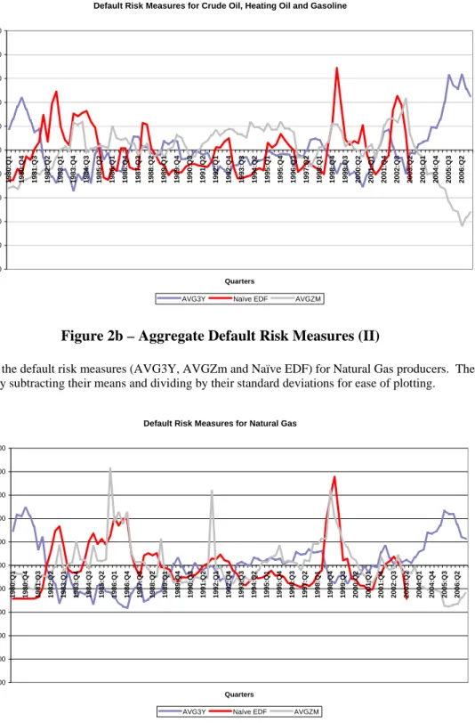
In the next section, we first confirm Haushalter’s (2000, 2001) results in our sample offirms — i.e., that our default risk measures are indeed related to individual producerfirms’ hedging activity. We then aggregate thesefirm-specific measures within each commodity sector to obtain aggregate measures of fundamental producer hedging demand, which are used to test the pricing implications of the model. To arrive at these aggregate measures of producer’s hedging demand, we construct an equal-weighted Zmijewski-score, 3-year lagged stock returns, and Naive EDF from the producers in each commodity sector. While our sample of firms goes back until 1974, the number offirms in any given quarter varies with data availability at each point in time. There are, however, always more than 10 firms underlying the aggregate hedging measure in any given quarter. Figures 2

and2show the resulting time-series of aggregate Zmijewski-score, 3-year lagged return, and Naive EDF for the Crude Oil, Heating Oil, and Gasoline sectors, as well as for the Natural Gas sector. For ease of comparison, the series have been normalized to have zero mean and unit variance. All the measures are persistent and stationary (the latter is confirmed in unreported unit root tests for all the measures). As expected, the aggregate Zmijewski-scores and Naive EDF’s are positively correlated, while the aggregate 3-year producer lagged stock return measure is negatively correlated with these measures. Table2reports the mean, standard deviation and quarterly autocorrelation of the aggregate hedging measures. The reason that these summary statistics are different for Crude Oil, Heating Oil, and Gasoline is that the futures returns data are of different sample sizes across the commodities.

4

Producers’ Hedging Behavior

While the main tests in the paper concern the relationship between spot and futures commodity prices and the commodity sector’saggregate fundamental hedging demand, wefirst investigate the available micro evidence of producer hedging behavior. Haushalter (2000, 2001) provides useful evidence of the cross-sectional determinants of hedging behavior among oil and gas firms, but his

1 2

evidence pertains to a smaller sample than ours, over the period from 1992 to 1994.13 A natural question for our purposes is to what extent the oil and natural gas producing firms in our sample actually do engage in hedging activity, and if so, in which derivative instruments and using what strategies. In this section, we use the publicly available data fromfirm accounting statements in the EDGAR database to ascertain the extent and nature of individual commodity producer hedging behavior.

4.1

Summary of Producer Hedging Behavior

The EDGAR database has available quarterly or annual statements for 231 of the 525 firms in the sample. In part, the smaller EDGAR sample is due to the fact that derivative positions are only reported in accounting statements, in our sample, from 1998 onwards.14 We determine whether or not each firm uses derivatives for hedging commodity price exposure by reading at least two quarterly or annual reports perfirm. Panel A in Table 1shows that out of the 231firms, there are 172 that explicitly state that they use commodity derivatives, 20 that explicitly state that they do not use commodity derivatives, and 39 that don’t mention any use of derivatives. Of the 172firms that use commodity derivatives, Panel B shows that 146 explicitly state that they use derivatives only for hedging purposes, while 16 firms say they both hedge and speculate. For the remaining 10 firms, we cannot tell. In sum, 74% of the producers in the EDGAR sample state that they use commodity derivatives, while a maximum of 26% of the firms do not use commodity derivatives. Of thefirms that use derivatives, 85% are, by their own admission, pure hedgers.

Panel C of Table1shows the instruments thefirms use and their relative proportions. Forwards and futures are used in 29% of the firms, while swaps are used by 52% of the firms. Options and strategies, such as put and call spreads and collars, are used by 20% and 33% of the firms, respectively. Most options positions are not strong volatility bets. In particular, low-cost collars that are long out-of-the-money put and short out-of-the-money calls are the most common option strategy for producers — a position that is very similar to a short futures position. Thus, derivative hedging strategies that are linear, or close to linear, in the underlying are by far the most common. We focus on short-term commodity futures - the most liquid derivative instruments in the commodity markets - in our empirical analysis. However, a considerable fraction of the hedging 1 3_{Another notable study offirm-level hedging behavior in commodities is Tufano (1996), who relies on proprietary} data from gold miningfirms.

1 4_{Since the introduction of Financial Accounting Standards Board’s 133 regulation (Accounting for Derivative} Instruments and Hedging Activities), effective for fiscal years beginning after June 15, 2000, firms are required to measure all financial assets and liabilities on company balance sheets at fair value. In particular, hedging and derivative activities are usually disclosed in two places. Risk exposures and the accounting policy relating to the use of derivatives are included in “Market Risk Information.” Any unusual impact on earnings resulting from accounting for derivatives should be explained in the “Results of Operations.” Additionally, a further discussion of risk management activity is provided in a footnote disclosure titled “Risk Management Activities & Derivative Financial Instruments.” Somefirms, however, provided some information on derivative positions also before this date.

is done with swaps, which are provided by banks over-the-counter, and often are longer term. On the one hand, this indicates that a significant proportion of producer’s hedging is done outside the futures markets that we consider. On the other hand, banks in turn hedge their aggregate net exposure in the underlying futures market and in the most liquid contracts. For instance, it is common to hedge long-term exposure by rolling over short-term contracts (e.g., Metallgesellschaft). A similar argument can be made for the net commodity option imbalance held by banks in the aggregate. Therefore, producers’ aggregate net hedging pressure is likely to be reflected in trades in the underlying short-term futures market.

4.2

The Time-Series Behavior of Producer Hedging

Information about hedging positions from accounting statements could potentially be used directly to assess the impact of time-varying producer hedging demand on commodity returns. However, there are significant data limitations for such use. First, FAS 133 requires thefirms to report mark-to-market values of derivative positions, which are not directly informative about underlying price exposure. There is no agreed upon reporting standard or requirement for providing information on effective price exposure for eachfirm’s derivative positions, which leads to either non-reporting, or very different reporting of such information. For instance, firms sometimes report notional outstanding or number of barrels underlying a contract, but not the direction of the position or the actual derivative instruments and contracts used, the 5%-, 10%-, or 20%-delta with respect to the underlying, or Value-at-Risk measures (again sometimes without mention of direction of hedge). We went throughall the quarterly and annual reports available for the firms with SIC codes 2910 and 2911 (50firms) in the EDGAR database to attempt to extract (a) whether thefirms were long or short the underlying, and (b) the extent of exposure in each quarter or year as measured by sensitivity to price changes in the underlying commodity futures price (i.e., a measure of Delta).

Panel D in Table 1 reports that of the 34 firms with these SIC codes that we could find in EDGAR, only 19 (56%) gave information about the direction of the hedge (long or short the underlying). Of these, 80%, on average, of the firm-date observations were short the underlying commodity. Since commodity producers are naturally long the commodity, one would expect that the producers’ derivative hedge positions are always short the underlying. However, there are complicating factors. First, somefirms do take speculative positions. Second, there are cases where hedging demand could manifest itself in long positions in the futures market. For instance, a pure refiner may have an incentive to go long crude oil futures to hedge its input costs, but short, say gasoline futures to hedge its production. This suggests that it might be fruitful to separate producers and producer refiners (such as Marathon Oil) from pure refiners (such as Frontier Oil) in the analysis, and we do so as a robustness check.

Of the 19 firms that reported whether they were long or short in the futures markets, we could only extract a reliable, and relatively long, time-series of derivative position exposure to the

under-lying commodity price for 4 firms: Marathon Oil, Hess Corporation, Valero Energy Corporation, and Frontier Oil Corporation. Consequently, the data is not rich enough to provide a measure of aggregate producer hedging positions based on direct (self-reported) observations of producers’ futures hedging demand, even for the relatively short period for which EDGAR data is available. Nevertheless, we show the relationship between the time series of hedging behavior and default risk for the 4firms for which we were able to extract this information. This represents an interest-ing insight into the time-series variation in hedginterest-ing, which complements existinterest-ing analyses (such as Haushalter (2000, 2001)) of the cross-sectional relation between hedging behavior and default risk measures.

4.3

Observed Hedging Demand and Default Risk

From the quarterly and annual reports of these four firms, we extract a measure of each firm’s $1 delta exposure to the price of crude oil (i.e., how does the value of the company’s derivative position change if the price of the underlying increases by $1). This measure of eachfirm’s hedging position is constructed from, for instance, value-at-risk numbers that are provided in the reports by assuming log-normal price movements and using the historical mean and volatility from the respective commodity futures returns. In other cases, firms report delta’s based on 5%, 10% and 20% moves in the underlying price, which are then used to construct the $1 delta number as a measure of hedging demand.

We next compare the time-series of each of the firms’ commodity derivatives hedging demand to each firm’s Zmijewski-score and 3-year lagged stock return throughout the EDGAR sample. There are too few observations per firm to compare with the naive-EDF scores, which is only provided to us until the end of 2003. Figure 3 shows the negative of the imputed delta and the Zmijewski-score for each of the four companies. Both variables are normalized to have mean zero and unit variance. The figure shows that there is a strong, positive correlation between the level of default risk, as measured by the Zmijewski-score and the amount of short exposure to crude oil using derivative positions for Marathon Oil, Hess Corp., and Valero Energy Corp. For Frontier Oil Corp., the hedging activity is strongly negatively correlated with the Zmijewski-score. The same pattern can be seen in Figure3, where eachfirm’s hedging activity is plotted against the negative of its 3-year average stock returns. Marathon Oil and Hess both extract and refine oil and so it is natural that as default risk and hedging demand increases, these firms increase their short crude oil positions. Valero, however, is a pure refining company that one might argue should go more long crude oil as default risk increases. This does not happen, however, because Valero in fact holds inventory of its input, crude oil, as well as for refined products. This was inferred by reading Valero’s quarterly reports, and is anecdotally quite a common happenstance for refiners. Thus, an increase in the demand for hedging leads to increasing hedge of both the input and output good inventories. Frontier Oil, however, behaves more as one might naively expect of a refiner, as the

company does not hold significant crude inventory in this sample, and decreases its short crude positions as default risk increases. Finally, as a check that the proxies used capture default risk in our sample, Figure3shows the time-series relation between Valero’s 5-year CDS spread (obtained from Markit) and its short crude oil hedging. Valero is the only of thesefirms where CDS data was available to us. Again, we see a strong relation between hedging and default risk.

In sum, in these four firms, which constituted the best sample available in EDGAR of the producerfirms, it is clear that hedging activity is time-varying, and related to the proposed proxies for fundamental hedging demand. However, the graphs highlight that one must take care when inferring expected hedging activity from whether afirm is involved only with extraction, extraction and refining, or purely refining. Essentially, all firms are to some extent naturally long crude oil, but for pure refiners, this is likely less true than for companies that engage in both extraction as well as refining - echoing the analysis in Ederington and Lee (2002).

We now turn to our analysis of theaggregate relationships between our proxies for fundamental hedging demand, spot returns and futures risk premia in the oil and gas markets. We will, however, use the non-hedgingfirms identified in the micro-analysis in this section and the separation between producers and refiners to perform robustness checks for our aggregate results to come.

5

Aggregate Empirical Analysis

In this section, we employ the aggregate measures of producer hedging demand, for which we reported summary statistics in the Data section, to test the empirical predictions of the model documented in Section2.

5.1

Commodity Futures and Spot Prices

Our commodity futures price data is for NYMEX contracts and is obtained from Datastream. The longest futures return sample period available in Datastream goes from the first quarter of 1980 until the fourth quarter of 2006 (108 quarters; crude oil).

To create the basis and returns measures, we follow the methodology of Gorton, Hayashi and Rouwenhorst (2007). We construct rolling commodity futures excess returns at the end of each month as the one-period price difference in the nearest to maturity contract that would not expire during the next month. That is, the excess return from the end of monthto the next is calculated as:

+1 − 

 (17)

where is the futures price at the end of monthon the nearest contract whose expiration date  is after the end of month+ 1, and+1 is the price of the same contract at the end of month + 1. The quarterly return is constructed as the product of the three monthly gross returns in the

quarter.

The futures basis is calculated for each commodity as (12₋1), where 1 is the nearest futures contract and 2 is the next nearest futures contract. Summary statistics about these quarterly measures are presented in Table2. Note that the means and medians of the basis in the table are computed using the raw data, while the standard deviation andfirst-order autocorrelation coefficient are computed using the deseasonalized basis, where the deseasonalized basis is simply the residual from a regression of the actual basis on four quarterly dummies. The basis is persistent across all commodities once seasonality has been accounted for.

Table2further shows that the excess returns are on average positive for all three commodities, ranging from25%to67%, with relatively large standard deviations (overall in excess of20%). As expected, the sample autocorrelations of excess returns on the futures are close to zero. The spot returns are defined using the nearest-to-expiration futures contract, again consistent with Gorton, Hayashi and Rouwenhorst (2007):

+1+2−+1 +1

 (18)

Again, the quarterly return is constructed by aggregating monthly returns as defined above. Note that the spot returns display negative autocorrelation, consistent with mean-reversion in the level of the spot price.

5.2

Inventory

For all four energy commodities, aggregate U.S. inventories are obtained from the Department of Energy’s Monthly Energy Review. For Crude Oil, we use the item: “U.S. crude oil ending stocks non-SPR, thousands of barrels.” For Heating Oil, we use the item: “U.S. total distillate stocks”. For Gasoline, we use: “U.S. total motor gasoline ending stocks, thousands of barrels.” Finally, for Natural Gas, we use: “U.S. total natural gas in underground storage (working gas), millions of cubic feet.” Following Gorton, Hayashi and Rouwenhorst (2007), we compute a measure of the discretionary level of aggregate inventory by subtracting a moving trend of inventory from the quarterly realized inventory (so as to avoid look-ahead bias). Quarterly trend inventory is created using a Hodrick-Prescott filter with the recommended smoothing parameter (1600). In all specifications that employ inventories, we also include quarterly dummy variables, to control for the strong seasonality present in inventories. Table 2 shows summary statistics of the resulting aggregate inventory measure, i.e., the cyclical component of inventory stocks, for the commodities. Once the seasonality in inventories is accounted for, the trend deviations in inventory are persistent.

5.3

Hedger Positions Data.

The Commodity Futures Trading Commission (CFTC) reports aggregate data on net “hedger” positions in a variety of commodity futures contracts. These data have been used in several papers that arrive at differing conclusions about their usefulness. For example, Gorton, Hayashi and Rouwenhorst (2007)find that this measure of hedger demand does not significantly forecast forward risk premiums, while De Roon, Nijman and Veld (2000)find that they hold some forecasting power for futures risk premia. The CFTC hedging classification has significant shortcomings; in particular, anyone that can reasonably argue that they have a cash position in the underlying can obtain a hedger classification. This includes consumers of the commodity, and more prominently, banks that have offsetting positions in the commodity (perhaps on account of holding a position in the swap market). The line between a hedge trade and a speculative trade, as defined by this measure, is therefore blurred. We note these issues with the measure as they may help explain why the forecasting power of hedging pressure for futures risk premia is debatable, while our measures of default risk do seem to explain futures risk premia. Nevertheless, we use the CFTC data as a check that our measures of producers’ hedging demand is in fact reflected in futures positions as noted by the CFTC.

The Hedger Net Positions data are obtained from Pinnacle Inc., which sources data directly from the Commodity Futures Trading Commission (CFTC). Classification into Hedgers, Speculators and Small traders is done by the CFTC, and the reported data are the total open positions, both short and long, of each of these trader types across all maturities of futures contracts. We measure the net position of all hedgers in each period as:

  =

( − ) ( −1+ −1)

 (19)

This normalization means that the net positions are measured relative to the aggregate open interest of hedgers in the previous quarter. Summary statistics on these data are shown in Table 2. First, the hedger positions are on average positive, which means investors classified as “hedgers” are on average short the commodity forwards. However, the standard deviations are relatively large, indicating that there are times when the CFTC classified “hedgers” are actually net long commodity futures contracts.

5.4

Aggregate Controls

In our empirical tests, we use controls to account for sources of risk premia that are not due to hedging pressure. In a standard asset pricing setting, time-varying aggregate risk aversion and/or aggregate risk can give rise to time-variation in excess returns. This is reflected in the pricing kernel,Λ, of equity-holders in the model. To capture this source of variation, therefore, we include

business cycle variables that have been shown to forecast excess asset returns in previous research. We include the Default Spread: the difference between the Baa and Aaa rated corporate bond yields, which proxies for aggregate default risk in the economy and has been shown to forecast excess returns on stocks and bonds (see, e.g., Fama and French (1989), and Jagannathan and Wang (1996)). Following Harrison and Yogo (2009), we also include the Term Spread, constructed as the difference between the yield on a 5-year zero-coupon T-bond and the yield on the 3-month T-bill. We do not include the aggregate dividend yield, as this variable has no forecasting power for commodity returns (results available on request). Finally, to account for time-varying expected commodity spot demand, we use a forecast of quarterly GDP growth, obtained from the Philadelphia Fed’s survey of professional forecasters.

5.5

Commodity Speci

fi

c Controls

We also include controls that are specific to each commodity. As emphasized in Gorton, Hayashi, and Rouwenhorst (2008), the cyclical level of inventory is related to the conditional volatility of the commodity price, and as such, the volatility of spot and futures returns. The basis is related to (the probability) of an inventory stock-out, and so is expected to have predictive power mainly for the spot return. When there is ample inventory, however, the basis is not expected to be informative about spot or futures returns, and so it should not drive out predictability that arises from producer hedging demand. The lagged futures return is included to capture autocorrelation in excess futures returns not captured by the other controls. A component of the measures of producer default risk will be related to lagged commodity returns (asfirm performance is related to commodity returns), and we want to ensure that the proxies for producer hedging demand are not simply capturing this autocorrelation in commodity returns. Finally, we include quarterly dummy variables in all the regressions as both the independent and many of the dependent variables in the regressions exhibit seasonalities.

5.6

Empirical Results

Before we test the predictions of the model with respect to the expected commodity futures and spot return, wefirst perform an additional check of the validity of the aggregate measures of producers’ fundamental hedging demand by relating them to the CFTC measures of aggregate net hedging demand. As previously explained, the aggregate CFTC data on hedger positions is noisy. However, a noisy measure of hedger positions should still contain information about the underlying true producer hedging demand.

5.6.1 CFTC Hedging Positions and Producer Hedging Demand

We construct the hedger net position variables from the CFTC data as the net short position, so we should expect a positive relation between the default risk and CFTC hedger positions. Table 3 reports the results of the regression:

   = + + (20)

where  denotes the relevant commodity (crude oil, heating oil, gasoline, or natural gas). The term "ControlVariables" is a catch-all term for the inclusion of the control variables described earlier, and “ ” denotes the average producer Zmijewski-score, the average producer Naive EDF, or the negative of the 3-year average producer stock returns (so as to make the expected regression coefficient, , positive in all specifications). In these regressions, both the left- and right-hand side variables are normalized to have unit variance, so the regression coefficients can be easily interpreted. Table 3 shows that 10 out of12 of the regression coefficients (0_{) are positive} and that half are positive and significant at the10% level or greater at the individual commodity level. The significance level is overall increasing in the number of observations available (Natural Gas and Gasoline have the fewest observations and largely insignificant coefficients). To alleviate issues regarding power, we present in the right-most column of Table 3 the -coefficients from pooled regressions across all commodities for all the default risk measures. In all three cases, the regression coefficient is positive and significant at the 5% level.15 _{Thus, the aggregate measures} of producer hedging demand are indeed significantly and positively related to the CFTC recorded aggregate "hedger" positions.

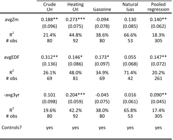
5.6.2 Commodity Futures Returns

Next, we evaluate the first part of Proposition 1, namely that increases in fundamental hedging demand are associated with higher futures risk premia. To do so, we run a standard forecasting regression for excess commodity futures return, using our default risk proxy for fundamental hedging demand. In particular, we regress quarterly (excess) futures returns on one quarter lagged measures of default risk and control variables:

+1= + ++1 (21)

wheredenotes the commodity and denotes time measured in quarters.

Table 4 shows the results of the above regression across the four commodities considered, as 1 5

Note that in all individual-commodity regressions in this paper, standard errors are constructed using the Newey-West (1987) method, which is robust to heteroskedasticity and autocorrelation of the error terms, and in all pooled regressions, we employ Rogers (1983, 1993) errors that are robust to heteroskedasticity, own and cross-autocorrelation and contemporaneous correlation across all commodities in each quarter.