Self-Aware Scheduling for Mixed-Criticality Component-Based Systems

Self-aware scheduling for

mixed-criticality component-based systems

Johannes Schlatow, Mischa M¨ostl and Rolf Ernst TU Braunschweig, IDA

{schlatow,moestl,ernst}@ida.ing.tu-bs.de

Abstract—A basic mixed-criticality requirement in real-time systems is temporal isolation, which ensures that applications receive a guaranteed (CPU) service and impose a bounded interference on other applications. Providing operating system support for temporal isolation is often inefficient, in terms of utilisation and achieved latencies, or complex and hard to implement or model correctly. Correct models are, however, a prerequisite when response times are bounded by formal analyses. We provide a novel approach to this challenge by applying self-aware computing methodologies that involve run-time monitoring to detect (and correct) model deviations of a budget-based scheduler.

I. INTRODUCTION

In Mixed-Criticality Systems (MCS), a processing platform hosts applications of different importance for the “mission” of a cyber-physical system. A high-critical application is typically developed with high quality standards in order to assure its correct operation. As this assurance does not hold for all system parts, such systems must employ the basic principle of isolating higher criticalities from any influence of lower-critical application. More precisely, criticality should be perceived as an attribute of a requirement, i.e. a system-level constraint, rather than an attribute of an application [1]. When it comes to (real-)time requirements, temporal isolation must thus be achieved. As recently stated by Lyons et al., “MCS require OS support for a form of temporal isolation, where (lower criticality) high-priority threads can preempt (highly critical) threads, but cannot monopolise the processor” [2]. Although static-priority scheduling provides temporal isolation from lower-priority threads, criticalities cannot be used as scheduling priorities in general. Similarly, fixed time slices are an inefficient solution for temporal isolation w.r.t. utilisation and latencies.

Unlike static mixed-criticality scheduling techniques [3] that are restricted to two criticalities and only provide guarantees for the highest criticality, we consider MCS from a more practical perspective. In these regards, scheduling policies such as sporadic-server scheduling have been proposed but turned out to be rather complex and hard to implement correctly [4], [5]. For real-time systems, there are two key properties: first, the correct (timely) operation of the application itself (guaranteed service) and, second, the bounded (temporal) interferencefrom other applications. The latter in particular is a prerequisite for bounding response times, e.g. by performing a model-based Worst-Case Response Time (WCRT) analysis,

which is the major requirement in real-time systems. However, models only capture abstract concepts and assumptions that may not exactly reflect the actual implementation of the ap-plications and the Operating System (OS). Particularly for low-criticality applications, abstractions and approximations are getting more prominent. Corner cases in regards to temporal isolation may furthermore only occur under certain load, with certain applications or with a particular system composition. Therefore, temporal isolation cannot be guaranteed (and sus-tained during the system’s life cycle) by WCRT analysis or by (operating-)system design alone. Instead, we propose a combined approach for providing temporal isolation, which is essential for MCS. By bringing the models into the run-time domain we enable the system to adapt to detected model changes, which is a basic principle of self-aware computing systems as we will explain in Section III.

Contributions:We suggest a budget-based scheduling with an event-based replenishment policy for basic temporal iso-lation. We augment this by run-time tracing and monitoring mechanisms to detect model deviations in the scheduling w.r.t. required budgets and scheduling overheads that result from inaccurate time accounting. By combining both techniques, we achieve self-aware scheduling. We implemented our tech-niques in a microkernel-based system.

Section II states the models that we take as a basis before we present our contributions in Section III. In Section IV, we summarise related work in the corresponding research fields. The evaluation of our approach and its implementation is given in Section V before we conclude with our final thoughts in Section VI.

II. SYSTEM MODEL

We base our implementation on the open-source Genode OS Framework [6]. This framework follows the microkernel approach and employs a strict decomposition of the system on application level, resulting in a service-oriented architecture in which separate components implement and provide services for other components. While decomposition can already deal with liveliness issues [7] that arise in mixed-critical systems, dependencies on the execution time or response time of other components remain [8] due to imperfect temporal isolation. Exposing these dependencies requires a timing model of the entire workload. In order to resolve these dependencies, M¨ostl et al. [8] suggest run-time enforcement mechanisms.

In this work, we distinguish between an application-centric timing model and a kernel-centric timing model. The former describes the interactions and dependencies between the activ-ities of communicating components, and serves as a basis for exposing (timing) dependencies between components as well as for determining scheduling priorities. The latter models how the kernel schedules the different schedulable entities.

When integrating mixed-critical systems, both models are essential. The application timing model provides all the information required for determining worst-case end-to-end latencies for particular processing chains and hence enables verification of application timing constraints. In contrast, the kernel timing model focuses on scheduling decisions and overheads, thereby abstracting the actual implementation and serves as a basis for configuring enforcement mechanisms.

This section summarises the models we apply on both levels and provides details and assumptions about the existing OS kernel implementation.

A. System composition

We consider component-based systems that follow the mi-crokernel approach. A component in such a system is spatially isolated, i.e. it has its own address space. Components can communicate with each other using client/server – i.e. Remote-Procedure Call (RPC) – or sender/receiver semantics. The communication policy follows the principle of least privilege such that access rights can be passed on a fine-grained level. Management of policy is typically performed by a separate component that delegates resources and access. In the scope of this work, we assume that components are single threaded.

B. Application timing model

In consequence of our system composition, the application timing model consists of communicating threads. From a functional perspective, thread communication is commonly modelled by sequence diagrams that show the activities of threads and their interactions. In a timing model, tasks reflect these activities and their precedence relations, which lead to task chains [9]. A task is activated by a stimulus, executes for a certain time and may emit a stimulus when it completes. A certain instance of a task’s execution is also referred to as a job. Due to the different communication semantics, we distinguish two types of precedence relations: Asynchronous

precedence means a task can be activated again right after its completion. For synchronous precedence (e.g. RPC), a task must wait for the completion of its successor before a new job can be executed. A task therefore resembles a sequence of code within a thread whereas precedence relations reflect communication between threads.

The OS performs scheduling on a per-threads basis, i.e. a thread not only delivers the code to be executed but also the scheduling parameter (e.g. priority or time slice). Hence, there is a dualism of threads as model entities as they not only reflect a temporal (scheduling) but also a spatial (shared resource) property: A thread performing a RPC blocks the address space of the callee such that all other callers (synchronous

predecessors) of the callee must wait for its completion before their RPC can be handled. The shared resource aspect of threads may lead to priority inversion, which is typically addressed by inheritance protocols [10], [11].

Note, that shaping (i.e. enforcement of execution times) on basis of the application timing model, would be rather complex and heavyweight as the kernel/scheduler is not aware of these model abstractions. It does not appear practical to match the application timing model with the scheduler’s native abstractions at run time. Furthermore, Schlatow and Ernst [12] showed that the run-time efficiency of a response-time analysis for complex task chains is not suitable for in-field application and hence not suitable for self-aware scheduling. In consequence, a simpler analysis approach is required that goes hand-in-hand with the implementation.

C. Kernel (timing) model

The section below summarises implementation details and assumptions about the kernel before we specify our kernel-timing model. The kernel implements RPCs and signals as inter-component communication mechanisms. These mecha-nisms directly resemble the client/server and sender/receiver communication schemes mentioned above. The kernel im-plements Symmetric Multiprocessing (SMP) with one kernel stack and one scheduler per core. Concurrent access to kernel objects is managed by a kernel lock which ensures that only one core at a time can reside in kernel. The kernel schedules the threads on each core based on the active scheduling contexts [2], [13]. A scheduling context has an execution budget and references the thread that currently executes in this context. This way, execution budgets can be passed between threads on RPCs, which effectively implements donationand

helping that are commonly used in microkernels [10] to mitigate priority inversion. As we do not want to go into the details of these mechanisms in the scope of this paper, we rather focus on the implications that these have on the application timing model.

1) Tasks with synchronous precedence (RPC) are executed within the same scheduling context (donation).

2) In case of helping, blocked tasks donate their scheduling context (e.g. priority, time slice) such that the waiting time is limited (no nested blocking).

Note that the definition and replenishment of the actual ex-ecution budgets is part of the scheduling policy. Similarly, the selection of scheduling contexts is also part of the scheduling policy (e.g. priority based, round robin).

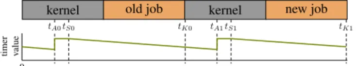
1) Time accounting: The kernel is implemented tickless, i.e. the scheduler uses a core-private timer in one-shot mode to perform time accounting and process timeouts based on the calculated OS time. Figure 1 and Figure 2 depict how the scheduler performs time accounting using the one-shot timer. More specifically, a switch from an old job to a new job is depicted, which involves the invocation of the kernel and scheduler. Such a switch can be caused by interrupts, CPU exceptions, syscalls or timer expirations. Note that the scheduler may select the same job again (old job = new job).

At timetA0 the scheduler reads the timer value to advance the OS time, processes timeouts and calculates the budget consumed by the current job. At time tS0, the scheduling decision was made and the timer is set to the next timeout (i.e. budget expiration) and started. Some time later, old job

is executing until tK0 where the kernel is entered again. Similarly, at tA1 the OS time is advanced bytA1−tS0 and the timer is set fornew job attS1.

kernel old job kernel new job

tS0

tA0 tK0 tA1tS1 tK1

0

timer value

Figure 1. Time accounting in case of interrupt, CPU exception or syscall.

kernel old job kernel new job

tS0

tA0 tK0 tA1tS1 tK1

0

timer value

Figure 2. Time accounting in case of timer expiration. We now want to have a more detailed look at how execution budgets are accounted in order to reveal possible inaccuracies. As long as the timer is running (decreasing), the passed time can be accounted as consumed execution budget of the current job no matter if the time was spent in kernel or user-level. More specifically, we definetS0/tS1 as the time at whichold

job/new jobis scheduled. Ideally, we want the time between tS1−tS0 being accounted to the execution ofold job.

However, as illustrated by Figure 1, the timer is halted betweentA1andtS1. In consequence, the budget ofold jobis subtracted bytA1−tS0, which effectively increases the budget ofold jobbytS1−tA1 for every preemption1. We denote this as preemption overhead.

Moreover, in case the timer runs to zero at any point between tK0 and tA1 as illustrated in Figure 2, the time betweentK0 andtS1 remains unaccounted in the worst case. This increases the budget ofold jobbytS1−tK0. As this may only happen if old jobconsumed all its execution budget, we denote this as budget expiration overhead.

Additionally, due to the kernel lock, in multi-core systems, kernel entry will be delayed if another core resides in kernel-mode. As long as the timer keeps running, this is accounted as consumed budget. If the timer expired, this kernel lock over-head must be considered as additional unaccounted budget.

We are aware that a careful kernel implementation would make use of an incrementing counter that never stops in order to eliminate the preemption overhead. However, such a timer is not available on all architectures or may rather be used for other purposes. Hence, in the scope of this work, we focused

1_{We denote interrupts, CPU exceptions and syscalls as preemptions}

irre-spective of whether new job is actually different from old job.

on dealing with such imperfect implementations by means of self-awareness.

2) Budget scheduling model: As was mentioned in the beginning of this section, we now define a kernel timing model. This model shall capture the scheduling behaviour w.r.t. inaccuracies and overheads of the execution budgets that are assigned to the scheduling contexts. More specifically, we are interested in a) the guaranteed service (in terms of CPU time) that a scheduling context will receive for a given execution budget, and b) the maximum interference that other scheduling contexts may experience. Note, that we do not distinguish between time spent in kernel- or user-level.

Definition 1: Theguaranteed servicefor a scheduling con-texts is calculated by the granted budget and a non-negative additive errorQper preemption:

service(s) =granted budget+ #preemptions·Q

Definition 2: Themaximum interferencefrom a scheduling context s is calculated by its granted budget, a non-negative additive error P per preemption and a non-negative additive errorE:

interference(s) =granted budget+ #preemptions·P+E

The errors Q and P are determined by lower resp. upper bounds for the preemption overhead. The error E combines upper bounds on the budget expiration and kernel lock over-head. These can be either derived analytically (by Worst-Case Execution Time (WCET) analysis) or determined by measure-ments as we do in Section V. As these measuremeasure-ments typically do not serve as sound upper bounds, we suggest a monitoring approach to detect model deviations in Section III-C2. Note, that we only consider additive errors and exclude multiplica-tive errors, i.e. errors that depend on the budget value. Our rationale is that multiplicative errors will be small enough in the typical time range (from hundreds of microseconds to a few seconds) so that they can be approximated by additive errors.

III. SELF-AWARE SCHEDULING

Before elaborating on our approach to self-aware schedul-ing, it is important to first have a look at howself-awarenessis defined in the literature. Lewis et al. [14] define self-awareness in computing systems based “on the idea of a conceptual component called a self-aware node”, which does not need to correspond to a physical (hardware, software) component:

“To be self-aware a node must:

• Possess information about its internal state (private self-awareness).

• Possess sufficient knowledge of its environment to deter-mine how it is perceived by other parts of the system (public self-awareness).” [14]

Lewis et al. also defineself-expressionas:

• “A node exhibits self-expression if it is able to assert its behaviour upon either itself or other nodes.

• This behaviour is based upon the node’s state, context, goals, values, objectives and constraints.” [14]

In these terms, self-expression denotes the (re)actions that a system performs based on the knowledge of its own state and its environment (self-awareness).

Note, that these definitions rather focus on functional as-pects (behaviour) of computing systems whereas we take a platform-centric view on these terms in the scope of this paper. More specifically, we suppose that the scheduling resembles the self-aware node and that its environment is perceived in form of the application timing model.

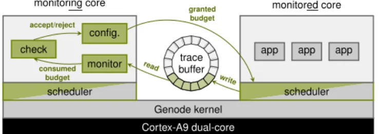
Cortex-A9 dual-core Genode kernel scheduler scheduler app app app check monitor config.

monitoring core monitored core

trace buffer write read consumed budget accept/reject granted budget

Figure 3. Architecture overview of our self-aware scheduling approach. Contributions are highlighted.

The following sections present our approach to self-aware scheduling, which comprises three building blocks: First, a shaping mechanism implements an enforcement of assumed execution-time budgets, which, on the one hand, provides service guarantees to the shaped thread and, on the other hand, limits the interference to other threads. Second, a tracing mechanism instruments the scheduler in order to make the scheduling behaviour observable and enable monitoring at user level. Third, monitoring is implemented as a user-level component that evaluates the traces as well as detects and corrects model deviations. Figure 3 provides an architectural overview of this approach.

A. Shaping: enforcement of execution-time budgets

In Section II-C, we modelled the budget-scheduling mecha-nism of the kernel which, in conjunction with a replenishment policy, builds our shaping mechanism. This section gives a more detailed account of our replenishment policy that is comparatively low in run-time overhead and complexity.

1) Background: Ideally, we would like to have a replen-ishment policy that follows the sporadic server scheduling concept [15]. This concept assumes that a consumed amount of budget is replenished after a time interval Rt after its consumption, i.e. in any time window of size Rt a thread is granted a constant budgetB. Hence, in real-time analysis, such a thread can be replaced by an analogous periodic task with period Rt and execution time B. In contrast, the deferrable

serverconcept assumes a periodic replenishment with a period Rt, i.e. every Rt the budget is reset to B no matter how much and when the budget was consumed. In consequence, the thread can receive a budget of up to2B in a time window of sizeRt, which renders real-time analysis conservative as the thread is guaranteed only a budget of B but it may consume up to2B in the worst case.

While deferrable server scheduling is simple to implement,

idealsporadic server scheduling cannot be implemented as it requires tracking an infinite number of (time-triggered) replen-ishments. Hence, in practice, the number of replenishments must be limited. At the same time, time resolution must be taken into account. A more practical definition of this concept is given by the POSIX sporadic server, which, however, is still complex and as shown by defects discovered and corrected later [4].

A general drawback of this concept is the replenishment fragmentation that results from it as every preemption will lead to a time-triggered replenishment of the consumed budget, thus causing a timeout (i.e. another preemption) afterRt. Of course, this can be counteracted at the cost of approximations (limiting the number of replenishments or the time resolution). Nevertheless, the more complex such an implementation is and the more corner cases it contains, the more effort must be spent for verification tasks such as real-time analysis and verification/certification of the implementation.

From the application perspective, the configuration of a sporadic server consists of setting an utilisation (single value) that allows the thread to be served fast enough and limits its interference on other threads. However, this does not quite match the application timing model introduced in Section II-B that we use to model application workload more accurately. This is due to the fact that a task/job resembles a certain sequence of code within a thread. Depending on input data and inter-thread communication, different job sequences (traces) can be observed, e.g. traces with a hyper-periodic sequence of execution times. There exists a large body of research looking at more exact digraph task models [16], [17] than the periodic task model. In the scope of this work, we use the execution time model (ET model) [18] that generalises such traces and that is comparatively low in complexity when it comes to implementation.

Definition 3: Theexecution time modelof a taskτiconsists of two functions(ET_i−, ET_i+)such that∀n∈_N+_:ET−

i (n) (resp.ET_i+(n)) is the best-case (resp. worst-case) cumulative execution time ofn consecutive instances. [18]

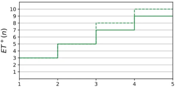
In other words, theET_i+(n)function bounds the execution time that can at most be seen from any sequence of n consecutive jobs of task τi. For instance, the WCET of τi is given by ET_i+(1) whereas two consecutive jobs of τi will not execute longer than ET_i+(2). An example of such a curve is given in Figure 4. Due to its sub-additive nature, i.e. ET+(a+b)≤ET+(a) +ET+(b), the length of such a curve can be limited to a constantLat the cost of precision. Wandeler et al. [19] use a similar formulation of ET+_, which they callupper workload curves. According to them, the ET model can be transformed into aworkload arrival function

(cf. [20]) as given by Definition 4.

Definition 4: Let η_i+(∆t) denote an upper bound on the number of events arriving within the time interval∆t. Then, theworkload arrival functionαi(∆t) =ETi+(η

+

i (∆t))is an upper bound on the workload requested byτi during any time interval∆t.

1 2 3 4 5 1 2 3 4 5 6 7 8 9 10

ET

(n

)

Figure 4. Example of an execution time model of length four (solid line) and the sub-additive continuation forL= 2(dashed line).

From this definition, we infer that – given the arrival function is guaranteed – enforcing execution times according to ET+(n) is sufficient to limit the workload of a task τi within a given time interval. The key benefit of using an event-based rather than a time-based definition of execution budgets is the simpler replenishment policy resulting from this (no replenishment fragmentation). Moreover, we argue that there is basically no additional overhead from enforcing arrival functions [21]: First, the timer (which activates periodic tasks) is in control of the OS anyway, hence there is no need to apply additional enforcement. Second, other tasks are activated by interrupts (from peripherals), which must always be shaped if temporal independence is required [22].

Hence, by implementing a replenishment policy based on the ET model, we can a) keep the implementation complexity low and b) shape application workload more accurately than sporadic server scheduling. In particular, this shaping mecha-nism becomes practical with self-awareness, i.e. if a self-model is available on which it can be argued that it is sufficient to apply ET shaping because time sources can be trusted and interrups are shaped.

2) Implementation: The default scheduler in Genode’s cus-tom kernel [23] implements deferrable server scheduling with a common replenishment period for all threads (super period) [6]. Threads can be assigned a relative share of this super period (CPU quota). This quota can be delegated following the hierarchical system composition of Genode. At the begin-ning of each super period, the scheduler resets the absolute execution budget for each context which is calculated from the length of the super period (one second by default) and the CPU quota. Threads that have some budget are scheduled based on their static priority. If a thread consumed all its budget, it must wait until the end of the super period or for background scheduling. Background scheduling is performed once no ready thread has budget left and follows the round-robin scheme.

In order to implement ET-model shaping, we store the permitted ET+_{(n) curve and calculate the budget that can} be admitted for a scheduling context upon every activation. As we cannot store an infinite length curve, we must limit its length to a constant L (cf. Figure 4). We inject the ET+_(n) curve of a thread into the kernel using the TRACE interface [6] of Genode.

In Genode, a thread is activated when it receives a signal. On signal reception, we calculate the budget and grant it to the scheduling context (replenishment). For calculating the budget, a history of consumed budgets must be evaluated. Let c(n)

denote the budget that was consumed by the n-th activation before the current one. Neukirchner et al. [20] have already proven – for the case of workload arrival functions – that “for a continued [event] trace we only need to check new events for satisfaction”. We therefore calculate the granted budget for new activation as follows:

granted = min

1≤n<L{ET

+_{(n+ 1)−} X

1≤i≤n

c(i)} (1) Eq. (1) calculates the budget that remains when subtracting the consumed budget over the past n activations from the budget that is permissible in a window of n+ 1 activations. The minimum over all possible window lengths is the granted budget.

As we only need to check the past L consumptions, we store the history in a ring buffer ofL+ 1elements. For every scheduler invocation, the currently consumed budget is added to the current position in the ring buffer; on signal reception, the buffer position is advanced.

3) Configuration: For the correct operation and adherence to timing constraints of our ET-shaped system, we employ the following configuration scheme. First, scheduling contexts must be configured so that they provide guaranteed service to all tasks. In other words, based on the application timing model, we want to extract an ET+(n) function for every scheduling context that guarantees enough budget for the tasks to complete their work once activated. This eliminates corner cases in the real-time analysis as we do not need to consider cases in which tasks exceeded their budget and must thus wait for background scheduling.

By design, the guaranteed service for a scheduling context is at least as high as the granted budget (cf. Definition 1). The budget required by a scheduling context can be analytically extracted from the task chains that are running within this context, including the expected number of preemptions so that the time spent in the kernel can be estimated and added to the budget. Formulating the correspondingET+_(n)curve, however, is not in the scope of this paper. Instead, we focus on extracting the curve from execution traces as Section III-C describes in detail. The extractedET+(n)curve is then passed to the scheduler and enforced by our shaping mechanism.

In order to perform a WCRT analysis of the system, we must not only consider the granted budget but also the overheads as mentioned in Definition 2. Hence, letETg

+

s(n)denote the upper bound on the interference fromnconsecutive activations of scheduling context s. As shown by Quinton et al. [18], a WCRT analysis can be performed based on such an ET model. In conjunction with our tracing mechanism (Section III-B) and budget monitoring (Section III-C), we can continuously observe the adherence of a scheduling context to its ET model. More precisely, on the one hand, we can detect whether a scheduling context requested more budget than granted (and

adapt if possible and a WCRT analysis admits). On the other hand and more importantly, we can observe the preemption and expiration overheads in order to validate whether the modelled ETg

+

(n) still provides a sound upper bound. This enables adjusting the overheads, recalculating the gET

+

(n)

curves and repeating the WCRT analysis in order to adapt to the changed (self-)model in terms of self-expression.

B. Tracing mechanism

For equipping the system with self-awareness w.r.t. schedul-ing, we require a software-based tracing mechanisms. The Genode OS Framework already provides an interface for appli-cation tracing [6], which allows implementing hook functions as position-independent code (trace policy) that can be injected into application components at runtime. The trace policy writes data into a trace ring buffer (as shared memory) that is provided along with the policy by a monitoring component. The latter must read the trace buffer periodically in order to process the trace events. We extended this functionality to the Genode custom kernel and added single hook function to the scheduler. We only expose already existing information to minimise the instrumentation overhead. The hook function is called by the scheduler at tS (cf. Section II-C) with the following arguments: old job id, new job id, scheduling context id, system call id and whether the new job is scheduled on its execution budget or on background scheduling. Our kernel trace policy records this information together with the current timestamp (cycle counter) in the kernel trace buffer. In order to avoid self-monitoring of the monitor, we separate our system into monitored cores and amonitoring coresuch that the latter only processes the trace events from the monitored cores. The monitoring core thus hosts unmonitored (uncritical) components and the budget monitor which is described in the next section.

C. Budget monitoring

By periodically processing the scheduling traces, our budget monitoring serves two purposes: First, it extracts theET+_(n) and detects whenever a scheduling context violates this curve. Second, it monitors (and corrects) the overheads that must be assumed in a WCRT analysis.

1) Extraction of ET models: Due to background scheduling, a scheduling context may execute longer than its granted budget. We can therefore extract the required budget from traces of an over- or under-budgeted scheduling context. Note, that in the latter case, we over approximate the required budget as background scheduling increases the number of preemptions and expirations.

Based on the scheduling traces, we first calculate the execution traces of all scheduling contexts.

Definition 5: An execution trace is a function σ : _N+ _→ N×N×N where σs(n) = (r, c, p) denotes the requested execution timer, the consumed budgetc, and the number of preemption pof the n-th activation of scheduling contexts.

Definition 6: A window ωr over an execution trace is a function (σ, L, n) 7→ r where r is the sum of requested

execution time from σ(n) to σ(n+L−1). Similarly, ωc is a function for the sum of consumed budgets,ωp for the sum of preemptions, andωefor the number of expirations (i.e. the number of cases for whichr > c).

The ET+(n) is extracted from an execution trace by shifting a window of length1 toLalong the trace to find the maximum requested execution time (i.e. guaranteed service) for each length:

ET+(i) =rmax(i) = max

n {ωr(σ, i, n)} (2) Using the same principle, we can calculate the maximum number of preemptions pmax(i) and expirations emax(i) for

every window lengthiin order to calculate the corresponding maximum interference:

g

ET+(i) =ET+(i) +pmax(i)·P+emax(i)·E (3)

In Definition 3, upper bounds on the preemption overhead P and expiration overhead E must be estimated by offline methods (e.g. WCET analysis) or by overhead monitoringas described next.

2) Overhead monitoring: The goal of overhead monitoring is to find a P and E that serves as an upper bound on the preemption overhead and expiration overhead (including ker-nel lock overhead) respectively for every scheduling context. We denote these upper bounds byP andE. Over a long term, P andE will be adapted from past observations to maintain safe upper bounds on the respective overheads. The challenge in this regards is to reason about whether a detected budget overrun is the result of an optimisticP orE. Budget overruns are detected by comparing the consumed budget to the granted budget:

Definition 7: A budget overrun function is a window ωo(ET+, σ, i, n) = ωc(σ, i, n) − ET+(i). A ωo(ET+, σ, i, n) > 0 is referred to as a detected budget

overrun.

Let Ωp,e denote the set of detected overrun values (samples) with p preemptions and e expirations. According to our model (Section II-C2), a detected budget overrun is caused by preemption and expiration overheads and therefore bounded byP andE:

∀o∈Ωp,e : o≤p·P+e·E (4) From the samples with e = 0, we can build a linear equation system that can be solved forP to find the maximum among these samples, denotedP. The remaining samples with o−p·P >0, however, build a linear equation system with two variables and >2 equations for which there is no exact solution. We must therefore find a linear regression function that serves as an upper bound for all samples in order to estimate P and E. More precisely, we want to minimise the regression error for each number of preemptions and expirations. As we are interested in an upper bound, samples with the same number of preemptions and expirations can be combined into a weighted sample Ωˆp,e = (max Ωp,e,|Ωp,e|). The line of thought for this is that sub-maximal samples have

no information other than increasing sample size and hence being an indicator for the likelihood that the real maximum was observed. The regression error is thus calculated by:

=P p P e P (o,w)∈Ωˆp,e ( ∞ if o > p·P+e·E (p·P Y +e·E−o)·w else(5)

We can formulate a Linear Program (LP) to solve this optimisation problem offline. However, as an LP may need exponential time it is not suitable for (online) monitoring. Instead, we implement an approximate solution for finding a P and E that best fits the given sample: First, we apply the least squares method to find aP andE that minimise the quadratic regression error. The quadratic error is a function a·E2_+b·P2_{+c·P E+d·P+e·E+f that can be efficiently} solved by calculus. 0 3 6 9 12 15 18 21

number of preemptions

overrun

Figure 5. Example of our approximate regression function (solid line) for the weighted samples based on the least squares regression (dashed line).

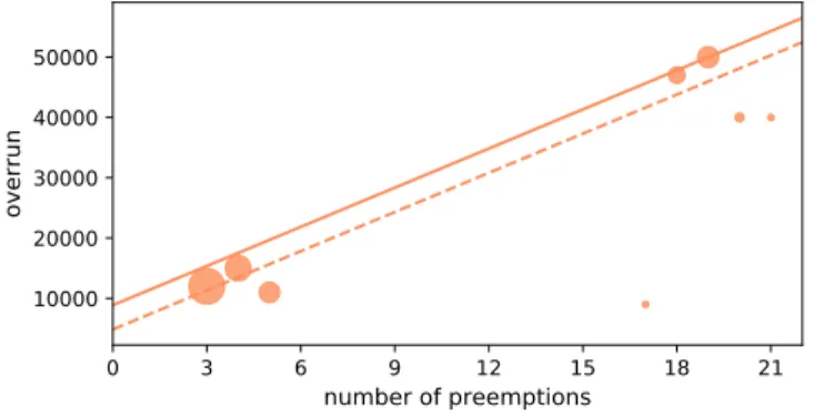
Figure 5 depicts a scatter plot of samples for a fixed e= 1

from an experiment similar to those presented in Section V; the size of the markers correlates to the weight of the sample. The figure also shows the regression function that results from the least squares method (dashed line), which is not yet an upper bound for the samples but basically settles the slopeP of the regression function. Second, we can calculate E from the samples such that the resulting regression function serves as an upper bound (solid line).

IV. RELATED WORK

The concept of self-awareness in computing systems was first proposed for autonomic computing in 2003 [24]. Today, there exists a large body of research in the field of self-awareness in computing systems [25], [26]. Self-aware com-puting systems employ architectural concepts that allow the system to observe (self-awareness) and adapt (self-expression) itself (cf. [14]). These concepts have been most recently surveyed and classified by Giese et al. [27], [28], who describe self-aware computing as a “paradigm shift from a reactive to a proactive operation that integrates the ability to learn, reason, and act at runtime [based on models]” [27].

Task graphs are a common vehicle for modelling application timing in order to perform response-time analyses. Precedence relations between tasks are reflected in task graphs of different

expressiveness [16]. Yet, although these models may have a notion of limited preemptability [17], they rarely incorporate the non-reentrant nature of single-threaded address spaces that leads to blocking. Modelling precedence and blocking relations in real-time applications to perform response-time analyses has been addressed by MAST [29], which bases on MARTE UML [30]. In MAST,scheduling serversmodel the schedulable entity whereas operations model activities that may lock/unlock a shared resource and that are mapped to scheduling servers.Transactionsare made of operations with their precedence relations, which are thus executed on differ-ent scheduling servers (i.e. priorities) so that bounding their latency requires specialised techniques [31]. Most recently, Schlatow and Ernst augmented the task-graph model with scheduling contexts and execution contexts in order to reflect the thread dualism.

W.r.t. modelling (real-time) workload, Wandeler et al. [19] have formulated workload curves that are semantically similar to the ET model [18]. The latter, in contrast, explicitly targets varying execution times and the extraction from traces. By transforming these curves into Workload Arrival Functions (WAFs), a Compositinal Performance Analysis [32] or Real-Time Calculus [33] can be used to check schedulability and calculate worst-case response times. In contrast to demand bound functions [34], WAFs do not include a notion of deadlines or schedulability. Neukirchner et al. [20] applied monitoring of WAFs by rejecting incoming events if their assumed WCET, in conjunction with the trace of previous executions, will violate the WAF. Violations trigger an excep-tion that can be handled at applicaexcep-tion level, which enable implementation of static mixed-criticality scheduling [3].

Another line of work that provides temporal isolation is sporadic server scheduling (and similar techniques). First mentioned by Sprunt et al. [15], it received attention as efficient and correct implementations are challenging [4], [5], [35]. Hence, approximate implementations exist that simplify these issues by assuming the same replenishment period Rt for all threads [36], [37]. QNX [37] manages replenishments by dividing the replenishment period into 1 ms slots that store the consumed budget. Accounting is performed on any OS tick or syscall. Lyons et al. [2] implemented sporadic server scheduling for the seL4 microkernel to achieve temporal isolation and to implement scheduling-context capabilities, which are temporal capabilities [38]. They use a tickless implementation based on the algorithm by Stanovich et al. [4]. The implementation can manage 8-10 replenishments at least whereas the actual replenishment threshold can be increased by user-level policies as well as the budget and replenishment period using their concept of scheduling-context capabilities. They introduce timeout exceptions as a mechanism to handle budget expirations at user level. Although being a quite so-phisticated solution, sporadic server scheduling approximates real-time workload as periodic tasks, which prevents WCRT analysis of using more exact task models.

Regarding overhead accounting, Stanovich et al. [5] take the opposite approach to accounting of preemption overheads

Table I

OVERHEAD MEASUREMENTS FROM MANUAL INSTRUMENTATION

name formula cycles µs

min. preemption overhead mini(tSi−tAi) 260 0.4

max. preemption overhead maxi(tSi−tAi) 3580 5.4

max. expiration overhead maxi(tSi−tKi−1) 8052 12.1 max. kernel lock overhead maxi(tKi−tKi−1) 23239 34.9

calculation overhead Eq. (1) with L=10 336 0.5

as they deduct an estimate of the preemption cost from the budget at run time, i.e.Q≤0 in Definition 1.

W.r.t. tracing, it is worth mentioning that many kernels provide built-in mechanisms for lightweight instrumentation and for extracting traces, such as the Ftrace2_{for Linux or the}

QNX System Analysis Toolkit [39]. Ftrace is, e.g., used by rt-muse[40] for extracting supply bound functions from different scheduling implementations in Linux.

V. EVALUATION

We implemented and tested our mechanisms from Sec-tion III on an ARM Cortex A9 dual-core SoC. Before pro-ceeding to our experimental evaluation, we first give a brief account of some noteworthy implementation details.

Internally, the kernel uses timer ticks to measure time so that a budget, which is provided in microseconds, must be con-verted into timer ticks. The SoC is running at 666.6666 MHz based on an oscillator clock of 33.33333 MHz. For time accounting (OS time), the kernel uses the Cortex-A9 CPU private timer with a clock divider of 100, which results in 3.333333 MHz or 200 CPU cycles per timer tick.

The kernel converts microseconds into timer ticks by integer multiplication with 3333 and division by 1000. Due to this in-teger calculation, in contrast to a multiplication with 3333.333, we have a systematic time drift of 0.0001, i.e. 100µs per second. We correct this by adding this fraction to the budget whenever the budget will be configured.

For reference, we measured the particular overheads men-tioned in Section II-C by manual instrumentation using the cycle counter from the Performance Monitoring Unit (PMU). Table I shows the results taken from several measurements with different workloads; one microsecond has 666.666 cycles. Note, that we measured the expiration overhead without the kernel lock, i.e. after the kernel lock was acquired. Con-ceptually, the only additional runtime overhead from our replenishment policy comes from calculating Eq. (1) on signal reception.

Memory overhead originates from storing aET+(n)curve per thread, the history of consumed budgets and the current budget, which constitutes L·8 +L·8 + 1Bytes as we use 64 Bit integers for each value. We used L = 10 in our implementation.

We configured our test setup for a maximum rate of 8000 trace events per second, which equates a preemption every

2_{http://elinux.org/Ftrace}

125µson average. As a trace event takes up 28 Bytes in the trace buffer, we require at most 224 KiBytes per second.

With the following evaluation we want to demonstrate the overhead monitoring can deal with different workloads and also a high rate of trace events. We also show thatET+_(n) curves can be extracted at run-time such that the budget configuration can be refined (after schedulability analysis). For these purposes, we defined three conceptually different workloads.

A) A single task chain with a ET+(n) curve of length nine. The chain shows synchronous and asynchronous precedence but there is no interference apart from self-interference.

B) Ten independently triggered components with a single-valued ET+_{(n), which impose a high CPU load. This} scenario focuses on interference.

C) Multiple task chains similar to experiment A. The chains perform RPCs to a single server component. This scenario combines the two previous experiments and introduces the blocking aspect.

For each workload, we evaluated the observed P and E values from our approximation method and compare these with the optimum that we calculated offline using an LP formulation and with the reference values from Table I.

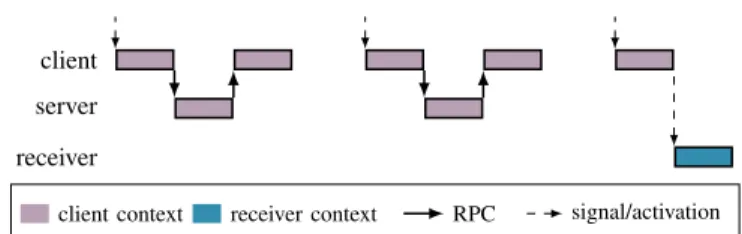
A. Single chain

The workload in this experiment consists of a client that is periodically activated and calls a server in two out of three activations as depicted in Figure 6. Every third activation, the client sends a signal to a receiver instead of calling the server. Due to scheduling-context donation, the server executes on the budget of the client.

client server receiver

client context receiver context RPC signal/activation

Figure 6. Gantt chart for the task chain used in experiment A. The client and server are implemented such that the required budget varies between 80 ms and 1500 ms and repeats every 10th activation. We configured the corresponding ET+(n)

such that the budget is exceeded by up to 200µs in approx. 50% of the times. We also chose a large activation period of 10 s, which is half the sample period of the monitor, in order to get a notion of how the overhead estimation develops with a growing sample size.

Figure 7 shows the resultingP andE for different sample sizes, i.e. the summed weights of all recorded weighted sam-plesΩˆp,e. As the sample size grows slowly in this experiment, it correlates with the iteration number of the monitor. Note, that there were up to 13 distinct weighted samples (i.e. com-binations of preemption number and expiration number). The

0 20 40 60 80 100 120

number of samples

overhead [ns]

Figure 7. Overhead monitoring results from experiment A.

approximate results (markers) from the modified least squares method are compared to the optimum results (solid lines) that we calculated offline. The figure also shows the measured preemption overhead (dashed line) from Table I. Note, that the maximumEbased on these measurements is 47 us (expiration overhead including kernel lock overhead) and exceeds the limits of the figure. Although this experiment is rather simple, it demonstrates the general applicability of ET+_{(n) shaping} and monitoring, and emphasises how the estimated overheads develop with a growing number of samples.

B. Independent tasks

This experiment comprises 10 independent tasks with peri-ods from 3 ms to 10 ms and execution times from 200µs to 900µs for the first eight tasks. In order to provoke preemp-tions, the two remaining tasks were assigned periods of 100 ms and 200 ms and execution times of 10 ms and 20 ms. The tasks have a rate-monotonic priority assignment (smallest period on highest priority) and impose a load of approx. 85% on the CPU core. However, due to the signalling implementation of the OS, activations are dropped in overload situations, i.e. if the receiver is not ready for receiving a signal. Each task is configured with ET+_{(n) of length one; most of the tasks} exceed their budget most of the times. However, as a task that used its budget cannot preempt other tasks (with budget) any more, we let the higher-priority tasks adhere to their budget in order to stimulate multiple preemptions. In contrast to the previous experiment, this workload produces many events such that every few seconds the traced execution times are completely overwritten. Furthermore, it is tailored for testing our monitoring approach w.r.t. whether it can deal with a high trace-event rate.

Figure 8 shows the resultingP andEfor this use case over time. Due to the high execution rate, the sample size saturates very quickly such that the x-axis shows the iteration number (i.e. the execution of the monitor) instead. Because of the single-valued ET+_{(n), our monitoring also shifts a window} of length one over the traces. Thus, the maximum observed expiration number is always one, such that the samples only

0 20 40 60 80 100

number of monitor iterations

0 10000 20000 30000 40000 50000

overhead [ns]

Figure 8. Overhead monitoring results from experiment B.

differed in the number of preemptions of which there were 21 distinct numbers on average (standard deviation 1.5). As the samples do not indicate a correlation between the preemption number and the overrun, the resulting P is zero most of the times (negative values are forbidden in the model). This holds for both, our approximation method as well as the LP-based optimisation. In consequence, most of the overhead is attributed to E, which still remains below the measured overheads from Table I.

C. Multiple chains

This experiment basically combines experiments A and B. We split the chain of experiment A into three chains of similar structure and execution times between 5 ms and 80 ms. The resulting workload comprises three clients, three receivers and a single server that is called by all clients. The clients are periodically triggered every 100 ms and have a ET+_{(n) of} length three. We set the execution times such that the system is transiently overloaded to stimulate preemptions and blocking at the server. The longest execution time of the server is 11 ms, which occurs if the lowest-priority client calls the server. In theory, we should be able to observe that the high-priority client requires up to 11 ms more budget if it acts as a helper for the lowest-priority client.

1 2 3 4

n

ET

(n

) [ms]

n

n

n

Figure 9. Configured and extractedET+_{(n)curves of the highest-priority} client in experiment C.

In order to demonstrate the self-aware adaptation of budgets, we started with an ET+_{(n) that neglects blocking effects}

at the server, which underestimates the required budget. By applying budget monitoring to extract the actual ET+_(n), we can iteratively adapt the configured budget (if schedu-lability analysis approves) and react to the observed model deviation. Figure 9 illustrates these adaptations on basis of the observed ET+_{(n) curve of the highest-priority client.} After three adaptations, we found the curve that bounds the required execution time of the highest-priority client. It requires multiple iterations because once the highest-priority budget expired, the medium-priority client also acts as a helper. The result is consistent with our expectation as it can be calculated by adding the longest blocking time (11 ms) to the second longest execution of the highest-priority client. Due to the synchronised hyper-periodic behaviour of the clients, the blocking cannot coincide for the longest execution. Note, that – if the application timing model is known – we could also start with an overestimatedET+_{(n)by adding the longest} blocking times and extracting the sameET+_{(n)as above after} the first adaptation.

0 20 40 60 80 100

number of monitor iterations

0 5000 10000 15000 20000 25000 30000 35000

overhead [ns]

Figure 10. Overhead monitoring results from experiment C. Figure 10 depicts the resulting overheads for this experiment for the first 100 monitor iterations after the last budget adapta-tion. As in the previous experiments, the estimated overheads are below our measurements from Table I. There was an average of 21 distinct samples (standard deviation 1.6). The regression still shows significant variations of the estimated expiration overhead. However, as even the results from our offline LP optimisation shows variations, it becomes evident that averaging or maximisation is required over a longer time frame. For illustration, we added the moving average ofE to Figure 10 (dotted line). These variations can be explained by the kernel lock overhead that occurs rarely and varies in length. The estimation is therefore sensitive to whether an occurrence (sample) with a large kernel lock time resides in the trace or not. Such an occurrence will eventually be replaced by newer samples.

VI. CONCLUSION

Latency guarantees in real-time systems are based on mod-els on which formal analyses are performed. As modmod-els always

abstract from a reality, there exists a large body of research for refining and improving these models in order to capture reality more accurately and to improve latency bounds. E.g. analyses should consider implementation overheads and corner cases that originate from particularities in real implementations. However, it is commonly known that there is no guarantee that a model is coherent with the implementation even though it is an important interface for applying formal methods. A practical implication of this incoherence is that it highly impedes the application and acceptance of (i.e. the trust in) formal methods. We consider self-aware computing as a practical mitigation to model-implementation incoherence. In this paper, we suggested applying this concept to CPU scheduling. For this purpose, we derived a kernel timing model from an existing budget scheduling implementation. In order to adapt the scheduling to better suit real-time workloads, we implemented a novel event-based replenishment policy based onET+_{(n)curves. In contrast to existing policies, our} approach is conceptually lightweight as it eliminates replenish-ment fragreplenish-mentation. As as side effect, this reduces the number of context switches as a correct budget configuration ensures that a job can complete without running out of budget. On top of this, we implemented a budget monitoring and overhead monitoring mechanism based on software-based tracing of the scheduler. Overhead monitoring checks and guarantees the adherence of the implementation to our kernel timing model, which is essential for limiting interference. Budget monitoring, on the other hand, enables the extraction ofET+(n)functions. As we showed in our last experiment, the latter can be ap-plied to characterise applications with an unknown or uncertain timing model. In order to correctly execute those applications (but still limit their interference on other applications), the ET+_{(n) must be sufficiently large but also tight. For this} purpose, we envision the following use case that is enabled by our approach: A mixed-critical real-time system can receive an application update with an unknown timing model. This can be executed (e.g. using sandboxing techniques) with an overes-timated budget on a low priority such that other applications are not interfered. This serves as a first basis for extracting theET+_{(n)using budget monitoring. As this budget is more} tight, we can move the application to a higher priority to achieve the required latency. Over time, theET+(n)curves in the system can be further refined to free up more processing resources for future changes/updates.

Our evaluation showed that the tracing of scheduling be-haviour and monitoring of scheduling overheads is feasible even for high trace-event rate and complex workload. Nev-ertheless, the regression method requires some improvement (e.g. averaging) to get more stable results that can be used for learning from observed behaviour in the long term. We are confident that our models and mechanisms are applicable to other (similar) kernels as well. Since our monitoring (on kernel timing model) includes notions of budgets and overheads only, the concept of self-awareness should also be applied to the application timing model, in order to gain knowledge about from what component a misbehaviour originates.

ACKNOWLEDGEMENT

This work was funded as part of the DFG Research Unit

Controlling Concurrent Change, funding number FOR 1800.

REFERENCES

[1] R. Ernst and M. D. Natale, “Mixed Criticality Systems - A History of Misconceptions?”IEEE Design & Test, vol. 33, no. 5, Oct. 2016. [2] A. Lyons, K. Mcleod, H. Almatary, and G. Heiser, “Scheduling-context

capabilities: A principled, light-weight OS mechanism for managing time,” inEuroSys Conference. Porto, Portugal: ACM, Apr. 2018. [3] S. K. Baruah and A. Burns, “Response-time analysis for mixed criticality

systems,” inIn Proceedings of the IEEE Real-Time Systems Symposium, 2011.

[4] M. Stanovich, T. Baker, A.-I. Wang, and M. Harbour, “Defects of the posix sporadic server and how to correct them,” in Real-Time and

Embedded Technology and Applications Symposium (RTAS), Stockholm,

Sweden, 04 2010, pp. 35–45.

[5] M. J. Stanovich, T. P. Baker, and A. i Andy Wang, “Experience with Sporadic Server Scheduling in Linux: Theory vs. Practice,” inReal-Time

Linux Workshop, 2011.

[6] N. Feske, “Genode OS Framework Foundations 18.05,” Tech. Rep., May 2018. [Online]. Available: http://genode.org/documentation/ genode-foundations-18-05.pdf

[7] Genode OS Framework release notes 16.11, 17.08, 18.02 and 18.08. [Online]. Available: https://genode.org/documentation/release-notes/ index

[8] M. M¨ostl and R. Ernst, “Cross-layer dependency analysis with timing dependence graphs,” in Proceedings of the 55th Design Automation

Conference (DAC), 2018.

[9] J. Schlatow and R. Ernst, “Response-time analysis for task chains in communicating threads,” in22nd IEEE Real-Time Embedded Technology

and Applications Symposium (RTAS 2016), Vienna, Austria, Apr. 2016.

[10] U. Steinberg, A. B¨ottcher, and B. Kauer, “Timeslice Donation in Component-Based Systems,” inIntern. Workshop on Operating Systems

Platforms for Embedded Real-Time Applications (OSPERT), Brussels,

Belgium, 2010.

[11] G. Parmer, “The Case for Thread Migration: Predictable IPC in a Customizable and Reliable OS,” in Intern. Workshop on Operating

Systems Platforms for Embedded Real-Time Applications (OSPERT),

Brussels, Belgium, 2010.

[12] J. Schlatow and R. Ernst, “Response-time analysis for task chains with complex precedence and blocking relations,”International Conference on Embedded Software (EMSOFT), ACM Transactions on Embedded

Computing Systems ESWEEK Special Issue, vol. 16, no. 5s, pp. 172:1–

172:19, sep 2017.

[13] A. Lackorzy´nski, A. Warg, M. V¨olp, and H. H¨artig, “Flattening hier-archical scheduling,” inProceedings of the Tenth ACM International

Conference on Embedded Software, ser. EMSOFT ’12. New York, NY,

USA: ACM, 2012, pp. 93–102.

[14] P. R. Lewis, A. Chandra, S. Parsons, E. Robinson, K. Glette, R. Bahsoon, J. Torresen, and X. Yao, “A survey of self-awareness and its application in computing systems,” in Proceedings of the 2011 Fifth IEEE

Con-ference on Self-Adaptive and Self-Organizing Systems Workshops, ser.

SASOW ’11. Washington, DC, USA: IEEE Computer Society, 2011, pp. 102–107.

[15] B. Sprunt, L. Sha, and J. Lehoczky, “Aperiodic task scheduling for hard-real-time systems,”Real-Time Systems, vol. 1, no. 1, pp. 27–60, Jun 1989.

[16] M. Stigge, “Real-time workload models: Expressiveness vs. analysis efficiency,” Ph.D. dissertation, Uppsala University, 2014.

[17] P. Fradet, X. Guo, J.-F. Monin, and S. Quinton, “A Generalized Digraph Model for Expressing Dependencies,” inRTNS ’18 - 26th International

Conference on Real-Time Networks and Systems, Chasseneuil-du-Poitou,

France, Oct. 2018, pp. 1–11.

[18] S. Quinton, M. Hanke, and R. Ernst, “Formal analysis of sporadic overload in real-time systems,” inDesign, Automation & Test in Europe

Conference & Exhibition(DATE), vol. 00, 03 2012, pp. 515–520.

[19] E. Wandeler, A. Maxiaguine, and L. Thiele, “Quantitative characteriza-tion of event streams in analysis of hard real-time applicacharacteriza-tions,”

Real-Time Systems, vol. 29, no. 2, pp. 205–225, Mar 2005.

[20] M. Neukirchner, P. Axer, T. Michaels, and R. Ernst, “Monitoring of workload arrival functions for mixed-criticality systems,” in Proc. of

Real-Time Systems Symposium (RTSS), dec 2013.

[21] M. Neukirchner, T. Michaels, P. Axer, S. Quinton, and R. Ernst, “Monitoring arbitrary activation patterns in real-time systems,” inProc.

of IEEE Real-Time Systems Symposium (RTSS), dec 2012.

[22] M. Beckert, M. Neukirchner, S. M. Petters, and R. Ernst, “Sufficient temporal independence and improved interrupt latencies in a real-time hypervisor,” inProc. of Design Automation Conference (DAC), Jun 2014. [23] M. Stein. (2017, Feb.) A kernel in a library: Genode’s custom kernel approach. FOSDEM. Brussels, Belgium. [Online]. Available: https: //archive.fosdem.org/2017/schedule/event/microkernel kernel library/ [24] J. O. Kephart and D. M. Chess, “The vision of autonomic computing,”

Computer, vol. 36, no. 1, Jan. 2003.

[25] Peter R. Lewis, Marco Platzner, Bernhard Rinner, Jim Tørresen, and Xin Yao,Self-aware Computing Systems - An Engineering Approach. Springer International Publishing, 2016.

[26] S. Kounev, J. O. Kephart, A. Milenkoski, and X. Zhu, Eds.,Self-Aware

Computing Systems. Cham: Springer International Publishing, 2017.

[27] H. Giese, T. Vogel, A. Diaconescu, S. G¨otz, N. Bencomo, K. Geihs, S. Kounev, and K. L. Bellman,State of the Art in Architectures for

Self-aware Computing Systems. Cham: Springer International Publishing,

2017.

[28] H. Giese, T. Vogel, A. Diaconescu, S. G¨otz, and S. Kounev,

Architec-tural Concepts for Self-aware Computing Systems. Cham: Springer

International Publishing, 2017, pp. 109–147.

[29] (2015) MAST 1.5.0: Description of the mast model. [Online]. Available: http://mast.unican.es/mast description.pdf

[30] (2009-2011) MARTE UML: modeling and analysis of real-time embedded systems. [Online]. Available: http://www.omg.org/spec/ MARTE/

[31] M. G. Harbour, M. H. Klein, and J. P. Lehoczky, “Fixed priority scheduling periodic tasks with varying execution priority,” in12th

Real-Time Systems Symposium, Dec 1991, pp. 116–128.

[32] R. Henia, A. Hamann, M. Jersak, R. Racu, K. Richter, and R. Ernst, “System Level Performance Analysis - the SymTA/S Approach,” in

IEEE Proceedings Computers and Digital Techniques, 2005.

[33] L. Thiele, S. Chakraborty, and M. Naedele, “Real-time calculus for scheduling hard real-time systems,” inin ISCAS, 2000, pp. 101–104. [34] I. Shin and I. Lee, “Compositional real-time scheduling framework,”

in Proceedings of the 25th IEEE International Real-Time Systems

Symposium, ser. RTSS ’04. Washington, DC, USA: IEEE Computer

Society, 2004, pp. 57–67.

[35] D. Faggioli, M. Bertogna, and F. Checconi, “Sporadic server revisited,”

in In SAC ’10: Proceedings of 25th ACM Symposium On Applied

Computing. ACM, 01 2010, pp. 340–345.

[36] M. Beckert, K. B. Gemlau, and R. Ernst, “Exploiting sporadic servers to provide budget scheduling for arinc653 based real-time virtualization environments,” in Proc. of Design Automation and Test in Europe

(DATE), Lausanne, Switzerland, March 2017.

[37] (2006, Jun.) QNX Adaptive Partitioning: the How it Works FAQ. [Online]. Available: https://community.qnx.com/sf/wiki/do/viewPage/ projects.core os/wiki/APS How it Works FAQ

[38] P. K. Gadepalli, R. Gifford, L. Baier, M. Kelly, and G. Parmer, “Temporal capabilities: Access control for time,” in 2017 IEEE

Real-Time Systems Symposium (RTSS), Dec 2017, pp. 56–67.

[39] (2018) QNX System Analysis Toolkit User’s Guide. [Online]. Available: http://www.qnx.com/developers/docs/7.0.0/#com.qnx.doc.sat/ topic/about.html

[40] M. Maggio, J. Lelli, and E. Bini, “rt-muse: measuring real-time charac-teristics of execution platforms,”Real-Time Systems, vol. 53, no. 6, pp. 857–885, Nov 2017.