Back to Keynes?

B

ACK TO

K

EYNES

?

F

REDERICK VAN DER

P

LOEG

CES

IFO

W

ORKING

P

APER

N

O

.

1424

C

5:

F

P

,

M

G

M

2005

An electronic version of the paper may be downloaded • from the SSRN website: www.SSRN.com

B

ACK TO

K

EYNES

?

Abstract

After a brief review of classical, Keynesian, New Classical and New Keynesian theories of

macroeconomic policy, we assess whether New Keynesian Economics captures the

quintessential features stressed by J.M. Keynes. Particular attention is paid to Keynesian

features omitted in New Keynesian workhorses such as the micro-founded Keynesian

multiplier and the New Keynesian Phillips curve. These theories capture wage and price

sluggishness and aggregate demand externalities by departing from a competitive framework

and give a key role to expectations. The main deficiencies, however, are the inability to

predict a pro-cyclical real wage in the face of demand shocks, the absence of inventories,

credit constraints and bankruptcies in explaining the business cycle, and no effect of the

nominal as well as the real interest rate on aggregate demand. Furthermore, they fail to allow

for quantity rationing and to model unemployment as a catastrophic event. The

macroeconomics based on the New Keynesian Phillips curve has quite a way to go before the

quintessential Keynesian features are captured.

JEL Code: E12, E32, E63.

Keywords: Keynesian economics, New Keynesian Phillips curve, monopolistic competition,

nominal wage rigidity, welfare, pro-cyclical real wage, inventories, liquidity, bankruptcy,

unemployment, monetary policy.

Frederick van der Ploeg

Robert Schuman Centre

European University Institute

Badia Fiesolana

Via dei Roccettini 9

50016 San Domenico di Fiesole (FI)

Italy

[email protected]

I have benefited from stimulating comments from Roel Beetsma, Bas Jacobs, Bill Martin,

Bob Rowthorn and the participants in the CESifo Venice Workshop on ‘Aggregate demand

management policies: Back to Keynes’, 19-20 July 2004. Given the huge literature on the

various schools of macroeconomic thought, I present an eclectic view of developments in

Keynesian macroeconomics and conclude with some lessons and challenges for the

development of New Keynesian economics.

1. Introduction

The macroeconomic debates on the effectiveness of fiscal and monetary policy have raged for many decades on both sides of the Atlantic. An influential and readable reinterpretation of the economics of J.M. Keynes is Leijonhufvud (1968). Up to the seventies many economists and policy makers believed in a neo-Keynesian trade-off between inflation and unemployment, so that an expansionary fiscal or monetary policy would at least boost employment and lower unemployment for some time. The accelerator hypothesis popular in the seventies insisted that extra jobs could only be achieved at the expense of ever-increasing inflation. The critique of econometric policy evaluation put forward by Lucas (1976), the insistence on people not being fooled all the time, and the subsequent outburst of New Classical Economics led by Lucas (1972, 1973) and Sargent and Wallace (1975) killed the popularity of Keynesian economics. By the end of the seventies policy makers and economists became sceptical about the possibility of expansionary demand management lowering unemployment. The rationing theories of aggregate demand put forward by Barro and Grossman (1971) and Malinvaud (1977) are ingenious, but came at the wrong time and did not explain why wages and prices are rigid. They quickly found their ways to the bottom of the filing cabinets. With the supply-side policies advocated by Mrs. Thatcher and Mr. Reagan economists changed tack completely. During the eighties and the nineties the fresh-water economists have made inroads into the profession. Many of the brightest graduates of that period followed in the footsteps of Robert E. Lucas, Edward Prescott, Thomas Sargent and others and rejected the Keynesian and neo-Keynesian theories of aggregate demand with sluggish price and wage formation. Instead, they insisted on modelling dynamic, competitive general equilibrium models with rigorous micro foundations, rational expectations and prices and wages adjusting instantaneously to clear all goods and labour markets. In these real business cycle models fluctuations arise from technology shocks rather than from changes in economic policy. In this sense, this generation of economists is the descendant of classical economists like Adam Smith, David Hume, David Ricardo, John Stuart Mill, Knut Wicksell, Irving Fisher and John Maynard Keynes of The Treatise of Money of 1930 who also insisted that output is primarily determined by productive capacity.

However, in the eighties Hart (1982), Blanchard and Kiyotaki (1987), Cooper and John (1988), Mankiw (1990) and others collected in Mankiw and Romer (1991) explained that aggregate demand externalities in economies with monopolistic competition can produce Keynesian multipliers. Mankiw (1985), Akerlof and Yellen (1985) and Parkin (1986) showed that with small menu costs prices can be rigid and monetary policy has real effects on the economy. More recently, Michael Woodford, Jordi Galí and others have continued the New Keynesian counter-attack on the real business cycle orthodoxy. Their objective is to develop dynamic, non-competitive general equilibrium models with rigorous micro foundations, but

where it is costly to adjust prices instantaneously. They obtain a micro-founded, forward-looking New Keynesian Phillips curve with a short-run trade-off between inflation and unemployment. The main advantage is that a second-order approximation to a proper micro-founded welfare loss function could be obtained. This led to the advice that central bankers should not target the actual output gap, but should target the economy as close as possible to the level of output that would have prevailed under flexible wages and prices. This advice only works if the right level corrective taxes and subsidies ensure that the flexible price equilibrium is first best and, in particular, correct for the distortions arising from non-competitive behaviour. Monetary policy can then concentrate on correcting the temporary distortions of relative prices. However, the New Keynesian Phillips curve has some problems explaining that inflation displays inertia and monetary disinflations are contractionary.

This paper spells out in a little more detail these developments in macroeconomic theory during the last four decades. Table 1 summarises the main persona and ideas of the various schools of macroeconomic thought and shows in which part of the paper they are discussed. Hopefully, this puts recent advances in macroeconomic theory in a better perspective. An attempt is made to assess whether New Keynesian economics captures the quintessential features stressed by J.M. Keynes. Particular attention is paid to New Keynesian workhorses such as the micro-founded Keynesian multiplier and the New Keynesian Phillips curve. These theories capture wage and price sluggishness and aggregate demand externalities in a framework of monopolistic competition and give a key role to expectations. The main deficiencies, however, are the inability to predict a pro-cyclical real wage in the face of demand shocks, the absence of inventories, credit constraints and bankruptcies in explaining the business cycle, and the absence of an effect of the nominal as well as the real interest rate on aggregate demand. Furthermore, they fail to distinguish between effective and notional demands and supplies, to model unemployment as a catastrophic event and to allow for psychological features such as downward rigidity of wages and not taking account of the full effects of changes in inflation at low rates of inflation.

Section 2 summarises the classical view of macroeconomics and the crucial role played by the labour market and distortions such as the tax wedge. It explains that government spending is fully crowded out by falls in investment, consumption and net exports, and more than fully crowded if financed by taxes on labour. The classical multiplier is thus likely to be negative. It also argues that money is neutral in the classical view. Section 3, in contrast, puts forward the Keynesian view and the crucial role of aggregate demand management. It explains that the Keynesian multiplier is positive and weakened by leakages from saving, taxation and imports, financial crowding out, and automatic stabilisers. Section 3 also discusses the Keynesian multipliers for a small open economy and the assignment of monetary or fiscal policy to aggregate demand in a stochastic economy. Furthermore, it

reviews the general equilibrium features of the macroeconomics of quantity rationing, the micro underpinnings that have been given for the Keynesian multiplier and the rigidity of prices, and the role of credit rationing and financial intermediaries in determining aggregate demand. Section 4 highlights various attempts at a neo-Keynesian synthesis between classical and Keynesian views. The Phillips curve, the accelerator hypothesis, the ongoing battle of the mark-ups and the pro-cyclical real wage, overlapping wage contracts, near-rational wage and price setting, and keeping up with the Joneses are discussed. Section 5 discusses the Lucas critique and the New Classical economics and real business cycle theory. Section 6 critically examines the most recent theories of the New Keynesian Phillips curve. Section 7 discusses their deficiencies from a Keynesian point of view, and offers suggestions for future research.

2. The classical view of macroeconomics

The classical view on macroeconomic policy presumes that all markets clear immediately. All unemployment is voluntary and corresponds to freely chosen leisure or 'holidays'. In addition, unemployment may reflect voluntary engagement in non-market transactions, such as the provision of household and caring services. These exchanges of real resources are not captured in the employment statistics. Nevertheless, there is reason for concern if many people choose too much leisure or participate too much in non-market activities. The fall in labour supply erodes the tax and premium base and threatens the welfare state. The New Right advocates cutting the tax burden and the size of government in order to improve labour market participation and private sector incentives.

2.1. Key role for productive capacity and the labour market

The classical view gives the labour market the limelight in determining aggregate employment and national income. Labour demand declines with the producer wage, wP≡ W(1+t1)/P where

W, P and t1 are the nominal wage, the producer price and the rate of employers' taxes and

contributions, respectively. A higher product wage induces firms to shed labour until the marginal product of labour has risen to the new producer wage. Labour supply depends on the consumer wage, wC≡ W(1-t2)/P(1+t3) where t2 and t3 denote the employees' rate of taxes and

premiums and indirect tax rate, respectively. A higher consumer wage makes leisure more expensive and thus induces households to work more hours (substitution effect). It also raises income, so households work fewer hours (income effect). Labour supply thus bends backwards for high levels of the consumer wage. Empirical studies suggest that labour supply of males is fairly inelastic, i.e., the income effect wipes out most of the substitution effect, but labour supply of females is more elastic. Labour supply at the extensive margin is more elastic, that is

the decision whether to participate or not in the labour market is more sensitive to changes in the wage than the decision how many hours to work.

The difference between what a worker costs a company and what a worker can spend is the tax wedge, t ≡ (wP-wC)/wP≈ t1+t2+t3. The tax wedge is the sum of the indirect tax rate, the

employers' tax and premium rate and the employees' tax and premium rate. A higher tax wedge reduces labour supply, pushes up the product wage, lowers the consumer wage, and depresses employment and economic activity. With perfect competition it does not matter whether employers or households pay the taxes on labour. Part of the burden of the higher employees' tax rate is passed on to firms, especially if labour demand is relatively inelastic and labour supply is elastic. Similarly, firms shift some of the incidence of the employers’ tax to workers by reducing the wage, especially if labour supply is inelastic and labour demand is elastic.

In the seventies many countries tried to cure unemployment by cutting labour supply through a general reduction in working hours, early retirement, etc., because it was clear that a Keynesian response to stagflation would be counter-productive. This is the fallacy of the fixed number of jobs: if the employed work less hours, some unemployed can have a job as well. The classical view rightly argues that this pushes up the wage and reduces the demand for labour. Cutting labour supply grinds the economy to a lower level of economic activity, making the lucky ones with a job better off and dumping in the longer run even more people on the dole.

2.2. Crowding out and effects on saving, investment, budget deficit and trade balance

Demand-side policies do not affect employment or national income, so the classical multiplier for a bond-financed increase in public spending is zero. The classical tax-financed multiplier for public spending is negative, since the associated rise in the tax wedge curbs labour supply and thus decreases national income. A rise in public spending is thus (more than) fully crowded out by falls in the other components of aggregate demand. The mechanism is a rise in the interest rate caused by the government selling bonds to the public. Since domestic bonds become relatively more attractive than foreign bonds, capital flows in from abroad. The associated rise in the demand for domestic currency induces an appreciation of the currency. The higher interest rate generally boosts private saving and reduces private consumption, and depresses aggregate investment. The appreciation of the currency cuts net exports. The higher budget deficit thus leads to a trade deficit as well. With bond finance the rise in public spending is exactly offset by the fall in private consumption, investment and net exports. With tax finance it is more than fully offset, so that employment and output fall.

This type of crowding out presumes that government debt and real capital assets are close substitutes in private asset portfolios. In general, a higher supply of bonds induces excess supply in the bond market and excess demand for funds in the markets for money and real capital assets. To restore equilibrium in financial markets, the price of bonds falls and the return

on bonds rises while the return on real capital falls. This reduces new investment. If bonds are closer substitutes for money than for real capital assets, the wealth effect raises demand for real capital assets and reduces the required return on new investment, thereby inducing crowding in of private investment.

The higher interest rate reduces money demand which raises the price level for a given nominal money supply. Hence, a bond-financed expansion of aggregate demand does not boost employment or national income but merely changes the composition of aggregate demand through a higher interest rate and price level and an appreciation of the currency.2 _{Money is thus}

neutral. An expansion of the money supply, achieved by buying bonds on the open market, merely leads to a proportional increase in prices and leaves employment, national income and the interest rate unaffected. Inflation is thus purely a monetary phenomenon and there is no role for demand-side policies. There may be a role for more public spending on material and immaterial infrastructure. If labour and capital are cooperative production factors, this boosts the demand for labour and raise both employment and the wage.

3. The Keynesian view: demand-side policies

In contrast, the Keynesian view argues that aggregate demand for goods, rather than the cost of labour, determines aggregate employment. This view is more pessimistic about the market clearing mechanism: prices and nominal wages are rigid in the short run. The economy has idle capacity and unemployed workers. Fiscal expansion may help to combat unemployment.

3.1. The textbook Keynesian multiplier: closed economy

The Keynesian multiplier for a rise in public spending was, in fact, for the case of a given interest rate derived by Kahn (1931) before the publication of Keynes (1936), namely the inverse of the marginal propensity to save. In general, the simultaneous determination of national income and the interest rate occurs in the IS-LM model popularised by Hicks (1937). Aggregate demand consists of private and public consumption, private and public investment, and net exports. It rises with national income and declines with the interest rate (and the value of the currency) and determines national income, giving rise to the familiar downward-sloping IS-curve. Money demand also rises with national income and falls with the interest rate, and must equal the real supply of money, leading to the upward-sloping LM-curve. Bond-financed fiscal expansion shifts out the IS-curve, which yields the familiar Keynesian bond-financed multiplier for a rise in public spending:

1/(1-MPC+MPM+CRO) =

2 _{With fixed exchange rates the central bank intervenes by selling home currency, thus boosting money}

1 + (MPC-MPM-CRO) + (MPC-MPM-CRO)2 + (MPC-MPM-CRO)3 + ... , where MPC is the marginal propensity to consume, MPM the marginal propensity to import and CRO financial crowding out. The marginal propensity to consume is MPC=c(1-t2) where c is

the marginal propensity to consume out of disposable income. The marginal propensity to save out of gross income is (1-c)(1-t2). Higher public spending, even of the hole-in-the ground

variety, sets in motion a multiplier process. To illustrate, set t2=0.25 and c=0.8 so that MPC=0.6

and the marginal propensity to save out of gross income is 0.15. If the government then spends hundred million euros on construction workers and we ignore imports and financial crowding out, workers save 15 million euros, pay 25 million euros in taxes and spend 60 million euros on consumption goods out of this extra income. The recipients of this additional expenditure save 9 million euros, pay 15 million euros in taxes, and spend another 36 million euros. This eventually expands private consumption by 150 million euros. Together with the initial increase in public spending, this yields a total expansion of national income of 100+60+36+..=250 million euros, corresponding to a multiplier of 2.5. Not all the expansion in income is consumed. Part of it leaks away via higher saving, 37.5 million euros, and higher taxes, 62.5 million euros. Bigger leakages from saving and taxes yield a smaller multiplier. If some of the additional expenditures are spent on foreign goods, e.g., MPM=0.4, the multiplier is reduced to 1.25. If aggregate demand is insensitive to the interest rate (a vertical IS-curve) and/or the economy is in a liquidity trap (a horizontal LM-curve), there is no financial crowding out (CRO=0). In general, however, the sale of government bonds needed to finance higher public spending pushes up the interest rate and lowers private consumption, investment and (through appreciation of the currency) net exports, thereby reducing the multiplier (as CRO>0). Financial crowding out is more significant (CRO large) if aggregate demand is more sensitive to the interest rate and the semi-elasticity of money demand with respect to the interest rate is small. If the rise in public spending is financed by higher taxes, we obtain the balanced-budget multiplier (1-MPC)/(1-MPC+MPM+CRO)≤1. This multiplier is smaller than under bond finance, because higher taxes reduce disposable income and depress private consumption and aggregate demand. With no imports and no financial crowding out, the balanced-budget multiplier is exactly one (Haavelmo, 1945).

If public spending is a close substitute for private spending, higher public spending reduces private spending and further dampens the Keynesian multiplier. Automatic stabilisers operate contra-cyclically, especially if benefits are substantial and the tax system is progressive. They reduce the Keynesian multiplier and make demand management less effective. In summary, the Keynesian multiplier is substantially reduced by leakages from saving, taxes and imports, financial crowding out, direct crowding out and tax finance and automatic stabilisers. In that case, exogenous shocks to aggregate demand (e.g. arising from changes in world trade) do not affect the economy much either.

Most of the well-known Keynesian macroeconometric models explain cycles due to various lags in the components of aggregate demand. In particular, the accelerator theory of investment allows current and past changes in output to affect the demand for investment goods. Much attention is always given to the dynamics of inventory accumulation (e.g., Blinder, 1981; Blinder and Fischer, 1981). These lags induce rich dynamic responses.

3.2. The textbook Keynesian multiplier: small open economy

The global capital market drives returns on financial securities close to each other. This affects the effectiveness of macroeconomic policy. With a floating exchange rate and perfect international capital mobility fiscal policy cannot be used to influence aggregate demand. A rise in public spending or a tax cut pushes up the interest rate and leads to incipient capital inflows. This induces appreciation of the currency and a switch in demand away from domestic goods towards foreign goods. The rise in public demand is exactly offset by a fall in net exports rendering unilateral fiscal expansion ineffective. Such economies are also well insulated from foreign shocks to aggregate demand. Monetary expansion, in contrast, is extremely powerful. The downward pressure on the domestic interest rate induces incipient capital outflows. The associated depreciation of the exchange rate boosts net exports and thus aggregate demand even further. With floating exchange rates a country is able to cushion the impact of an adverse external shock by allowing the exchange rate to depreciate. But this is not costless; it raises import prices and harms price stability. Monetary authorities may respond by tightening monetary policy and raising interest rates to prevent the exchange rate from falling. Economies are then only partially insulated from foreign shocks.

With fixed exchange rates monetary expansion, again achieved by purchasing bonds on the open market, causes incipient capital outflows. The central bank defends the currency by selling foreign reserves and purchasing own currency. The associated drop in money supply renders the initial monetary expansion completely ineffective; at the end of the day the central bank has merely changed foreign for domestic bonds. With a fixed exchange rate the domestic interest rate is tied to the foreign interest rate and cannot be used to combat unemployment. Fiscal expansions, in contrast, induce purchases of foreign reserves to prevent the currency from appreciating. The corresponding expansion of the money supply ensures that fiscal expansions are relatively powerful under pegged exchange rates.

3.3. Uncertainty and the appropriate Keynesian policy mix

Whether one should use the interest rate or the money supply to control aggregate demand in a Keynesian setting depends on where the shocks in the economy originate from. If shocks in goods demand are much more (less) volatile than shocks to money demand, the money supply (interest rate) is the appropriate instrument for managing aggregate demand (Poole, 1970). In

the open economy a regime of pegged exchange rates is ideal if shocks come mainly from money demand while a nominal income target is best if shocks occur primarily in goods demand (Bean, 1984). Other important rule of thumb are to make more use of instruments whose multipliers are known more precisely and to use a mix of policy instruments greater than the number of targets of economic policy (Brainard, 1967). Robust macroeconomic policies are supply-friendly fiscal expansions. A tax cut stimulates economic activity, irrespective of whether one is a Keynesian or a classical. In the former case, tax cuts raise disposable income and stimulate aggregate demand. In the latter case, tax cuts reduce the wedge between the producer and the consumer wage, and improve incentives for labour market participation and economic activity. Other robust policies are public investment or education with a market return. These boost the economy in Keynesian and classical worlds. Raising public consumption or public employment is not a robust fiscal policy. From the classical point of view, the rise in public spending is crowded out by falls in private spending. Most Keynesians recognise that the expansion of demand may come too late, due to a variety of recognition, decision and implementation lags, and be counter-productive. Supply-friendly policies such as tax cuts, public investment and education programmes may also be pro-cyclical due to recognition, decision and implementation lags. Fine-tuning is thus in practice difficult.

3.4. Macroeconomics of quantity rationing with micro foundations

During the seventies the Keynesians were under attack for being ad hoc and lacking serious microeconomic foundations. The first attempts to provide a micro underpinning for Keynesian economics were made by Barro and Grossman (1971) and Malinvaud (1977) and had two main features. First, given that the price system does not work, quantity signals take over from price signals as a coordination device. Second, general equilibrium interactions between labour, product and financial markets are important. Rationing in one market has spill-over effects in other markets and effective rather than notional demands and supplies matter. The Keynesian regime is characterised by generalised excess supply of labour and goods. Since households are involuntarily unemployed and cannot sell all the labour they want, their demand for goods is determined by their effective (constrained) labour supply. Firms cannot sell all the goods they want, so their demand for labour is constrained by the aggregate demand for goods. A Keynesian multiplier results, since boosting aggregate demand by cutting taxes or raising government spending raises employment and output. In contrast, the classical regime is characterised by excess supply of labour and excess demand for goods. Demand for labour is thus determined by the cost of labour alone and not constrained by lack of demand for goods. Since households can buy what they want but cannot sell all their labour, their supply of labour follows from labour demand and this determines how much they consume. The classical regime has a recursive solution: the cost of labour determines labour demand, which equals effective

supply of labour and gives aggregate output. The classical multiplier for government spending is thus negative. There is also a regime of repressed inflation characterised by generalised excess demand for goods and labour. In that case, the multiplier for government spending is negative as this worsens the queues of households in the shops. Households then even have less incentive to supply labour, since they cannot buy anything with their hard-earned cash.

In the classical regime the real wage must fall to fight unemployment. In contrast, the real wage should rise in the regime of Keynesian unemployment in order to boost aggregate demand for goods. This loosens the quantity constraint of firms and encourages them to hire more labour. Bénassy (1982) and Heijdra and van der Ploeg (2002, Chapter 5) survey the macroeconomics of quantity rationing. Intertemporal extensions allow for intertemporal spill-over effects and may induce bootstrap effects if pessimistic expectations about future quantity constraints increase the likelihood of quantity constraints today. The economy can thus get locked into an undesirable equilibrium with widespread Keynesian unemployment. Since the quantity rationing approach to macroeconomics does not rigorously explain why wages and prices are rigid in the short run, it is nowadays rather less popular. However, the insights that spill-over effects between labour and goods markets, effective demands and supplies, and bootstrap effects matter and that cutting real wages may not help to combat unemployment especially in the Keynesian regime remain important. Of course, prices and wages are sluggish. Hence, Keynesian economists nowadays prefer to explain why this is the case. For that they have to leave the realm of competitive economies.

3.5. Aggregate demand externalities and Keynesian multipliers

The literature on micro foundations of Keynesian multipliers (e.g. Hart, 1982; Mankiw, 1988; Startz, 1989; Bénassy (2002); Heijdra and van der Ploeg, 1996 and 2002, Chapter 13) stresses coordination failures and imperfect competition. No individual firm wishes to hire an additional worker, because there is no guarantee that the extra income is spent on the firm's products. All firms together have a joint incentive to employ extra workers. Firing civil servants (cf. issuing bonds) finances increases in public spending on private goods. The result is a boost to profit income and aggregate demand, because civil servants do not consume all their income. Firms are eager to sell the additional output, since price exceeds marginal cost. The extra profit income sets of a new round of demand and profit increases. This multiplier process is dampened by the adverse effect of higher profit income on labour supply – the standard income effect leading to a drop in labour supply. The long-run multiplier is smaller, since entry and exit wipes out profit income in the long run. These results are somewhat un-Keynesian, since they rely on the labour supply channel. These results depend on how the rise in public spending is financed. The main insight seems to be that increasing returns and imperfect competition are crucial for understanding unemployment.

Coordination failures arise, because wage and price setters take into account what other wage and price setters do (e.g., Cooper and John, 1988). Consider the response to a cut in the money supply. If firms do not cut prices, real money balances fall, a recession follows and profits fall. If all firms cut prices, real money balances and profits do not fall and Keynesian unemployment is avoided. If some firms cut prices, a recession ensues and they make fewer profits than the firms do who do not cut prices. The prisoner’s dilemma suggests that the inferior outcome with a Keynesian recession will prevail where no one firm trusts other firms not to cut prices as well. Prices can be sticky, because people expect them to be. Another way of looking at coordination failure is that with Keynesian unemployment no individual firm has an incentive to hire an extra worker, because this new worker will spend his extra income on the products of other firms as well. However, if all firms together hire an extra worker, they could all be sure that they fully benefit from the extra demand generated by these extra workers. John Maynard Keynes himself stressed the importance of animal spirits, coordination failure and multiple equilibrium outcomes. Cooper (1999) surveys a large literature on multiple equilibrium outcomes and coordination failures, which explains the crucial role of macroeconomic complementarities, ‘thick’ markets and increasing returns to scale to explain the emergence of bootstraps and multiple equilibrium outcomes.

3.6. Small menu costs to explain rigidity of prices

The main shortcoming of earlier attempts to provide micro foundations of Keynesian macroeconomics is that they assume that prices or wages are inflexible, even though there are opportunities for profitable trade that are not exploited. Why do nominal as well as relative prices matter? New Keynesians responded with a coherent explanation of why prices behave sluggishly and why they affect real outcomes. Adjusting prices is costly, since firms need to print and distribute new catalogues and price lists. These so-called menu costs are of course small, but New Keynesians showed that with monopolistic competition these could nevertheless have large effects on the economy as a whole. Other firms profit from a price cut by one firm, since the slight increase in real income raises demand for their products as well. The key point is that with this aggregate demand externality private losses from not changing prices are only of second order magnitude despite social losses being of first order magnitude (Mankiw, 1985; Akerlof and Yellen, 1985; Parkin, 1986). This is a simple application of the envelope theorem. Hence, if firms only have small (second-order) costs of price adjustment or are near-rational, they may choose not to change prices in the face of shocks, even if the macroeconomic effects of not changing prices are substantial. More on New Keynesian multipliers and reasons for sluggish price formation may be found in the volumes edited by Mankiw and Romer (1991).

3.7. Credit constraints, imperfect information and supply failure

The Modigiliani-Miller theorem says that the way the firm finances it self is irrelevant. The early literature on economic fluctuations would have rejected this view. Kalecki (1935) and others stress that investment by firms is financed by retained profits rather than borrowing. This amplifies the size of the multiplier and thus is an important source of macroeconomic fluctuations. Kalecki’s work pre-dates Keynes’ General Theory and develops some of the first ‘Keynesian’ theories of the distribution of income between capitalists and workers and its effect on aggregate fluctuations. However, even though Kalecki stressed the role of imperfect capital markets, neither traditional nor New Keynesian Phillips curves capture real world features that affect firm and bank behaviour such as credit constraints, equity constraints, bankruptcies and other market failures arising from imperfect information. If loans and other forms of consumer credit are not perfect substitutes for government bonds (as the IS-LM model assumes), one must pay attention to the role of financial intermediaries in providing credit or bank loans. By reducing bank reserves the central bank directly controls the ability of commercial banks to lend, hence one must model the multiplier converting central bank reserves into bank deposits. In that case, higher bank reserves lower the interest rate on bank loans and thus lower aggregate demand. Monetary expansion and credit market shocks thus affect the IS-curve as well as the LM-curve, and will thus affect macroeconomic outcomes even in the presence of a liquidity trap (Blinder, 1987).

With asymmetric information between lenders and borrowers, firms may be rationed in their desire to borrow. The reduction in lending then takes place through credit rationing rather than a rise in the interest rate. In such settings the nominal interest rate affects aggregate demand. Monetary policy is associated with big allocative distortions and is as much about supervision and regulation as the interest rate (Stiglitz and Greenwald, 2003). The role of credit market conditions in the propagation of business cycles and the amplification of the effects of real and monetary shocks (the financial accelerator) is surveyed in Bernanke, Gertler and Gilchrist (2000). They show that abrupt increases in insolvencies and bankruptcies, bank failures and collapsing asset prices not only result from recessions, but are the driving forces behind recessions. Incorporation of credit market considerations and price sluggishness along the lines of Calvo (1983) then results in a dynamic New Keynesian model of the business cycle.

4. Attempts at a Neo-Keynesian synthesis

Any attempt to capture what Keynesians believe should satisfy at least the following three features. First, aggregate demand is influenced by fiscal and monetary policy. This means that cutting taxes today and raising them tomorrow to finance interest and repayment boosts aggregate demand. In other words, Ricardian debt neutrality (e.g., Barro, 1974) must not hold.

A rise in private saving thus does not fully offset an increase in the government deficit (consistent with the lack of a big increase in private saving resulting from the recent huge tax cuts and those of 1981 and 1984). One explanation is that all or some consumers are liquidity constrained and do not have access to capital markets. Another possibility is that new generations of consumers are born on which one can shift the burden of future taxation (Blanchard, 1985). Second, changes in aggregate demand affect mainly real output and employment and not prices in the short run. In the long run money is perhaps neutral, but in the short and medium run it has real effects on employment and output if prices and nominal wages move sluggishly. In the short run with rigid prices expansionary fiscal policies have multiplier effects on employment and output. Third, markets do not function properly and the economy has on average unused resources and operates below capacity due to the prevalence of unemployment of capital and labour. Keynesians do not see business cycles as efficient responses to technology shocks or unattractive opportunity, but as social waste. They are thus concerned about high unemployment likely to argue in favour of contra-cyclical demand management, albeit of a rough and ready kind. The fine tuning ambitions of the seventies have long been given up, since imprecise recognition, implementation and behavioural lags may render fine tuning counter-productive. An extra feature which most Keynesian economists insist on is that wages are more rigid downward than upward; see also the evidence in Bewley (1999). The neo-Keynesian synthesis pays attention to both aggregate demand and aggregate supply. It assumes a Keynesian view on the short run and a classical view on the long run. The classical way to realise this is with a Phillips curve relating nominal wage growth to unemployment (Phillips, 1958). Most macroeconomic models achieve this with an expectations-augmented Phillips-curve. This explains the growth in nominal wages by the expected rate of inflation in the consumer price index plus terms that depend on the tightness of the labour market. Sometimes a term is included to reflect that a higher growth in labour productivity allows firms to grant higher wages without causing inflation. In the short run expanding demand through cutting taxes or increasing public spending boosts employment and output, but there may be some crowding out due to a higher interest rate and an appreciation of the currency. The expansion of demand pushes up prices and wages. This reduces the real value of wealth and thus private consumption (and money demand) and also cuts the real supply of money. Both effects depress aggregate demand. Hence, prices and wage continue to rise until the increase in demand is fully crowded out. Although the short-run multiplier is positive, the long-run multiplier is reduced to zero. Many Keynesians want the government to stimulate demand, if there is involuntary unemployment, rather than wait for the market to do its work. Neo-Keynesians are quite happy to have rational expectations as a working hypothesis, but insist on various nominal rigidities and market failures.

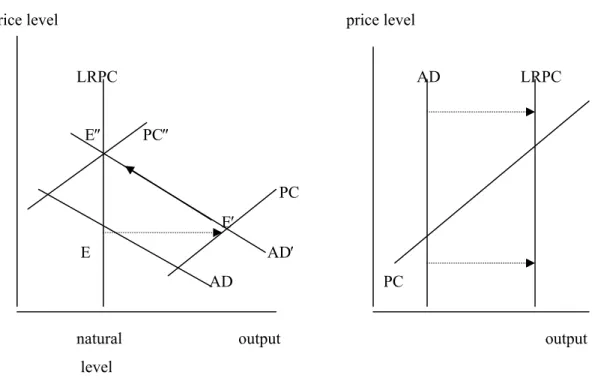
The simplest synthesis is to consider changes in public spending or the nominal money supply and assume expected inflation is zero. In that case, aggregate demand (AD) increases with real money balances and thus decreases with the price level. Inflation follows from a Phillips curve (PC) and increases if output is above its natural level. Figure 1(a) then shows that a fiscal or monetary expansion raises output in the short run (move from E to E′). This exerts upward pressure on nominal wages and prices and erodes the real value of money balances, so that the interest rate rises and the initial gains in aggregate demand are gradually dissipated. The upward shift of the Phillips curve thus moves the economy back along the aggregate demand schedule (from E′ to E″). In the long run there is only an increase in the price level, since the initial expansion of employment and output is fully dissipated by the real balance effect. Some die-hard Keynesians insist on a liquidity trap and deny that there is a real balance effect (i.e., bonds and money are perfect substitutes). In that case, the aggregate demand schedule is vertical and only fiscal expansion can get the economy back to full employment – see Figure 1(b).

Figure 1: Keynesian-classical synthesis and the real balance effect

(a) With real balance effect (b) Without real balance effect

price level price level

LRPC AD LRPC E″ PC″ PC E′ E AD′ AD PC

natural output output level

4.1. The Phillips curve and the accelerator hypothesis

Friedman (1968) and Phelps (1967, 1968) argue that the long-run Phillips curve is vertical at the natural unemployment rate or NAIRU, so that inflation increases (decreases) forever if unemployment is below (above) its natural rate. The short-run Phillips curve displays a

trade-off between inflation and unemployment. To illustrate, consider the accelerator Phillips-curve where next period’s inflation πt+1 depends on the output gap yt and expected inflation equals

last period’s inflation:

(1) πt+1 = πt + α yt + επ t+1 with α > 0, επ t ∼ IN(0,σπ2),

where επ t is a cost-push disturbance. Systematic deviations from the NAIRU (yt>0) induce a

never-ending spiral of inflation or deflation. Alternatively, aggregate supply increases with unexpected inflation. Aggregate demand depends negatively on the real interest rate:

(2) yt+1 = λ yt - β ( it - πt+1t - r) + εy t+1 = λ′ yt - β ( it - πt - r) + εy t+1

with 0<λ<1, λ′≡λ+αβ>λ, β>0 and εy t∼ IN(0, σy2),

where r denotes the long-run average real interest rate, λ gives persistence in the output gap and εyt is a demand shock (e.g., a fiscal expansion or animal spirits). The one-period-ahead

private-sector inflation forecast and the real interest rate are, respectively, πt+1t = πt + αyt

and it - πt+1t = it - πt - αyt. Rudebusch and Svensson (1999) show that this model fits US data

fairly well - see also Judd and Rudebusch (1998). The central bank uses the nominal interest rate to minimise the asymptotic expected value of the intra-temporal welfare loss γt = (πt-π*)2

+ κ yt2, where π* is desired inflation and κ>0 the weight given to full employment (output)

targeting. The equilibrium level of employment and output is efficient, so the desired output gap is zero. We thus abstract from inflation bias induced by time inconsistency problems (Kydland and Prescott, 1977; Barro and Gordon, 1983). Optimisation yields the Taylor rule for the optimal nominal interest rate:

(3) it = r + π* + (1 + µπ) (πt - π*) + µy yt = r + π* + (1 + µπ) (πt+1|t - π*) + (λ/β) yt

with 0<µπ≡αξ/[β(κ+α2ξ)]<1/αβ, µy≡(λ′/β)+αµπ>0 and ξ≡ ½+½(1+4κ/α2)½≥1. The constant

in the Taylor rule for the optimal nominal interest rate equals the sum of the average real interest rate and target inflation. The optimal nominal interest rate rule (3) ‘leans against the wind’, since the central bank deflates (boosts) the economy by raising (lowering) the nominal interest rate if inflation and output are above (below) target. The central bank reacts more vigorously to the output gap if aggregate demand is more persistent. The reaction coefficient on the inflation gap exceeds unity. Taylor (1993) estimates it=4%+1.5(πt-π*)+0.5yt.

Rotemberg and Woodford (1997, 1999) provide other estimates of Taylor rules. The special case of strict inflation targeting (κ=0) gives ξ=1, µπ=1/αβ, µy=(1+λ′)/β and yields the

maximum reaction to the inflation and output gaps. More emphasis on output targeting (higher κ) reduces both reaction coefficients. The Taylor rule can also be expressed in terms of the one-period-ahead inflation gap forecast and the output gap.

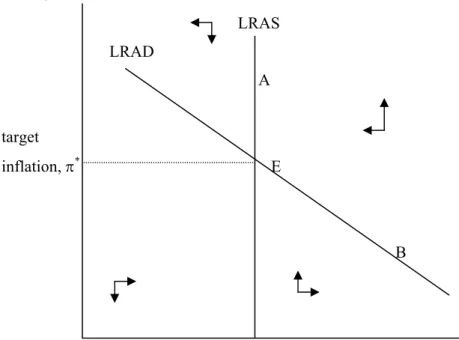
Substitution of (3) into (2) yields the closed-loop aggregate demand schedule:

(2′) yt+1 = - µy [α yt + β (πt - π*)] + εy t+1

which is portrayed together with the supply schedule (1) in Figure 2. Monetary disinflation (lower π*_{) temporarily pushes up the nominal interest rate, which lowers aggregate demand}

and output. An adverse shock to aggregate demand (lower εy) depresses unemployment,

which induces a looser monetary policy and lowers inflation. A permanent cost shock (higher

επ) induces inflation, which is combated with a tighter monetary policy. This induces

unemployment, so that stagflation results. Figure 2 illustrates the effects of these shocks.

Figure 2: Optimal inflation-output trade-off under the Taylor rule

Inflation LRAS LRAD A target inflation, π* _E B output

4.2. Battle of the mark-ups, pro-cyclical real wage and solvent policy rules

Layard, Nickell and Jackman (1991) in their empirical work allow for non-competitive wage setting and price setting and for conflict about the functional distribution of income. Their vision on the battle of the mark-ups allows for a pro-cyclical real wage, a quintessential Keynesian feature. Real wage rigidity arises from efficiency wages, which suggests that firms

pay above the market-clearing wage to recruit, motivate, discipline and/or retain workers. A reserve army of unemployed is thus an essential feature of a capitalist economy. Trade unions with monopoly power also negotiate a wage above the market-clearing level, particularly if labour demand and goods demand are fairly inelastic and firms make substantial monopoly profits. Real wage rigidity also occurs with insider-outsider behaviour and implicit contracts. Real wages usually rise in booms if unions are strong and fall during recessions. Price setting follows from monopolistic competition among firms. If the desired wage mark-up and the desired price mark-up (or profit margin) of firms are incompatible, inflation occurs in the short run (e.g., Rowthorn, 1977) and unemployment results in the long run. Inflation and eventually unemployment reconcile the conflict that arises if the claims of wage setters, price setters, the government and the rest of the world exceed the size of the national cake.

Consider the wage and price mark-up equations (same notation as section 2):

(4) p – (we _{+ t}

1 ) = α1 y + ε1, α1>0 and w – t2 - (pe + t3 ) = α2 y + ε2, α2>0

where ε1 represents price push (oil prices, import prices, firm monopoly power, etc.) and ε2

wage push (higher unemployment benefits, union power, etc.). With higher unemployment and lower output the power of firms and unions crumbles, so expected price and wage mark-ups fall. With we=w the price equation reduces to the downward-sloping labour demand schedule. Demand shocks then give rise to an unrealistic contra-cyclical real wage. Layard, Nickell and Jackman (1991) assume that wage and price surprises are the same (w-we=p-pe) and expected inflation is last period’s inflation. They thus obtain the following accelerator Phillips curve:

(1′) ∆π = α (y – y*_{), α≡ (α}

1 + α2)/2 > 0, y*≡ (ε1 + ε2+t)/(α1 + α2) >0

where y* _{denotes the difference between the distorted and the first-best level of equilibrium}

output. Distortions arise from price push, wage push and taxation, particularly if the degree of real wage rigidity (i.e., (α1 + α2)-1) is substantial. Changes in inflation rates capture policy

surprises, i.e. differences between actual and expected inflation rates, which induce higher unemployment. Employment and output are boosted, because employers and employees are fooled to think that prices, wages or taxes are lower than they actually are. Inflation and unemployment are influenced by a range of demand and supply factors. The short-run impact of incompatible claims on the national income is felt on inflation and the long-run impact on unemployment. The real consumption wage resulting from the battle of the mark-ups is:

Typically, wages are more responsive to output and unemployment than prices (α1<α2),

especially under the normal cost-pricing hypothesis. If output is above its natural rate, inflation rises. The resulting nominal price and wage surprises boost the real wage at the expense of the mark-up of firms in the short run. Rising (unanticipated) inflation reconciles claims on the national cake by cheating both firms and workers out what they intended. If α1<α2, this

redistributes income from firms to workers so that the real wage moves pro-cyclically.

With an aggregate demand schedule and a welfare loss function depending on squared deviations of output and inflation from their natural rates, one can derive contra-cyclical stabilisation rules for budgetary and monetary policy. Such optimal rules abstract from solvency and the intertemporal government budget constraint. To allow for a marriage of optimal stabilisation policy and tax and seigniorage smoothing (Barro, 1979; Mankiw, 1987), the counter-cyclical policy rules must be augmented with a constant factor to ensure solvency of the public sector (van der Ploeg, 1995). Principles of public finance require that tax rates and monetary growth go up and down together to equalise the marginal distortions of the various sources of public revenue. In contrast, stabilisation requires tax and monetary growth to move in opposite directions. For example, to boost employment one can either lower taxes or raise monetary growth. There is thus a tension between public finance and stabilisation objectives.

With flexible wages and prices higher permanent public spending is financed by a permanent increase in tax rates and monetary growth. With sluggish prices and wages the government counteracts short-run overheating of the economy with temporary cuts in monetary growth and tax hikes. Tax and seigniorage revenues are not smoothed over time. Instead, the tax hikes are sufficiently large to permit the government to pay off debt (or build up assets). To be able to finance principal and interest, the economy must eventually end up with higher inflation and monetary growth than with price and wage flexibility. Higher government commitments thus induce higher long-run inflation and tax rates, and also higher long-run unemployment. Similarly, temporary budgetary shocks have permanent effects on inflation and unemployment (cf., hysteresis). The traditional rules of public finance, i.e., finance temporary increases in spending with debt and permanent increases with taxes, no longer hold. When prices and wages are sluggish, temporary and permanent hikes in public spending induce permanently higher debt levels with adverse long-run effects on inflation and unemployment. In the short run inflation and taxes move in opposite directions, but in the long run they move up and down together.

4.3. Overlapping wage contracts

Important features of collective wage negotiation contracts are that they are fixed in nominal terms, they remain in force for anything up to three years, and are staggered. This led Fischer (1977), Phelps and Taylor (1977) and Taylor (1979) to develop theories of overlapping wage contracts. The main implication is that firms do not want to adjust their prices and wages to move too much out of line with others. Consequently, nominal shocks do not fully translate in wages and prices, and have real effects even under rational expectations (cf., section 5). A critique of this overlapping wage contracts approach is that the timing of nominal wage adjustments is exogenous and that it does not always explain why wage setters find it rational to sign contracts that are not synchronised and lead to obvious inefficiencies.

4.4 Near-rational wage and price setting

Akerlof, Dickens and Perry (2000) point out a shortcoming of conventional Phillips curves with a given NAIRU: in recent years low and stable rates of inflation have coexisted with a wide range of unemployment rates. They also argue that the coefficient on expected inflation in the Phillips curve changes over time. It was low in the fifties and sixties, higher in the seventies, and lower afterwards. They consequently find that there is a trade-off between inflation and unemployment at low rates of inflation, but not such a trade-off at high rates of inflation. It is not so important how people form expectations, but how they use them. Psychologists teach us that people use simple mental frames or decision heuristics and make cognitive errors. This suggests that people edit information and only react once a threshold of salience is passed. People thus ignore inflation if inflation is low at the time of setting wages and prices and that they need not project all of anticipated inflation. Furthermore, people ignore the usual links stressed by economists. For example, workers realise that inflation erodes their real purchasing power but forget, especially if inflation is low, that inflation increases the demand for their earnings or what they could earn elsewhere. In that case, prices and wages will be set lower than what economists typically predict. Wage earners thus systematically underestimate the effects of inflation on profits and the wages their employers are prepared to pay. Although at high rates of inflation a NAIRU will prevail, there may be substantial long-run gains in employment from moderate rather than from very low or zero inflation even if only a fraction of wages and prices are influenced by near-rational behaviour.

4.5. ‘Keynesian’ demand management and catching up with the Joneses

Consumer externalities like catching up with the Joneses have drastic implications for intertemporal macroeconomics. Since households do not internalise these external effects, they engage in a rat race to keep up consumption and competitive markets fail to yield the first-best outcome. Ljungqvist and Uhlig (2000) have no redistributive taxation, a balanced

government budget, a linear production technology with productivity shocks approximately following an AR(1) process, and utility depending negatively on labour supply and positively on the deviation of consumption from its aspiration level (a weighted average of past average consumption levels). Households consume a lot if the aspiration level of consumption is high, the tax rate is low, productivity is high and their dislike of work is low.

Ljungqvist and Uhlig show that a pro-cyclical tax on labour is required to restore the first-best outcome in competitive dynamic equilibrium driven by technology shocks. The tax rate thus varies positively with productivity. In a boom households chase each other into a rat race where they work and consume too much, so the government steps in to end this rat race and cools off the economy by raising the tax. In contrast, in a depression the tax is cut to bolster consumption if households are caught together in a negative spiral. Despite a competitive, market-clearing general equilibrium framework, there is a role for contra-cyclical Keynesian demand management to correct for the external effects caused by catching up with the Jones’s. Although Ljungqvist and Uhlig (2000) obtain a pro-cyclical fiscal policy, all markets clear and their result is not really Keynesian at all. Since they have no involuntary unemployment and no sluggish price formation, their theory really belongs to the classical or real business cycle schools discussed in the next section.

5. The Lucas critique and New Classical macroeconomics

The Lucas (1976) critique of econometric policy evaluation changed macroeconomics completely. The perceived trade-off between inflation and unemployment in the seventies was illusory, because as soon as the government tries to exploit this trade-off private agents react and change their behaviour. In particular, governments soon realise that to gain jobs by raising inflation will be unproductive as agents update their expectations of inflation and demand higher wages. The net result is higher inflation, but no extra jobs. The upshot is that the NAIRU also determines the short run, but more fundamentally that macroeconomists can no longer neglect rational expectations and micro foundations. Economic policy must depend on ‘deep structural’ preference and technology parameters. The Lucas critique gave birth to the New Classical macroeconomics, but also fuelled much of the New Keynesian revolution.

5.1 Rational expectations and the neutrality of monetary policy

New Classical economists, in contrast to Keynesian economists, are optimistic about the market mechanism and wary of government intervention (Lucas, 1972, 1973; Sargent and Wallace, 1975). They invoke rational expectations to argue that only policy surprises matter. Any anticipated action of the government to stimulate demand by fiscal or monetary policy is seen through by private agents, so they immediately press for higher wages as compensation for the anticipated increase in prices. This renders demand policy ineffective: people cannot be fooled

systematically. Only unanticipated money matters. The New Classical policy neutrality result depends on rational expectations and all markets clearing instantaneously, thus ruling out overlapping wage contracts, small menu costs, etc. (see section 5). The result leaves open the possibility that anticipated fiscal policy influences the natural rate of output (e.g. through the tax wedge or the Mundell-Tobin effect). In this sense, policy neutrality is a "theoretical curiosum". Most Keynesians are happy to adopt rational expectations, at least as far as financial agents is concerned, but assume that markets do not clear immediately. Rational expectations do not preclude rigid prices. For example, Dornbusch (1976) uses this to explain that monetary disinflation induces overshooting of the exchange rate. Similarly, anticipated expansion of public demand financed by T-bills can induce a recession in the period before the policy is implemented. The fall in economic activity occurs due to the appreciation of the real exchange rate and the rise in the long interest rate (being an average of future short interest rates). Keynesians thus acknowledge that credible announcements of policy changes matter for the economy. The really important difference between the New Classical and Keynesian economists is whether the market mechanism functions properly or not.

5.2. Real business cycles

Real business cycle economists extend the classic Ramsey model of economic growth to allow for stochastic technological shocks and study its impulse responses. The major achievement of Kydland and Prescott (1982) and other real business cycle economists is that technological shocks alone can in such calibrated competitive, dynamic general equilibrium models replicate the variability in and the various moments of US time series for production and consumption. Although calibration of such competitive models may replicate the business cycles of Western economies, this does not imply that these real business models are correct and that there are no other competing non-competitive models that can replicate the business cycle as well by relying on nominal demand shocks. Even real business cycle advocates suggest that 20 to 30 percent of cyclical output variability may be attributed to nominal shocks (e.g., Prescott, 1986; Shapiro and Watson, 1988; Aiyagari, 1994). Real business cycle models suffer from a lack of internal propagation. They have been extended in many ways to explain various empirical puzzles to do with employment variability and the excessive pro-cyclical nature of the real wage, and to allow for open economies. In particular, the economics based on the New Keynesian Phillips curve extends these models with imperfect competition on goods and labour markets and price and wage rigidity (see section 6). The real business cycle methodology is thus widely accepted nowadays. For a textbook exposition see Heijdra and van der Ploeg (2002, Chapter 15).

5.3. Getting macroeconomic priorities right

In a provocative paper Lucas (2003) surveys the evidence and argues that the gains from fine-tuning public spending and short-run management of aggregate demand are tiny compared with the large welfare gains from better long-run, supply-side, growth-promoting policies. To eliminate all variability in consumption, households are prepared to permanently give up one-half of one-tenth of a percent of their consumption level if households have a unit coefficient of relative risk aversion. Even if relative risk aversion is as high as 4, they are still only prepared to permanently forego one-fifth of a percent of their consumption. In practice, some of the shocks are technological, as stressed by real business cycle economists, and macroeconomic stabilisation policy is never perfect. The potential gains of stabilisation policy may thus be a factor three or five less than 0.05 or 0.2 percent. If these are the gains from macroeconomic stabilisation policy, Keynesian demand management is to all practical purposes irrelevant.

However, the welfare cost of business cycles once we allow for heterogeneous agents, incomplete risk sharing, and the catastrophic nature of becoming unemployed may be much higher. In fact, Krusell and Smith (1998, 2002) focus on hand-to-mouth consumers and show with US data that getting rid of all aggregate risk yields one tenth of one percent of consumption. Although the costs for unemployed with little wealth may be very high, the average effects are surprisingly small. However, in Europe the probability of being hit by unemployment and bad luck is much higher for some than for others, so that with depreciating skills avoiding to get caught in long-term unemployment is important and the welfare cost of business cycles may be much higher. Also, the welfare costs of business cycles may jump up once the prevalence of pre-existing tax and non-competitive distortions are taken account of. This literature is perhaps more relevant to show the way for a unified study of social insurance (reallocating risks) and macroeconomic stabilisation (reducing the variance of shocks and risk) than as a critique of stabilisation policy along the lines of New Keynesian macroeconomics. Beaudry and Pages (2001) also find much higher higher welfare cost of business fluctuations. Furthermore, the welfare cost of business fluctuations may be two orders of magnitude greater due to the adverse effect on the rate of economic growth (e.g., Barlevy, 2003).

Galí, Gertler and López-Salido (2002) stress the ‘inefficiency gap’ for assessing the welfare cost of business cycles. I prefer to use the inverse of their ‘inefficiency gap’, the virtual tax t*_{. This equals the virtual tax on labour (i.e., the wedge between the consumer}

wage and the marginal rate of substitution between consumption and leisure or the wage mark-up) plus the virtual tax on firms (i.e., the price mark-up). In competitive economies the virtual tax is zero, but in non-competitive economies this tax is positive. With higher levels of economic activity and profits it is more attractive to incur the cost of acquiring and disseminating information and markets become more competitive (‘thick markets’) or to attack existing monopolies, hence mark-ups may behave contra-cyclical. The evidence

suggests that changes in the contra-cyclical wage mark-up substantially outweigh those in the pro-cyclical price mark-up. This implies that the virtual tax moves contra-cyclically. The unconditional expected welfare cost of business cycles as fraction of trend consumption equals Ωexp(t∞*)var(t*), where Ω is half the ratio of the producer wage bill to gross domestic

product. The loss is high if the variance of the virtual tax is high, that is if labour supply is relatively inelastic and risk aversion high. The loss is also high if the pre-existing distortion, i.e., the steady-state virtual tax, is high, since then the gains from raising employment are high. Calibration yields much higher welfare costs than Lucas suggests, namely 0.8 percent to 4.6 percent of trend consumption. Even these costs underestimate true costs, since they ignore costs from efficient fluctuations in consumption and the welfare costs from inflation variability it self. Canzoneri, Cumby and Diba (2004) extend Galí, Gertler and López-Salido (2002) to allow for capital formation with adjustment costs and empirically estimated rules for public spending and the nominal interest rate. They calibrate their New Keynesian (or better Neoclassical) model to US data and also calculate a much higher welfare cost of nominal inertia, namely the average household is willing to forsake one to three per cent of consumption each period in order to avoid price and wage stickiness. This is twenty to sixty times as large as the loss suggested by Lucas (2003) and derives mainly from wage sluggishness. The estimated welfare losses are substantial, since the monetary authorities sub-optimally react to the difference between actual output and output in the non-stochastic steady state (rather than the first-best level of output under flexible wages and prices).

6. Micro-founded Phillips curves and welfare loss criteria

The New Keynesian Phillips curve assumes infinitely lived households, monopolistic competition among firms, staggered price setting and a competitive labour market. For a discussion of the forward-looking New Keynesian Phillips curve, see Roberts (1995), Clarida, Gáli and Gertler (1999), Galí (2003) and Woodford (2003). The sticky-information Phillips curve developed by Mankiw and Reiss (2002) develops an alternative where information about prices arrives in a staggered way to different firms. Most of the literature relies on the time-dependent mechanism for staggered prices put forward by Calvo (1983). The weakness of this practical approach is that this does not explain why such a mechanic form of price rigidity would be optimal. Future work on the New Keynesian Phillips curve may be based on state-dependent price resetting (e.g., Caplin and Leahy, 1991; Deveruex Engel, 2003).

6.1. The New Keynesian Phillips curve

Galí (2003) postulates a linear production function, a log-linear money demand schedule with unit income elasticity, and AR(1)-processes for productivity growth and demand shocks. Felicity depends on consumption (C) and hours worked (L), that is [Ct1-σ /(1-σ) – Lt1+ϕ /(1+ϕ)]

where σ is the coefficient of relative risk aversion and ϕ characterises the curvature of the dislike of work. He thus derives the New Keynesian Phillips curve:

(1″) πt = δπt+1 + α Et{yt+1} with α≡λ (σ+ϕ) > 0 and λ≡ (1-θ) (1-δθ)/θ > 0,

where 0<δ<1 is the utility discount factor and θ the fraction of firms that do not change their prices in a given period. With staggered adjustment of prices, firms care about their prices relative to those of other firms. Staggered pricing makes the overall adjustment of prices sluggish, even if individual prices change frequently. The reason is that no firm wants to be the first to up its price substantially. Inflation (1″) is, in contrast to the backward-looking Phillips curves (1) and (1′), determined in a forward-looking fashion. Inflation thus leads output. The reason is that firms realise that price stay put for some time and thus react to future demand and cost conditions. The sensitivity of inflation to the expected output gap (α) increases with the degree of relative risk aversion (σ) and the curvature of the dislike of work effort (ϕ), but decreases with the degree of price staggering (θ) and the discount factor (δ). With no staggered pricing (θ=0), there is a vertical aggregate supply schedule as the expected deviation from the first-best level of output is zero (i.e., Et{yt+1}=0). In general, changes in

mark-ups are the driving forces behind changes in aggregate inflation.

Rewriting the Euler equation for the consumer gives the dynamics of the output gap:

(6) yt = Et{yt+1} – [rt – Et{πt+1} - ρ]/σ

where ρ is the expected real interest rate (the discount rate plus terms that depend on budgetary policy and productivity growth). Expected growth in aggregate demand thus increases with the gap between the real and the expected interest rate, particularly if the elasticity of intertemporal substitution (1/σ) is large. Finally, the expected welfare loss resulting from departures from the first-best allocation written as a fraction of steady-state consumption equals:

(7) ½ (σ+ϕ) var(yt) + ½ (η/λ) var(πt)

where η>1 is the elasticity of substitution between consumer product varieties. The extraordinary achievement of New Keynesians is to derive a micro-founded expression for the welfare loss, which only depends on deep structural parameters (Woodford, 2003). Inflation in itself is not bad, but policy makers should worry about temporary distortions of relative prices. However, one should realise that the welfare loss (7) is derived under the

assumption that there is a subsidy on labour to exactly offset the virtual tax on labour due to monopolistic competition (i.e., log(η/(η-1)) ). This is unrealistic, since lump-sum taxes are not available and many governments need taxes on labour to fund a sizeable welfare state. In general, (7) should be modified to allow for pre-existing distortions and the separation of monetary policy from other public policies is not possible. The expression for the welfare loss is sensitive to the specification of the underlying model. For example, Erceg, Henderson and Levin (2000) also allow for staggered nominal wage contracts, which may be more realistic than staggered pricing. It is then not possible to restore the first-best allocation with flexible wages and prices and the welfare loss is augmented with a term that depends on the variance of wage inflation. The coefficient on that extra term rises with the elasticity of substitution between different varieties of labour and decreases with the degree of wage rigidity. Similarly, (7) suggests that the cost of price inflation rises with the elasticity of substitution between consumer goods varieties (higher η) and the degree of price rigidity (lower λ). A higher fraction of firms that do not change their prices in a given period (θ) implies a greater degree of price rigidity (lower λ and α) and thus a bigger welfare cost of inflation variability. With fully flexible prices there are no relative price movements and inflation does not bring any welfare costs. If labour and goods varieties are imperfect substitutes, they magnify the inefficient spread of output induced by staggered wages and prices and thus inflation variability causes greater welfare costs. The welfare cost of inefficient output fluctuations is particularly high if households relatively risk averse (high σ) and their marginal disutility of work varies a lot with employment variations (high ϕ).

With the New Keynesian Phillips curve the output gap driving inflation is precisely pinned down by micro foundations. Policy makers should target the deviation of output from the first-best level of output generated in the economy without price rigidities and not the deviation from some, arbitrary de-trended level of output. Rotemberg and Woodford (1999) and Woodford (2001) argue that the optimal output-response coefficient is much smaller if de-trended output is used instead of the theoretically correct more volatile output gap measure. Still, central bankers seem hesitant to target such a volatile target driven by technology and other shocks. Cukierman (this issue) argues that they may be right and gives a simple two-period example to demonstrate that sticky prices may in the absence of complete markets be superior to flexible prices. The target level of output may thus be distorted.

In two exciting papers Benigno and Woodford (2004a,b) derive a quadratic approximation to the micro-founded welfare loss function if there is a distorted steady state and no lump-sum taxes are available to finance a sizeable public sector. In that case, output and labour subsidies cannot be used to correct for monopolistic competition in product and labour markets in order to achieve the first-best optimum. They show that the central bank

must target a level of output that is distorted by taxes and monopolistic competition. Nevertheless, the optimal monetary policy only involves small deviations from zero inflation. The coefficients on the squared output and inflation gaps may in some extreme cases even be negative. Benigno and Woodford (2003) also abstract from lump-sum taxes and extend the analysis to allow for the joint determination of fiscal and monetary policies. Even though the extra instrument makes it easier to stabilise both output and inflation, there is ‘fiscal stress’ as the intertemporal government solvency condition needs to be satisfied (cf. Section 4.2).

Galí (2003) shows that with the New Keynesian Phillips curve a monetary expansion always expands output, but only generates a lower interest rate if risk aversion is sufficiently large and money growth is not too autocorrelated. The so-called liquidity effect is thus not necessarily the reason why output rises. In contrast to real business cycle theory, a positive technological shock is likely to lower employment in the short run unless monetary policy is sufficiently accommodating. Galí (2003) also argues at length in favour of simple Taylor rules reacting to the inflation g