Generating rules with predicates, terms and variables from the pruned neural networks

QUT Digital Repository:

http://eprints.qut.edu.au/

Nayak, Richi (2009) Generating rules with predicates, terms and variables from the pruned neural networks. Neural Networks , 22(4). pp. 405-414.

Generating rules with predicates, terms and

variables from the pruned neural networks

October 3, 2008

Abstract

Artificial neural networks (ANN) have demonstrated good predic-tive performance in a wide range of applications. They are, however, not considered sufficient for knowledge representation because of the incapability of representing the reasoning process succinctly. This pa-per proposes a novel methodologyGyanthat represents the knowledge of a trained network in the form of the restricted first-order predicate rules. The empirical results demonstrate that an equivalent symbolic interpretation in the form of rules with predicates, terms and variables can be derived describing the overall behaviour of the trained ANN with improved comprehensibility while maintaining the accuracy and fidelity of the propositional rules.

1

Introduction

Artificial neural networks (ANNs) have been successfully applied in many data mining and decision-support applications [6, 40]. The ability to learn

and generalise from data, that mimics the humans’ capability of learning from experience, makes ANNs useful for classification, regression and clustering tasks. However, ANNs are not considered sufficient for representation of knowledge due to poor comprehensibility of the results and the incapability of representing the explanation structures [38].

Previous researchers have overcome these shortcomings by transforming numerical weights of a trained network into a symbolic description known as Rule extraction. Several effective algorithms have been developed to ex-tract rules from a trained ANN into a propositional attribute-value language considering both of the decompositional and pedagogical rule-extraction ap-proaches [1, 8, 20, 36, 33]. The majority of them report that at least for several classification problems, it is worth extracting rules from neural works due to better predictive accuracy, in spite of the fact that neural net-works take much longer to train and rules are then generated at an additional computational cost in comparison to symbolic learners.

The sheer number of propositional rules generated by rule-extraction tech-niques is sufficient for some applications, but for many, this often makes the comprehension difficult. A means to generate fewer general rules that are equivalent to many more simple propositional rules is necessary. The first-order rules with variables and predicates have a greater expressiveness in rep-resenting the network’s knowledge in comparison to propositional attribute-value rules [23]. The first-order rules allow learning of general rules as well as learning of internal relationships among variables. The difference can be illustrated by the following example. Suppose the task is to learn the target conceptwife(X,Y)defined over the pairs of peopleX andY representing the positive and negative concepts. Based on one positive example: (Name = mary, Married to = john, Sex = female, Wife = true) and a few negative

examples; a propositional rule learner will learn a specific rule, If (Name = mary) ∧ (Married to = john) ∧ (Sex = female) Then (Wife = true). Like-wise many such specific rules will be generated from other examples. The rule generator that allows predicates and variables in rules will learn a single general rule, If married to(X,Y) ∧ female(X) Then wife(X,Y), whereX and

Y are variables that can be bound to any person, such as bindingX as ‘mary’ and Y as ‘john’ in the above case.

The research body on rule extraction from feedforward neural networks has concentrated on representing the knowledge contained in a network with propositional logic [1, 2, 8, 18, 19, 20, 33, 36]. To our knowledge, researchers have yet to tackle the problem of expressing a network’s knowledge in more expressive langauge such as first-order predicate logic or a subset of this.

This paper presents a novel methodology Gyan1 _{for representing the}

knowledge gained by a trained ANN with restricted first-order rules (contain-ing variables, finite terms and non-recursive predicates). The methodology first uses an existing propositional rule-extraction method to express ANN’s knowledge in propositional rules. These specific relationships are then impli-cated into generic predicate rules with variables and terms by applying the Plotkin’s ‘θ-subsumption rule of generalisation’ (or the least general generali-sation (lgg) concept) [26, 27] and the Michalski & Chilausky’s ‘generaligenerali-sation inference rules’ [22]. The methodology also includes the identification of im-portant variables for rule-extraction by pruning unnecessary nodes and links from the trained ANN using the threshold pruning and the agglomerative hi-erarchical clustering method. A knowledge base equivalent to the network can now be used for high level inference that allows user-interaction and enables greater explanatory capability.

The contribution of this paper is two-fold: (1) the reduction of search space for rule extraction techniques by utilizing the proposed heuristically guided decompositional pruning algorithm; and (2) the generation of re-stricted first-order rules from the propositional rules utilizing the proposed generalisation algorithm based on the concepts of the least general general-isation [27]. The first-order predicate rules in this paper do not allow the recursively defined predicates and infinite terms.

The performance of Gyan is demonstrated using a number of real world and artificial data sets. The empirical results demonstrate that an equivalent symbolic interpretation in the form of predicate rules with variables can be derived that describes the overall behaviour of the ANN with good compre-hensibility and maintaining the accuracy and fidelity as propositional rules. There is an overall 75.33% and 60% reduction in terms of the total number of rules without any loss of accuracy and fidelity when propositional rules are generalized into restricted first-order rules for a pedagogical rule extrac-tion algorithm considering the networks without pruning and with pruning respectively over a number of data sets. These reduction figures correspond to 68.7% and 65.5% for a decompositional rule extraction algorithm. It can also be ascertained from the empirical analysis that pruning of the trained network significantly improves the comprehensibility of the rule-set. The comparison of Gyan with symbolic learners such as C5 [29] and FOIL [30] shows that Gyan performs better than symbolic learners when the data is sparse, heavily skewed, or noisy.

This paper is organized as follows. The next section relates the proposed approach with existing works. Section 3 introduces the Gyan methodology that includes the pruning algorithm and the predicate rule generation algo-rithm. The subsequent section discusses the empirical analysis of the Gyan

methodology. Section 5 discusses some of the emergent issues involved with

Gyan and its algorithmic complexity. Finally the paper is concluded.

2

Related work

The motivation of the majority of rule extraction methods is understanding the decision process of the trained neural network. Many methods emerged in the last decade to express the decision process in propositional ground form rules. [1] is a good survey report of these methods until 1995. [20]and [31] include a review on more recent techniques. While the majority of rule extraction methods represent the trained network’s knowledge in the form of propositional rules, there have been some attempts to express neural net-work’s knowledge in the form of fuzzy logic [11], in the form of regression rules [32] and as finite-state automata for recurrent neural networks [16]. [38] emphasizes the need of generating other explanation structures such as rules with predicate and variables to provide more explanation power to neural networks. Also, there exists a need of good comprehensible rule-set generated from a neural network for allowing the adoption of ANNs in the real-world data mining problems where high emphasis is on understanding of the decision process [14]. The initiative to explain a neural network’s de-cision process as the rules containing predicates and variables in this paper is a step forward in this direction.

The primary advantage of the restricted first-order predicate rule repre-sentation used in this paper (with the lack of recursively defined predicates and infinite terms) is that implication is decidable [4] as well as it is appro-priate for real-life problems [21]. The advantage of using ANNs to extract predicate rules from data is that the hypothesis is not expressed in

first-order logic format and concepts are not found in an infinite search space as compared to FOIL or other first-order logic learners [30]. Using a first-order language for the expression of hypotheses, many problems such as match-ing or testmatch-ing for subsumption become computationally intractable and even the very notion of generality may acquire more than one meaning [26, 10]. Additionally, due to the rapid growth of utilizing decision making process in common use, it is highly desirable that a neural network based model should help users to pose their queries in order to retrieve the information that they are really interested in. Gyan opens up the possibility of interacting with data sets and neural networks by allowing the user to ask queries via the interface of a connectionist reasoning system.

Some of the rule extraction methods [39, 34] have utilized pruning to eliminate the trained network’s redundant connections and then cluster the hidden unit’s activation values to extract more accurate and comprehensible rules from networks. In the same line, the proposed method employs a prun-ing algorithm based on clusters of weights for reducprun-ing the search space for a rule extraction method. The majority of pruning algorithms require iterative training of the network after removing links or nodes [17, 35]. More often, the amount of computation necessary for retraining is much higher than that needed to train the originally fully connected network [7]. The pruning al-gorithm presented in this paper labels all unnecessary links according to the classification accuracy and removes the superfluous links all at once. This avoids the need of iterative training during the pruning process. The reduced search space now decreases the complexity of rule extraction techniques that face the problem of having a large search space to generate rules. Although the heuristics involved in the rule extraction methods obviate the need for enumerating all possible examples in the problem space, or limit the size of

the search for rules through weight space, pruning further reduces the search space. The primary objective of this paper is on the process of converting propositional rules into (restricted) first-order predicate rules. The pruning step is included to improve the efficacy of the rule generalisation process, another pruning algorithm can also be used.

In parallel to connectionist (neural networks) methods, many symbolic machine learning methods have been proposed emphasizing the learning of heuristic, deterministic and deductive models. R. J. Popplestone [28] first introduced the idea that the generalisation of literals exists and is useful for induction. Plotkin [26, 27] then rigorously analysed the notion of gen-eralisation to automate the process of inductive inference. He examined the properties of first-order clauses under subsumption and developed an al-gorithm for computing the least general generalisation of a set of clauses. The proposed methodGyan utilises theθ-subsumption rule of generalisation [26, 27] and the generalisation inference rules proposed by Michalski & Chi-lausky’s [22] for providing neural networks a better explanation power. The proposed method combines the qualitative knowledge representation ideas of symbolic learners with the distributed computational advantages of connec-tionist models for representing the trained neural network’s knowledge into a better explanation capacity rules.

3

The

Gyan

Methodology

The primary objective of the Gyan methodology is to improve the compre-hensibility of the rule set generated from a trained neural network while maintaining the classification accuracy of the network. The methodology enhances the representation of the network’s knowledge by introducing

vari-ables, terms and predicates in the generated rule set. This novel process of generating predicate rules is independent of any network architecture and can be applied to a set of propositional expressions. The methodology has two main steps. The first step includes pruning of the trained network such that only necessary input nodes, hidden nodes and links (connections) are left in the network. The second step includes generalization of the proposi-tional rules, that are extracted from the network using existing proposiproposi-tional rule-extraction methods, into predicate rules with variables and terms.

3.1

Pruning a feedforward neural network

The Gyan methodology is independent of the underlying feedforward net-work architecture. The constructive training technique such as cascade cor-relation [13] is utilized to dynamically build the neural networks. The cascade correlation algorithm adds new nodes with full connectivity to the existent ANN (including input nodes) as required. After the training converges, links between the hidden/output nodes and unimportant input nodes may still carry non-zero weights. These superfluous non-zero weights, though usually small, make the interpretation of neural representation difficult. In order to derive a concise set of symbolic rules, the input space is reduced by elimi-nating all unnecessary nodes and links from the network after the training is completed (minimum training and validation error).

Figure 1 outlines the heuristically guided decompositional pruning algo-rithm. The algorithm starts by grouping the incoming links for each non-input node in the network. The algorithm applies a metric-distance based agglomerative hierarchical clustering method to find the best n-way parti-tions [5]. This clustering method uses a bottom-up strategy that starts by placing each link (weight) in its own cluster, and then successively merges

clusters together until the inter-cluster distance is more than the default (or threshold) metric-distance. The algorithm then tests the groups of weighted links, labels them if they are unimportant based on two conditions 1.2 and 1.3 in Figure 1. The links are deleted only if both conditions are met.

The motivation behind the grouping of similar weights is that an indi-vidual link does not have a unique importance and the groups of similar links form an equivalence concept (not necessarily a rule) [39]. It also re-duces the computational complexity by testing a group of links to form a possible cluster instead of testing each individual link in the network. The performance of pruning depends upon the resultant clusters and the process of clustering largely depends upon the selection of metric-distance. It has been ascertained from the empirical analysis (as shown in section 4) that a smallmetric-distance in the range of 0.1 and 0.25 performs a good clustering solution leading to a better pruned network. The selection of the metric distance is discussed in more detail in Section 4.

A reason for requirement of a smaller metric-distance is that a penalty term has been added to the error function during training. This ensures that the minimal number of weights are generated and the weights are easily separated into groups. The modified cost function [41] is the sum of two terms based on the rectangular hyperbolic function:

θ(S, w) = X

p∈S

(targetp−actual outputp)2+λ∗

X i,j w2 ij 1 +w2 ij

The first term is the standard sum squared error over a set of examples

S. The second term describes the cost associated with each weight in the network and is a complexity term. The cost is small when wij is close to

zero and approaches unity (times λ) as the weight grows. Initially λ is set to zero and gradually increased by small steps until learning improves. The

learning rule then updates weights according to the gradient of the modified cost function with respect to the weights. The updated weights [41] are:

wij =wij + ∆wij −decay term

decay term=λ∗ 2wij

(1 +w2

ij)2

The decay term allows smaller weights to decay faster as compared to larger weights. The fundamental consideration behind this constraint is to generate the networks with weight values that are clustered into a number of small groups, instead of generating uniformally distributed weights.

The first testing to eliminate unnecessary links, input and hidden nodes from the trained network while preserving the classification accuracy of the network is based on the threshold pruning. The idea is that links with suf-ficiently low weights (|Pweights| < Bias) are not decisive for a node’s activation state, and are not contributing towards the classification of any of the examples. Many rule extraction methods are based on this theory that if the total sum of the weighted inputs exceeds the bias for a node then the ac-tivation of a unit will be near one and inputs that cause|Pweights|> Bias

should only be considered for rule extraction [39]. Consequently, the low weighted links (|Pweights|< Bias) are deemed unimportant for symbolic rules and can be ignored while extracting rules from network. The second testing is conducted for assessing the classification accuracy of the network by presenting each training example while setting the weight of these links as zero independently for each cluster. Only if the network’s classification do not change, the cluster is marked as unimportant. These two-fold provisions (steps 1.2 and 1.3 in Figure 1) assures that the network is not over-pruned and the predictive accuracy of the classification network is maintained. In the end of the pruning process, links that do not carry higher amount of

1. For each non-input node in the network:

1.1 Group the incoming links of similar weights in clusters adapting the hierarchal agglomerative clustering approach;

1.2 For each cluster:

1.2.1 Set the weight of each link to the average weight of that cluster; 1.2.2 If bias >cluster’s total weight then

the cluster is marked as unimportant;

1.3 Sequentially present all training examples to the network. For each training example:

1.3.1 For each cluster:

• Set all link weights to zero;

• Label the cluster as unimportant if there is no change in the network’s classification prediction

• Adjust the relevant weights to previous values.

1.4 Mark the cluster unimportant only if results from steps 1.2 and 1.3 agree. 2. For each non-output nodeni in the network:

2.1 Delete the links labelled as unimportant;

2.2 Ifall links of ni are labelled as unimportant then delete ni;

2.3 Remove ni if there are no output links from it.

3. Train the remaining nodes and links to satisfaction. Figure 1: The pruning algorithm

weights and nodes that do not have outgoing links are eliminated from the networks. As a result, the pruned network may have error rates higher than the network at the beginning of the pruning process. The pruned network is further trained using the quick-prop algorithm [12] until an acceptable error rate and classification accuracy are achieved.

3.2

Generating predicate rules from the network

The next step is interpretation of the knowledge embedded in the pruned network as symbolic rules. A rule set in the form of propositional ground expressions is first extracted from a trained ANN using the existing methods. The proposed predicate rule generation algorithm is presented in Figure 2 that implicates the specific relationships into generic rules with predicates and variables. This algorithm utilises the Plotkin’s ‘θ-subsumption rule of generalisation’ (or least general generalisation (lgg) concept) [26, 27] and the Michalski & Chilausky’s ‘generalisation inference rules’ [22] in the generali-sation task [25].

The generalisation task is to find a rule set represented in the subset language of first-order logic such that KR+ _{|= C}+

1 ∨...∨Cn+ and KR− |=

C₁−∨...∨C−

n, whereKR+ andKR− are knowledge representations that cover

all positive (C+

i ) and negative (Ci−) conjunctive expressions respectively. The

inferred knowledge representation uses the same definitions of predicates and terms as those in first-order logic except that terms are function free. The explicit negation of predicates is allowed in describing the goal concepts to avoid ‘negation-by-failure’. A fact is an instantiated/ground predicate if all variables are constant.

The following generalisation inference rules [25] are used to generate pred-icate rules from propositional rules:

θ-subsumption [27]: A clauseC θ-subsumes (¹) a clauseD, if there exists a substitution θ such that Cθ ⊆ D. C is known as the least general generalisation (lgg) ofD, andDis specialisation ofC ifC¹Dand, for every other E such thatEθ ⊆D, it is also the case thatEθ⊆C. The definition is extendible to calculate the least general generalisation of a set of clauses. The clause C is the lgg of a set of clauses S if C is the generalisation of each clause in S, and also a least general generalisation. Counting arguments [22]: The constructive generalisation rule generates the inductive assertions during learning that use descriptors, origi-nally not present in the given examples. The count quantified vari-ables rule generates descriptors #V cond, representing the number of

Vi that satisfy a condition cond, if a concept descriptor is in the form

of ∃V1, V2, .., Vl ·p(V1, V2, .., Vk). The count arguments of a predicate

rule generates new descriptors #V cond, by measuring the number of arguments in the predicate that satisfy a conditioncond, if a descriptor is a predicate with several arguments, p(V1, V2, ..).

Turning constants into variables: If a number of descriptions with dif-ferent constants are observed for a predicate or a formula, these obser-vations are generalised into a generic predicate or formula. E.g., if a unary predicate (p) holds for various constants a, b, ..l then the predi-cate p can be generalised to hold every value of a variable V with V

being either of a, b, ..l.

Term-rewriting: This reformulation rule transforms compound terms in elementary terms. Letpbe ann-ary predicate, whose first argument is a compound term consisting of t1 and t2, and the n−1 arguments are

p(t1∨t2, A)↔p(t1, A)∨p(t2, A) p(t1∧t2, A)↔p(t1, A)∧p(t2, A)

The ‘term-rewriting rule of generalisation’ is used to transform the con-junctive expressions into ground facts. If a concon-junctive expression contains only one value per attribute, it results in one fact, and if a conjunctive ex-pression contains more that one value for an attribute, it results in multiple facts. Minimisation procedures, such as the removal of duplicated instances of facts,removal of specific facts by more general ones andremoval of redun-dant entities in compatible facts-same predicate symbol and sign, are applied to remove the redundant facts or entities in facts. The fact definitions are utilised to express specific rules. These specific rules can now be expressed as clauses (disjunction of literals) by applying the logical equivalence law,

P ⇒Q≡ ¬P ∨Q.

To compute the generalisation of two clauses, literals must represent each possible mapping between the two clauses. The mapping is done by forming a set of pairs of compatible literals (i.e. the same predicate symbol and sign) from the two clauses (in the same way as is done for Plotkin’s concept of

selection [27, 42]). The set of selections of two clauses C1 = {l1, .., lk} and

C2 ={m1, .., mk}is defined as:

S(C1, C2) :={(li, mj)|∀li ∈C1∧mj ∈C2∧compatible}.

The lgg of two literals is computed before the computaion of lgg of two (function free) terms for computing the least general generalisation (lgg) of two clauses. The lgg of two clauses C1 and C2 is defined as:

lgg(C1, C2) = lgg(S(C1, C2)) =lgg(T emp(l1, .., lk), T emp(m1, .., mk))

lgg(l1, m1) =p(lgg(t1, s1), ..,(tn, sn))

A substitution θ = {X/t1, X/t2} uniquely maps two terms to a variable

1. Search for a DNF expression equivalent to the neural network. 2. Generate a single-depth type-hierarchy by input-space mapping,

with attributes as concepts, and values as sub-concepts.

3. Perform a symbol mapping of predicates to convert each conjunctive expression into a ground fact (such as Nodename#1 #2, hidden1 1

or output1 2, or simply p 1, p 2, .., p n).

4. Utilise the fact definitions to create specific clauses (clauses with constants,

C1,C2,..,Cn).

5. For all specific clauses do

5.1 Search for any two compatible clauses C1 and C2.

Let C1 ≡ {l1, .., lk} and C2 ≡ {m1, .., mk}

where each li, mi has same predicate and sign.

5.2 If such a pair C1 and C2 exists do

5.2.1 Determine a set of selections, S(C1, C2) :={(l1, m1), ..,(lk, mk)}

5.2.2 Compute a new word symbol to hold the two k-ary predicates

word1 :=T emp(l1, .., lk),word2 :=T emp(m1, .., mk)

5.2.3 let θ1 :=∅, θ2 :=∅, q1 :=word1 and q2 :=word2

5.2.4 While q1 6=q2 do

• Search arguments ofq1 and q2

• find t1 ∈q1 and t2 ∈q2 such that t1 and t2 are occurring at the

same position in q1 and q2 and t1 6=t2 or one of them is a

variable.

• Replacet1 and t2 with a new variableX whenever they occur

in the same position of q1 and q2.

• Letθ1 :=θ1∪ {t1/X}, θ2 :=θ2∪ {t2/X}

5.2.5 A rule with predicates and variables is generated (word1 =q1σ1, word2 =q2σ2)

6. Returnthe knowledge representation consisting of rules in the subset language of first order logic, facts and a type-hierarchy.15

variable X, whenever they occur together in the same position. This ensures that θis the proper substitution of t1 and t2. The size of the set of selections

of two clauses C1, C2 can be at most i×j, wherei is the number of literals

inC1 andj is the number of literals inC2. In general the resulting lgg of two

clauses contains a maximum ofi×j literals, many of which may be redundant and can be reduced by applying the Plotkin’s equivalence property. The lgg of two incompatible literals is undefined [27]. If there is a rule in the original ruleset that does not have a pair with which to generalise this rule, it is not reduced but just mapped in the appropriate format.

3.2.1 An example of generalization

A well-known Monk1 problem [37] is used to illustrate the generalisation process of propositional rules into predicate rules. An instance is classified as monk if Head shape = Body shape, or Jacket color = red. The Monk1 problem is chosen as it is a selection and equity problem emphasizing the higher-order proposition such as(Head shape = Body shape). The remaining input space in the network after pruning is: Head shape ∈ {round, square, octagon}, Body shape ∈ {round, square, octagon}, and Jacket color ∈ {red}. The propositional rule-extraction algorithm, RulVI[18], is applied for ex-tracting the knowledge of the ANN in propositional ground form. The DNF (disjunctive normal form) expression representing the output node having high output is:

1. Head shape = round∧ Body shape = round ∨

2. Head shape = square ∧ Body shape = square ∨

3. Head shape = octagon ∧Body shape = octagon ∨

4. Jacket color = red ∨

5. Head shape = round∧ Body shape = square ∨

6. Head shape = round∧ Body shape = octagon ∨

7. Head shape = square ∧ Body shape = round∨

8. Head shape = square ∧ Body shape = octagon ∨

9. Head shape = octagon ∧Body shape = round ∨

10. Head shape = octagon∧ Body shape = square.

Each conjunctive expression is represented as a ground fact. The first three expressions having the same arguments are mapped to the same pred-icate symbol of monk1. They are monk1(round, round), monk1(square, square), and monk1(octagon,octagon). The fourth expression is inferred as

monk2(red). Likewise expressions 5 to 10 indicating a different category (low output) are mapped to the new predicate symbol of monk3 with their corre-sponding values.

Collecting dependencies among attributes (associated within facts), a con-cept definition of monk(Head shape, Body shape, Jacket color) or monk(X, Y, Z) is formed for the output node that becomes the consequent of rules. While mapping each ground predicate to a rule, if a fact only contains a sub-set of these attributes then the consequent predicate is filled with variables in the missing arguments positions. The unique-name and domain-closure [9] assumptions are adopted that assert that the domain of discourse only in-cludes the attributes and their values explicitly mentioned in the problem domain. Each attribute is represented by a unique variable. In this example,

X denotes the Head shape attribute, Y denotes the Body shape attribute and Z denotes the Jacket color attribute. In other words, a constraint is im-posed on rules that the entity bound to the variableX must be a subconcept of Head shape for the inference to be valid.

1. monk(round, round, Z) ⇐monk1(round, round) 2. monk(square, square, Z) ⇐monk1(square, square) 3. monk(octagon,octagon, Z) ⇐ monk1(octagon,octagon) 4. monk(X, Y, red) ⇐ monk2(red)

5. ¬monk(round, square, Z) ⇐ monk3(round, square) 6. ¬monk(round, octagon, Z) ⇐monk3(round, octagon) 7. ¬monk(square, round, Z) ⇐ monk3(square, round) 8. ¬monk(square, octagon, Z)⇐ monk3(square, octagon) 9. ¬monk(octagon, round, Z) ⇐monk3(octagon, round) 10. ¬monk(octagon, square, Z) ⇒ monk3(octagon, square)

The important task now is to discover dependencies among arguments, introducing variables in rules based on the dependencies, and generalising them. This is done by finding thelgg of clauses. The generalisation algorithm presented in Figure 2 (step 5) iterates over the rules to find two compatible rules. Consider the compatible rules 5 to 10 to show the process of finding a lgg rule. On applying the logical equivalence law, P ⇒Q≡ ¬P ∨Q, rules 5 & 6 are transformed into:

1. ¬monk3(round, square) ∨ ¬monk(round, square, Z) 2. ¬monk1(round,octagon)∨ ¬monk(round,octagon, Z)

A new word symbol Temp is utilised to form the twok-ary predicates to hold the set of selections generated from the rules 5 and 6. Considering two choices for each antecedent, the set of selections of two rules contains a max-imum of 2n _{literals. These two clauses have two selections with consequent}

predicates.

1. Temp(¬monk3(round,square),¬monk(round,square,Z)) 2. Temp(¬monk3(round,octagon),¬monk(round,octagon,Z))

The θ-subsumption proceeds with the following steps: 1. Temp(¬monk3(round,Y),¬monk(round,Y,Z)) 2. Temp(¬monk3(round,Y),¬monk(round,Y,Z)) resulting in the inference rule:

• ¬monk(round,Y,Z)⇐monk3(round,Y) withθ= [Y/square] or [Y/octagon] This lgg rule is further θ-subsumpted with the rule number 7, and the same process of replacing arguments with variables is applied.

1. Temp(¬monk3(round,Y),¬monk(round,Y,Z))

2. Temp(¬monk3(square,round),¬monk(square,round,Z)) 1. Temp(¬monk3(X,Y),¬monk(X,Y,Z))

2. Temp(¬monk3(X,round),¬monk(X,round,Z)) 1. Temp(¬monk3(X,Y),¬monk(X,Y,Z))

2. Temp(¬monk3(X,Y),¬monk(X,Y,Z)) The resulting inference rule is:

• ¬monk(X,Y,Z) ⇐ monk3(X,Y) with θ = [X/round] or [X/square] and [Y/square]

This lgg rule is furtherθ-subsumpted with the rest of the compatible rules 8, 9 and 10 resulting in the following rule:

∀ X,Y,Z ¬monk(X,Y,Z) ⇐ monk3(X,Y).

Following the step 5 of the algorithm discussed in Figure 2, another in-ference rule based on the three compatible rules 1, 2 & 3 is found:

∀ X,Z monk(X,X,Z) ⇐ monk1(X,X).

The algorithm does not find any compatible rules for rule 4. Another rule is simply inferred as:

∀ X,Y,Z monk(X,Y,Z) ⇐ (Z == red).

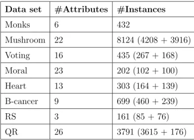
Table 1: Dimensionality of the data sets Data set #Attributes #Instances

Monks 6 432 Mushroom 22 8124 (4208 + 3916) Voting 16 435 (267 + 168) Moral 23 202 (102 + 100) Heart 13 303 (164 + 139) B-cancer 9 699 (460 + 239) RS 3 161 (85 + 76) QR 26 3791 (3615 + 176)

Monk1 problem domaini.e. the higher-order proposition that(Head shape = Body shape)(first two rules) rather than yielding each propositional rule such asHead shape = round and Body shape= round etc. This process results into significant improvement of comprehensibility with maintaining the accuracy of the propositional rules that are generalized and extracted from the trained neural network.

4

Empirical evaluation

4.1

Data sets

Table 1 lists the data sets that are used in this study providing information on the number of input variables and the number of total (positive + neg-ative) instances [24]. This includes two real-world data sets - Queensland Rail crossing safety (QR) and Remote Sensing (RS). The QR data set is an unbalanced data set (only 4.6% supporting the Risky cases) in which the

task is to identify Safe/Risky cases based on 26 attributes. The RS data is a multi-class problem in which the task is to recognize the existence of ur-ban, cultivated, forest and water areas from an image data. This paper only deals with the binary classification problem, as a result, each class is treated independently. The proposed approach can easily be adopted to nominal classification problems and is not restricted to binary classes. For example for a multiple-class outputs problem, rules with different consequent pred-icates can never subsume each other, the rules for each target concept are required to generate independently of one another. The rest of the data sets are selected from the UCI machine learning repository based on the fairly large number of attributes (Mushroom, Voting, Moral Reasoner etc), based on the variable domains (Cleveland heart disease (Heart) - continuous-valued problem domain) and benchmark data sets of Monks (Monk 1, 2, & 3).

4.2

Experimental setup

Two repetitions of the 10-fold cross-validation experiments are conducted. The results of the experiments are reported in Tables 2 to 6. Each value is an average from 20 networks or 20 rule-sets on the test data sets.

The performance of predicate rules inferred by Gyan is compared with the propositional rules extracted by two rule-extraction methods LAP[19] and RulVI[18]. These two methods represent each of the two rule extrac-tion categories [1]: decomposiextrac-tional or local (LAP) and pedagogical or global (RuleVI). Results are also compared with the symbolic propositional (decision-tree) rule learner C5 [29] and the symbolic first-order predicate rule learner FOIL [30]. In both FOIL andGyan, the ideas of both propositional and rela-tional learners are incorporated and rules are expressed in a restricted form of first-order logic (function-free predicates). The expressiveness of the rules

generated by FOIL however is better than that of the Gyan as the former supports iteration and recursion in its representation.

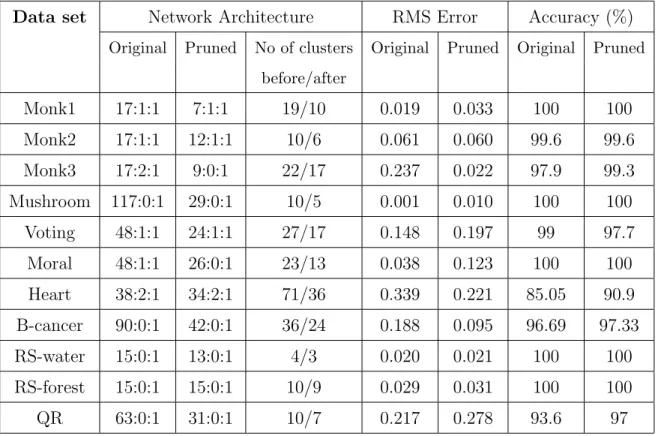
Table 2: Size, RMS error and classification accuracy of the networks

Data set Network Architecture RMS Error Accuracy (%)

Original Pruned No of clusters Original Pruned Original Pruned before/after Monk1 17:1:1 7:1:1 19/10 0.019 0.033 100 100 Monk2 17:1:1 12:1:1 10/6 0.061 0.060 99.6 99.6 Monk3 17:2:1 9:0:1 22/17 0.237 0.022 97.9 99.3 Mushroom 117:0:1 29:0:1 10/5 0.001 0.010 100 100 Voting 48:1:1 24:1:1 27/17 0.148 0.197 99 97.7 Moral 48:1:1 26:0:1 23/13 0.038 0.123 100 100 Heart 38:2:1 34:2:1 71/36 0.339 0.221 85.05 90.9 B-cancer 90:0:1 42:0:1 36/24 0.188 0.095 96.69 97.33 RS-water 15:0:1 13:0:1 4/3 0.020 0.021 100 100 RS-forest 15:0:1 15:0:1 10/9 0.029 0.031 100 100 QR 63:0:1 31:0:1 10/7 0.217 0.278 93.6 97

4.3

Networks training and pruning

Table 2 reports the architecture, root mean square (RMS) error and clas-sification accuracy of the networks before and after pruning. It also shows the number of clusters (groups of weighted links in the network) that are generated before pruning and the number of clusters that are remained after pruning. Since the inputs to the networks are sparsely coded, the number of nodes in the input layer is the total number of values of all attributes in

the data set. It is clear from the results that the pruning process results in removing superfluous links and nodes. It can also be observed from Ta-ble 2 (column 4) that the number of clusters is comparatively larger in the networks with hidden nodes, as the output node in the cascade networks receives activation from input nodes as well as hidden nodes. This is also a reason why a relatively smaller number of hidden units are required to learn a problem (column 2). The constructive technique such as cascade correla-tion [13] dynamically builds neural networks - the number of hidden nodes are incrementally added as they are needed - the initial architecture requires only input and output nodes to be defined. The classification accuracy is the ratio of correctly classified instances to the total number of instances on the test data.

The pruning algorithm includes the selection of ametric-distance param-eter which clusters the weights in trained ANNs to facilitate pruning. In general a small distance is required in the cascade correlation network so-lutions to group the individual links into a reasonable number of clusters. Many experiments are conducted to find a feasible range of the distance measure and setting a default distance. After many runs, it is found that when the distance is set between the range of 0.1 and 0.25, the pruned net-works yield the best combination of good accuracy and reduction in size. For example, the pruning process is most efficient when the distance is set as 0.2 for Monk1; 0.25 for Monk2; 0.1 for Monk3; 0.15 for Mushroom; 0.12 for Voting; 0.13 for Moral; 0.14 for Heart; 0.15 for B-cancer; 0.22 for RS; 0.14 for QR. The default distance is set as 0.15. When the distance between clusters is set to a larger value (say more than 0.3), each cluster normally contains the large number of elements which results in no reduction. The cumulative effect of such clusters is higher than the clusters with a lesser

number of elements towards the ANN’s prediction. The results in Table 2 confirm that training with pruning often results in a better (less complex) ANN than training without pruning, and only rarely results in worse ANNs. The further analysis of weight-clusters reveals that the elements in a clus-ter rarely show the required relationships (dependencies) among themselves. For example, none of the clusters in the Monk1 problem domain directly show the logical relationship of Head shape = Body shape among its mem-bers. The non-dependencies among elements in a cluster shows the need of applying further analysis to the remaining network in order to represent the embedded knowledge in the form of symbolic rules.

4.4

Predicate rule performance

The quality of extracted rules is evaluated using the criteria of classification accuracy, fidelity and comprehensively as presented in [1, 24]. The classifica-tion accuracy is the percentage of data instances that are correctly classified by the extracted rules. Fidelity is a measure of the agreement between the pruned network and the extracted rule set for correctly classifying the in-stances. The comprehensibility of the propositional rule set is expressed by the number of conditions per rule and the total number of rules. The criteria is extended to include the comprehensibility of the predicate rule sets. It is measured as the number of entities per predicate, number of predicates per rule and the total number of rules in the generalized predicate rule-sets. Table 3 shows the details of the extracted ground form rules when the LAP rule extraction technique [19] is applied to networks without and with pruning labelled as ‘Original’ and ‘Pruned’ respectively. The last row in this table indicates the average performance over the data sets for which the LAP method was successful in extracting rules from both original and

pruned networks. This row also includes the average performance of rules inferred using C5 [29].

The LAP rule extraction technique decomposes the network into a col-lection of networks and extracts a set of rules describing each constituent network. The core idea in LAP is to isolate the necessary dependencies be-tween inputs and each non-input node in the network and form a symbolic representation for each node. This usually results in rule sets with high accu-racy and high fidelity but with larger number of rules. This can be observed in Table 3. A shortcoming of LAP and other decompositional techniques is that these methods become cumbersome when the search space is too large (in terms of number of attributes). In LAP, dimensionality of the search space is exponential in the number of values of all attributes, leading to a substantial gain when all attributes and values per attribute are not included in the search because of pruning. For example, LAP fails to extract rules from original networks for ‘Voting’, ‘Heart’ and ‘B-cancer’ data, on other hand, rules are successfully extracted from the pruned networks due to the reduced set of attribute-values (Table 3).

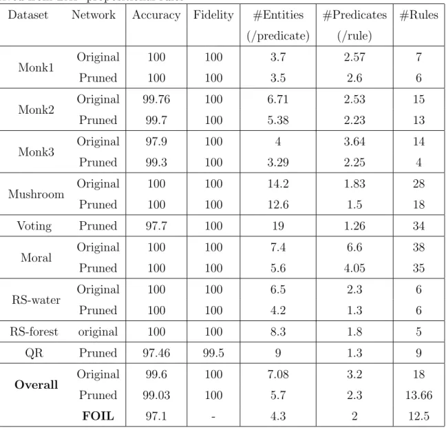
The LAP propositional rules are generalized into predicate rules. Ta-ble 4 shows the accuracy, fidelity, number of entities per predicate, number of predicates per rule and the total number of rules in the generalized pred-icate rule-sets for both original and pruned networks. Results in Tables 3 and 4 show that the generalization step does not have any information loss keeping the accuracy and fidelity maintained as it was for a propositional rule-set. There is a significant improvement in comprehensibility in terms of the reduced number of rules and predicates (conditions) in comparison to propositional rules. There is 68.7% and 65.6% reduction in terms of the total number of rules when propositional rules are generalized into predicate

Table 3: Accuracy, fidelity and comprehensibility of LAP propositional rules Dataset Network Accuracy Fidelity #Conditions #Rules

(%) (%) (per rule) Monk1 Original 100 100 3.5 18 Pruned 100 100 2.6 16 Monk2 Original 99.7 100 4.5 63 Pruned 99.7 100 3.4 59 Monk3 Original 97.9 100 4.8 48 Pruned 99.3 100 2.3 39 Mushroom Original 100 100 13.1 51 Pruned 100 100 10.3 36 Voting Pruned 97.7 100 9.7 86 Moral Original 100 100 5.1 156 Pruned 100 100 4.5 79 RS-water Original 100 100 4.7 9 Pruned 100 100 4.1 9 RS-forest Original 100 100 5.3 10 QR Pruned 97.46 99.5 1.8 27 Overall Original 99.6 100 5.95 57.5 Pruned 99.03 100 4.53 39.6 C5 98.99 - 2.05 9.27

Table 4: Accuracy, fidelity and comprehensibility of predicate rule sets de-rived from LAP propositional rules

Dataset Network Accuracy Fidelity #Entities #Predicates #Rules (/predicate) (/rule) Monk1 Original 100 100 3.7 2.57 7 Pruned 100 100 3.5 2.6 6 Monk2 Original 99.76 100 6.71 2.53 15 Pruned 99.7 100 5.38 2.23 13 Monk3 Original 97.9 100 4 3.64 14 Pruned 99.3 100 3.29 2.25 4 Mushroom Original 100 100 14.2 1.83 28 Pruned 100 100 12.6 1.5 18 Voting Pruned 97.7 100 19 1.26 34 Moral Original 100 100 7.4 6.6 38 Pruned 100 100 5.6 4.05 35 RS-water Original 100 100 6.5 2.3 6 Pruned 100 100 4.2 1.3 6 RS-forest original 100 100 8.3 1.8 5 QR Pruned 97.46 99.5 9 1.3 9 Overall Original 99.6 100 7.08 3.2 18 Pruned 99.03 100 5.7 2.3 13.66 FOIL 97.1 - 4.3 2 12.5

rules considering the networks without and with pruning respectively. Ad-ditionally, results also demonstrate that pruning significantly improves the comprehensibility of the rule-set by reducing the number of conditions (or predicates) per rule and the number of total rules in the rule-set. The av-erage (over all data sets) percentage improvements in extracting rules from the pruned network in comparison to the network without pruning are 0.9% for accuracy, 23.8% for #conditions per rule, 31% for #propositional rules, 19.5% for #entities per predicate, 28.1% for #predicates per rule and 25% for #predicate rules.

The propositional rule extraction technique RulVI[18] is also applied to networks to extract rules in propositional ground form. The motif of the

RulVI pedagogical rule extraction technique is that a conjunctive rule holds only when all antecedents in the rule are true and hence by changing the truth value of one of the antecedents the consequent of the rule changes.

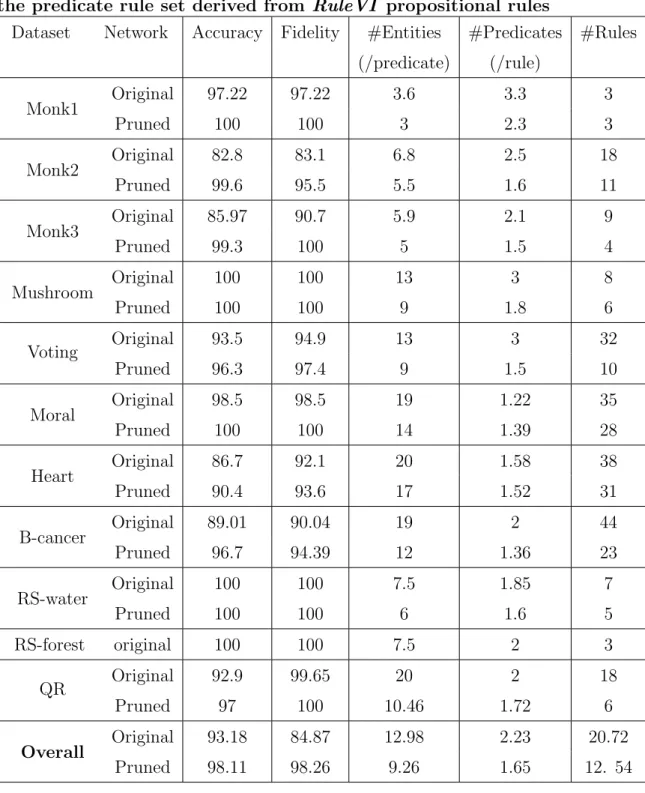
RulVI generates a rule set by repeatedly changing antecedents of the training instances, querying the trained ANN, and examining the network’s response. Tables 5 and 6 show the performance of the propositional and predicate rule sets respectively. The accuracy and fidelity of these rule sets are inferior to the rules sets reported in Tables 3 and 4 due to the pedagogical (or local) nature of the rule extraction. However, accuracy of the predicate rule sets is still maintained as the accuracy of propositional rule-sets. This asserts that the accuracy of the generated predicate rules very much depends on the rule-extraction algorithm that is employed to extract the propositional ground form rules from the trained ANN. The Gyan methodology enhances the expressiveness of the extracted propositional rules by introducing vari-ables and predicates in rules without the loss of accuracy or of fidelity to the ANN solution. The predicate rules mapped from the propositional rules are

Table 5: Accuracy, fidelity and comprehensibility of RuleVI propositional rule sets

Dataset Network Accuracy Fidelity #Conditions #Rules

(%) (%) (per rule) Monk1 Original 97.22 97.22 2.7 22 Pruned 100 100 1.9 10 Monk2 Original 82.8 83.1 5.76 130 Pruned 99.6 95.5 4.8 38 Monk3 Original 85.97 90.7 3.6 39 Pruned 99.3 100 1.92 13 Mushroom Original 100 100 16.6 24 Pruned 100 100 2.63 11 Voting Original 93.5 94.9 7.21 80 Pruned 96.3 97.4 4 30 Moral Original 98.5 98.5 5.41 43 Pruned 100 100 3.92 39 Heart Original 86.7 92.1 7.58 161 Pruned 90.4 93.6 7.55 116 B-cancer Original 89.01 90.04 8.01 274 Pruned 96.7 94.39 2.63 46 RS-water Original 100 100 1.93 16 Pruned 100 100 1.83 12 RS-forest original 100 100 2.7 55 QR Original 92.9 99.65 2.08 97 Pruned 97 100 1.83 12 Overall Original 93.18 84.87 6.17 84 Pruned 98.11 98.26 3.27 31.9

significantly less in numbers but maintain the quality as shown in Tables 4 and 6. There is a 75.33% and 60% reduction in terms of total number of rules when propositional rules are generalized into predicate rules for the RuleVI

algorithm considering the networks without and with pruning respectively averaged over all data sets. Tables 5 and 6 also show that the perfor-mance of rule sets is considerably improved when pruning is used to reduce the search space. The average (over all data sets) percentage improvement of extracting rules from the pruned network in comparison to the network without pruning is 5.3% for accuracy, 15% for fidelity, 47% for #conditions per propositional rule , 62% for #propositional rules , 28% for #entities per predicate , 26% #predicates per rule and 40% for #predicate rules.

These rule extraction results are related to the cascade correlation net-works, however, the similar performance is illustrated when networks are trained with the BpTower [15], back-propagation and CEBPN [3] networks. These results are not shown here due to the space constraint.

4.5

Comparative performance of

Gyan

with symbolic

learners

Performance of the Gyan methodology is also compared with C5 [29] and FOIL [30]. The last row of Tables 3 and 4 shows the average performance of C5 and FOIL (over all data sets) respectively. The Gyan approach yields better accuracy than symbolic learners. However, comprehensibility of the generated predicate rule-sets with using Gyan is inferior to those generated with using FOIL and to the propositional expressions generated with using C5. The generation of rules in C5 is based on data partitioning. The C5 algorithm generates a subset of solutions rather than a complete solution for

Table 6: The predictive accuracy, fidelity and comprehensibility of the predicate rule set derived from RuleVI propositional rules

Dataset Network Accuracy Fidelity #Entities #Predicates #Rules (/predicate) (/rule) Monk1 Original 97.22 97.22 3.6 3.3 3 Pruned 100 100 3 2.3 3 Monk2 Original 82.8 83.1 6.8 2.5 18 Pruned 99.6 95.5 5.5 1.6 11 Monk3 Original 85.97 90.7 5.9 2.1 9 Pruned 99.3 100 5 1.5 4 Mushroom Original 100 100 13 3 8 Pruned 100 100 9 1.8 6 Voting Original 93.5 94.9 13 3 32 Pruned 96.3 97.4 9 1.5 10 Moral Original 98.5 98.5 19 1.22 35 Pruned 100 100 14 1.39 28 Heart Original 86.7 92.1 20 1.58 38 Pruned 90.4 93.6 17 1.52 31 B-cancer Original 89.01 90.04 19 2 44 Pruned 96.7 94.39 12 1.36 23 RS-water Original 100 100 7.5 1.85 7 Pruned 100 100 6 1.6 5 RS-forest original 100 100 7.5 2 3 QR Original 92.9 99.65 20 2 18 Pruned 97 100 10.46 1.72 6 Overall Original 93.18 84.87 12.98 2.23 20.72 Pruned 98.11 98.26 9.26 1.65 12. 54

the given problem. This raises the issue of totality of knowledge vs. the comprehensibility of generated rule-sets. The extraction of total knowledge embedded within the trained ANNs adversely affects the comprehensibility of rules. The rule extraction algorithms search for the rules in the problem space that is approximated by the trained ANN for the given problem.

In general, Gyan performed (in terms of accuracy and comprehensibil-ity) better than symbolic learners when small amount of data (less than 100 patterns such RS-water and RS-forest) is available for training. This shows that neural network based techniques are better than symbolic learners when the large amount of data is not available. Gyan performed better than FOIL when the distribution of patterns among classes is uneven such as QR. Gener-alization accuracy of FOIL is worse thanGyan as shown by the performance on test datasets, in particular when the data has noise such as Monk3.

5

Discussion and algorithmic complexity

The comprehensibility of the propositional rule-set using a propositional rule extraction method is sometimes poor and does not serve the intended purpose of understanding the decision process. The Gyan methodology solves this problem by including the pruning algorithm to remove redundant inputs and by including the generalisation algorithm to generate a more compact form of rules. The restricted first-order predicate rules mostly result in a smaller, equivalent set of rules mapped from the pruned and trained network. This process is especially helpful when a data set contains relational attributes (functional dependent) as in the Monk1 problem domain. If the relevance of a particular input attribute depends on the values of other input attributes, then the generalisation algorithm is capable of showing that relationship in

terms of variables.

Most importantly, as shown in empirical evaluation, pruning improves the accuracy and comprehensibility of rule extraction from networks. For exam-ple, a shortcoming of LAP and other decompositional rule extraction tech-niques is that these methods become cumbersome when the search space is too large for an effort to produce high fidelity. Pruning allows these methods to only consider the parts of the search space whose elements are involved in approximating the target concepts. Similarly, pruning significantly reduces the number of amended instances to test the proposed rules by removing attributes that do not have any impact on the target concept. RulVI and other pedagogical methods usually extract rules by only ‘completely cover-ing’ the set of instances that are used to obtain them. Thus the complexity of such methods and of the extracted rules is also decreased with an increase in rule quality (comprehensibility, predictive accuracy, etc) by punning the superfluous links and nodes in the trained networks.

The algorithmic complexity of Gyan depends upon the core algorithms used in different phases. The steps in the pruning algorithm that consume most of the computational effort are clustering the network’s links of similar weights, labelling/eliminating unimportant clusters and training the remain-ing nodes and links. The initial clusterremain-ing step requiresO(u×l2_{) time, where} u is the number of non-input nodes in the trained network andl is the aver-age number of links received by a node. The cluster elimination step requires

O(n×u×l), where n is the number of training examples.

The generalisation algorithm requires O(l×m2_{), where l is the number}

of clauses according to the DNF expression equivalent to the trained neural network and m is the total number of attributes in the problem domain. Pruning of the network assists in significantly reducing the total number of

attributes. It can be observed from the description of the generalisation algo-rithm that the length of the resulting lgg of two rules C1,C2 can be at most

((|C1| × |C2|)) literals. One generalised literal is included in the lgg for each

selection, many of which may be redundant. Since Gyan is concerned with explaining the ANNs comprehensively, the number of generated lgg literals is not much of a concern. The generated DNF expression is constrained to a single-depth rule mapping (inputs to outputs). The body of a rule contains at most two literals (including consequent) to be generalised at any time. Even for a multiple outputs problem, rules with different consequent pred-icates can never subsume each other, the rules for each target concept are generated independently of one another.

The Gyan methodology pays a high price (in terms of computation) for the benefits of an improved explanation capability of the ANNs process. However, the use of reliable and general (portable and scalable) propositional learners can makeGyan more efficient. Moreover, an improved propositional rule extraction method effectively utilizing and extending the pruning algo-rithm to extract proposition rules such as [34] can further improve Gyan. Overall, providing an explanation in terms of rules including generic predi-cates is a step forward in the symbolic representation of networks.

6

Conclusion

This paper presents theGyan methodology which expresses the decision pro-cess of trained networks in the form of restricted first-order predicate rules. Even though ANNs are only capable of encoding simple propositional data, with the addition of the inductive generalization step, the knowledge repre-sented by the trained ANN is transformed into a representation consisting

of rules with predicates and variables. Empirical results show that a sig-nificant improvement in the comprehensibility of predicate rules is achieved while maintaining the accuracy and fidelity as of propositional rules extracted from the trained networks.

The successful application and competitive results obtained byGyan for various problem domains demonstrate its effectiveness in real-life problems (such as Queensland Rail and Remote Sensing), in fairly large size problems (in terms of number of attributes, such as Breast Cancer, Moral Reasoner, Voting and Mushroom), and in continuous-valued problem domains (such as Cleveland heart disease). The comparison of Gyan with symbolic learners such as C5 [29] and FOIL [30] shows that the comprehensibility of Gyan is inferior to them but the accuracy is superior to them . The empirical analysis also shows that Gyan performs better than symbolic learners when the data is sparse, heavily skewed, or noisy.

The development and success ofGyan shows that the propositional rule-extraction techniques can be effectively extended to represent knowledge em-bedded in trained ANNs in the form of first-order logic language with some restrictions. The logic required in representing the network is restricted to pattern matching for the unification of predicate arguments and does not contain functions. The Gyan methodology applies distributed connectionist networks (ANNs) at the lower level. In rule extraction step, it introduces the variables and relations to the symbolic rules eliciting the knowledge em-bedded within trained ANNs. At the higher level reasoning, this generic and conceptual knowledge can be represented in knowledge base reasoners and can provide user interface.

References

[1] Andrews, R., Diederich, J., and Tickle, A. A survey and critique of techniques for extracting rules from trained artificial neural networks.

Knowledge Based Systems 8 (1995), 373–389.

[2] Andrews, R., and Geva, S. Rule extraction from a constrained error back propagation mlp. In Proc. of 5th Australian Conference on Neural Networks, Brisbane, Australia (1994), pp. 9–12.

[3] Andrews, R., and Geva, S. Rules and local function networks. In

Rule and Networks (1996), R. Andrews and J. Diederich, Eds., Soci-ety For the Study of Artificial Intelligence and Simulation of Behaviour Workshop Series (AISB/32596), pp. 1–15.

[4] Bergadano, F., and Gunetti, D. Inductive Logic Programming: From Machine Learning to Software Engineering. The MIT Press, Cam-bridge, 1995.

[5] Berkhin, P. Survey of clustering data mining techniques. Tech. rep., Accrue Software, San Jose, California, 2002.

[6] Bishop, C., Ed. Neural Networks for Pattren Recognition. Oxford University Press, 2004.

[7] Blassig, R. Gds: Gradient descent generation of symbolic rules. In Advances in neural information processing systems, J. D. Cowan, G. Tesauro, and J. Alspector, Eds., vol. 6. Morgan Kaufmann, 1994, pp. 1093–1100.

[8] Bologna, G. Is it worth generating rules from neural network ensem-bles? Journal of Applied Logic 2, 3 (2004), 325–348.

[9] Brachman, R. J., Levesque, H. J., and Reiter, R., Eds. Pro-ceedings of first international conference on principles of knowledge rep-resentation and reasoning (1989), CA: M. Kaufmann.

[10] Buntine, W. Generalised subsumption and its applications to induc-tion and redundancy. Artificial Intelligence 36 (1988), 149–176.

[11] Castro, C. J., Mantas, C. J., and Benitez, J. M. Interpretation of artificial neural networks by means of fuzzy rules. IEEE Transactions on Neural Networks 13, 1 (2002), 101–116.

[12] Fahlman, S. E. Faster-learning variations on back-propagation: An empirical study. In Proc. of the 1988 Connectionist Models Summer School (1988), Morgan Kaufmann.

[13] Fahlman, S. E., and Lebiere, C. The cascade-correlation learn-ing architecture. In Advances in neural information processing systems, vol. 2. Morgan Kaufmann, 1990.

[14] Fayyad, U. Data mining and knowledge discovery. IEEE Expert 11, 5 (1996), 20–25.

[15] Gallant, S. I. Perceptron-based learning algorithms. IEEE Transac-tions on Neural Networks 1, 2 (1990), 179–191.

[16] Giles, C. L., Miller, C. B., Chen, D., Chen, H. H., Sun, G. Z., and Lee, Y. C. Learning and extracting finite state automata with second-order recurrent neural networks.Neural Computation 4, 3 (1992), 393–405.

[17] Hassibi, B., and Stork, D. Second order derivatives for network pruning: Optimal brian surgeon,. In Advances in neural information

processing systems, J. D. Cowan, G. Tesauro, and J. Alspector, Eds., vol. 6. San Mateo, CA: Morgan Kaufmann, 1994, pp. 164–171.

[18] Hayward, R., Ho-Stuart, C., and Diederich, J. Neural networks as oracles for rule extraction. In Connectionist System for Knowledge Representation and Deduction. Queensland University of Technology, Australia, 1997, pp. 105–116.

[19] Hayward, R., Tickle, A., and Diederich, J. Extracting rules for grammar recognition from cascade-2 networks. In Connectionist, Statistical and Symbolic Approaches to Learning for Natural Language Proc. Springer-Verlag, Berlin, 1996, pp. 48–60.

[20] Hruschka, E. R., and Ebecken, N. F. Extracting rules from mul-tilayer perceptrons in classification problems: A clustering-based ap-proach. Neurocomputing 70, 1-3 (2006), 384–397.

[21] Lavrac, N., Dzeroski, S., and Grobelnick, M. Learning non re-cursive definitions of relations with linus. InMachine Learning-EWSL’91

(1991), Y. Kodratoff, Ed., pp. 265–281.

[22] Michalski, R. S., and Chilausky, R. L. Knowledge acquisition by encoding expert rules versus computer induction from examples-a case study involving soya-bean pathology. International Journal of Man-Machine Studies 12 (1980), 63–87.

[23] Mitchell, T. M. Machine Learning. The McGraw-Hill Companies, Inc, 1997.

[24] Nayak, R. Gyan: A Methodology for Rule Extraction from Artificial Neural Networks. A data mining and machine learning approach. PhD thesis, Queensland University of Technology, Brisbane, Australia, 2001. [25] Nayak, R. Generating predicte rules from neural networks. In Pro-ceedings of the Sixth International Conference on Intelligent Data Engi-neering and Automated Learning (IDEAL), Brisbane, Australia (2005), pp. 234–241.

[26] Plotkin, D. G. A note on inductive generalisation. In Machine In-telligence, B. Meltzer and D. Michie, Eds., vol. 5. Edinburgh University Press, 1970, pp. 153–163.

[27] Plotkin, D. G. A further note on inductive generalisation. In Ma-chine Intelligence 6, B. Meltzer and D. Michie, Eds., vol. 6. Edinburgh University Press, 1971, pp. 101–124.

[28] Popplestone, R. J. An experiment in automatic induction. In Ma-chine Intelligence 5, B. Meltzer and D. Michie, Eds. Edinburgh Univer-sity Press, 1970, pp. 203–215.

[29] Quinlan, J. R. Induction of decision trees. Machine Learning 1, 1 (1986), 81–106.

[30] Quinlan, J. R. Learning logical definitions from relations. Machine Learning 5, 3 (1990), 239–266.

[31] Saad, E. W., and D, W. Neural network explanation using inversion.

[32] Saito, K., and Nakano, R. Extracting regression rules from neurakl networksneural network explanation using inversion. Neural Networks 15, 10 (2002), 1279–1288.

[33] Setiono, R. Extracting rules from prunned neural networks for breast cancer diagnosis. Articifical Intelligence in Medicine 8, 1 (1996), 37–51. [34] Setiono, R. Extracting rules from neural networks by pruning and

hidden-unit splitting. Neural Computation 9, 1 (1997), 205–225.

[35] Setiono, R. A penalty function approach for pruning feedforward neural networks. Neural Computation 9, 1 (1997), 185–205.

[36] Taha, I. A., and Ghosh, J. Symbolic interpretation of artificial neu-ral networks. IEEE Transactions on Knowledge and Data Engineering 11, 3 (1999), 448 – 463.

[37] Thrun, S., Bala, J., Bloedorn, E., Bratko, I., Cestnik, B., Cheng, J., Jong, K. D., Dzeroski, S., Hamann, R., Kaufman, K., Keller, S., Kononenko, I., Kreuziger, J., Michalski, R., Mitchell, T., Pachowicz, P., Roger, B., Vafaie, H., de Velde,

W. V., Wenzel, W., Wnek, J., and Zhang, J. The monk’s

prob-lems: A performance comparison of different learning algorithms. Tech. Rep. CMU-CS-91-197, Computer Science Department, Carnegie Mellon University, Pittsburgh, PA, 1991.

[38] Tickle, A., Andrews, R., Golea, M., and Diederich, J. The

truth will come to light: directions and challenges in extracting the knowledge embedded within trained artificial neural networks. TEEE Trans on Neural NEtworks 9, 6 (1998), 1057–1068.

[39] Towell, G. G., and Shavlik, J. W. Extracting refined rules from knowledge-based neural networks. Machine Learning 13 (1993), 71–101. [40] Vine, M. A., Ed. Neural Networks in Business. Idea Group Inc (IGI),

2003.

[41] Weigend, A. S., Huberman, B. A., and Rumelhart, D. E.

Pre-dicting the future: A connectionist approach. Tech. Rep. P-90-00022, System Science Laboratory, Palo Alto Research Center, California, 1990. [42] Wrobel, S. Inductive logic programming. InPrinciples of Knowledge