Outcome-Driven Clustering of Microarray Data

(1)

Outcome-Driven Clustering of Microarray Data

(Article begins on next page)

The Harvard community has made this article openly available.

Please share how this access benefits you. Your story matters.

Citation

No citation.

Accessed

February 19, 2015 10:23:16 AM EST

Citable Link

http://nrs.harvard.edu/urn-3:HUL.InstRepos:9561188

Terms of Use

This article was downloaded from Harvard University's DASH

repository, and is made available under the terms and conditions

applicable to Other Posted Material, as set forth at

http://nrs.harvard.edu/urn-3:HUL.InstRepos:dash.current.terms-of-use#LAA

(2)

(3)

Outcome-Driven Clustering

of Microarray Data

A dissertation presented

by

Jessie Jann Hsu

to

The Department of Biostatistics

in partial fulfillment of the requirements

for the degree of

Doctor of Philosophy

in the subject of

Biostatistics

Harvard University

Cambridge, Massachusetts

May 2012

(4)

c

(5)

Dissertation Advisor: Professor Dianne Finkelstein Jessie Jann Hsu

Outcome-Driven Clustering of Microarray Data

Abstract

The rapid technological development of high-throughput genomics has given rise to complex high-dimensional microarray datasets. One strategy for reducing the di-mensionality of microarray experiments is to carry out a cluster analysis to find groups of genes with similar expression patterns. Though cluster analysis has been studied extensively, the clinical context in which the analysis is performed is usually consid-ered separately if at all. However, allowing clinical outcomes to inform the clustering of microarray data has the potential to identify gene clusters that are more useful for describing the clinical course of disease.

The aim of this dissertation is to utilize outcome information to drive the cluster-ing of gene expression data. In Chapter 1, we propose a joint clustercluster-ing model that assumes a relationship between gene clusters and a continuous patient outcome. Gene expression is modeled using cluster specific random effects such that genes in the same cluster are correlated. A linear combination of these random effects is then used to de-scribe the continuous clinical outcome. We implement a Markov chain Monte Carlo algorithm to iteratively sample the unknown parameters and determine the cluster pattern. Chapter 2 extends this model to binary and failure time outcomes. Our strat-egy is to augment the data with a latent continuous representation of the outcome and specify that the risk of the event depends on the latent variable. Once the latent vari-able is sampled, we relate it to gene expression via cluster specific random effects and apply the methods developed in Chapter 1. The setting of clustering longitudinal mi-croarrays using binary and survival outcomes is considered in Chapter 3. We propose a model that incorporates a random intercept and slope to describe the gene expression

(6)

time trajectory. As before, a continuous latent variable that is linearly related to the ran-dom effects is introduced into the model and a Markov chain Monte Carlo algorithm is used for sampling. These methods are applied to microarray data from trauma pa-tients in the Inflammation and Host Response to Injury research project. The resulting partitions are visualized using heat maps that depict the frequency with which genes cluster together.

(7)

List of Figures

1.1 Cluster heat maps for simulated data. Concordance varies from 0% (white) to 100% (red). . . 14 1.2 Plot of cluster uncertainty with and without outcome for different

vari-ance ratios. . . 17 1.3 Cluster heat maps for Glue Grant trauma data with and without a

con-tinuous outcome (maximum MOF score). Concordance varies from 0% (white) to 100% (red). . . 19 1.4 Heat map of sorted gene expression data. Red represents under-expression

and green represents over-expression. The numbers correspond to the cluster labels in Table 1.2. . . 22 2.1 Cluster heat maps for simulated data with a non-informative and

infor-mative binary outcome. . . 36 2.2 Cluster heat maps for simulated data with a non-informative and

infor-mative survival outcome. . . 36 2.3 Cluster heat maps for Glue Grant trauma data with a binary outcome

(complicated vs. uncomplicated recovery), survival outcome (time to recovery), and no outcome. . . 39 3.1 Cluster heat maps for longitudinal Glue Grant trauma data with a

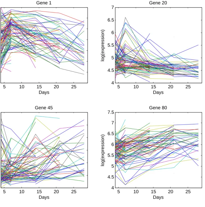
bi-nary outcome (complicated vs. uncomplicated recovery), survival out-come (time to recovery), and no outout-come. . . 56 3.2 Gene expression trajectories of representative genes from different

(10)

List of Tables

1.1 Parameter estimates resulting from simulation for the model with and without outcome with N=80 patients, J=50 genes, and 100 replications with 5000 iterations each. . . 15 1.2 Results of Glue Grant trauma data analysis with and without a

continu-ous outcome (maximum MOF score). . . 21 2.1 Results of Glue Grant trauma data analysis with a binary outcome

(com-plicated vs. uncom(com-plicated recovery) and survival outcome (time to re-covery). . . 37 3.1 Glue Grant array count on various days following injury. . . 54 3.2 Results of longitudinal Glue Grant trauma data analysis with a binary

outcome (complicated vs. uncomplicated recovery) and survival out-come (time to recovery). . . 57

(11)

Acknowledgments

I owe a great debt of gratitude to my advisors, Dianne Finkelstein and David Schoenfeld, for their guidance through the research process. I am immensely thank-ful for their invaluable expertise and unwavering faith in me. Working with them has truly been a wonderful learning experience. I would also like to thank Rebecca Beten-sky for providing me with many insightful suggestions and ideas.

I will forever be grateful to my friends who have supported me every step of the way. I especially want to thank Leesa Lin for showing me the meaning of true friend-ship and Shannon Stock for bringing so much sunshine into my life. I will also always cherish the joyful memories and friendships that HSPH Dance Club has given me over the years.

I would like to thank all my friends in the department, including Kate Jie Hu, Sabrina Khan, Rui Wang, Alisa Stephens, Anna Snavely, Lei Quanhong, Sharon Lutz, Miguel Marino, Mariel Finucane, Betsy Ogburn, Bonnie Zhang, Jeanne Jiang, Huan Huang, Zeynep Coban, Rui Zhao, Keith Betts, Roland Matsouaka, Alfa Yansane, and Alane Izu.

I would also like to thank my friends from home, including Arpi Shaverdian, Shirley Chou, Leigh Momii, Cheryl Hou, and Michelle Chan.

Most of all, I am grateful to my mom, dad, and sister for their unconditional love and support. Thank you Sherrie for being my best friend and always making me laugh. No matter where I am or what I am doing, my family has always given me a place to call home.

(12)

A Bayesian Approach to Informatively Clustering

Microarray Data

Jessie J. Hsu, Dianne M. Finkelstein, and David A. Schoenfeld

Department of Biostatistics, Harvard School of Public Health

(13)

1.1

Introduction

In the past decade, new technologies for high-throughput genomics and proteomics have developed with the potential of revolutionizing medicine. Gene expression mi-croarrays are one such technology that measure the levels of RNA expression in a cell. These expression levels are constantly changing, producing a rich influx of informa-tion. Due to the wealth of potential knowledge encoded in the human genome that is captured in microarray experiments, there is substantial interest in identifying differ-ential gene expression patterns and relating gene activity to phenotypic information.

Our goal is to reduce a microarray dataset into clusters of genes that are biologically meaningful and to use those clusters to predict patient outcome. We would like to find clusters of genes that are both correlated with each other as well as associated with pa-tient outcome, and we hypothesize that using outcome information to drive the pattern discovery can potentially result in gene clusters that are more coherent and biologically meaningful. We are motivated by the Inflammation and Host Response to Injury re-search program, also known as the Glue Grant (http://www.gluegrant.org). The Glue Grant is a large-scale interdisciplinary study of inflammation following severe trauma or burn injury. The immune system reacts to injury by activating the inflammation response in an attempt to prevent further damage to the body, and presumably the chain of events that takes place as the body tries to stabilize and recover is reflected in differential gene expression. The general aims of the Glue Grant are to uncover the biological reasons why patients have such varying responses following their injury, to understand the genomic and proteomic markers that predict clinical outcomes, and to determine the relationship between changes in gene expression and clinical features. For this paper, we focus on the association between patterns in differential gene ex-pression and metabolic recovery in patients with severe trauma.

Many methods have been developed for relating gene expression to clinical outcomes, most of which involve reducing the dimensionality of the gene expression data. One

(14)

way to go about this is to identify a subset of genes that are predictive markers of out-come. The simplest method for subset selection is univariate variable selection, where each gene is individually tested for significance and the top ranked ones are included in a multivariate model. Stepwise selection procedures achieve the same end but can be unstable for high-dimensional datasets. Increased stability and reduced prediction error can be obtained by penalized regression methods which operate by imposing a constraint on the parameters, leading to coefficient shrinkage (Tibshirani, 1996). In particular, lasso simultaneously obtains parameter estimates and achieves variable se-lection because the absolute value constraint causes some coefficients to be estimated at exactly zero. Dimension reduction can also be accomplished by principal components regression (Hastie et al., 2001a). This is an unsupervised procedure that reduces the gene expression values down to their principal components and incorporates the first few components that explain the majority of the predictor variation into a regression model. A supervised version of this approach is partial least squares regression (PLSR) (Parket al., 2002). Here, both the predictors and outcome are decomposed such that the latent vectors used in the decomposition maximize their covariance. Given that our goal of using outcome information to drive the data reduction is partially addressed by PLSR, we will use it for comparison to our method.

Clustering is another widely used form of microarray dimension reduction that is based on the assumption that groups of genes are more similar to each other than oth-ers for reasons such as related functionality, shared biological pathways, or a similar effect on outcome. One approach, though computationally burdensome, is to perform a stochastic search across the entire space of possible partitions and select the true clustering to be the one with the highest likelihood. Another approach is to cluster the genes across patient samples via a technique such as K-means and then to use the cluster expression averages in a regression model (Eisenet al., 1998). K-means cluster-ing is a classic clustercluster-ing algorithm that finds the partition of K sets that minimizes the distance of each observation to its center, where each cluster center is the mean of the

(15)

observations in that cluster (Hartigan, 1975). Achieving the optimal clustering using K-means with a Euclidean distance metric is equivalent to maximizing the likelihood that corresponds to modeling gene expression as a normally distributed cluster spe-cific fixed effect. The maximum likelihood occurs when each gene is assigned to its nearest cluster center such that the within cluster sum of squares is minimized. This approach operates under the assumption that all the genes to be clustered are inde-pendent. This is appropriate for clustering independent individuals but is flawed for clustering features that have a correlation structure. Rather, it is more reasonable to state that genes in the same cluster are correlated while genes across different clusters are independent. Furthermore, K-means assumes that there is only one correct cluster-ing pattern and does not provide a measure of uncertainty associated with the cluster assignments.

A related formulation of the clustering problem is the normal mixture model, where each observation is viewed as arising from a mixture of distributions. Fraley and Raftery (1998) and Ghosh and Chinnaiyan (2002) discussed model-based clustering where the gene expression data is modeled as a normal mixture and clusters are de-termined by the Expectation-Maximization (EM) algorithm. A Bayesian approach can also be used to fit the mixture model (Voglet al., 2005). In these approaches, the prob-ability distribution of each gene is modeled as the sum of K weighted underlying dis-tributions, each representing the distribution of a gene conditional on membership in each cluster. The entire data likelihood is then a product across all the genes. Once again, this approach fails to specify any sort of correlation between genes in the same cluster. These types of mixture models are valid for clustering patients, but do not reasonably extend to the setting of clustering features measured on each patient.

The statistically sound approach for model-based clustering is to include a random effect such that highly correlated genes fall in the same cluster. Nget al.(2006) imple-mented an EM algorithm to fit the random effects model for clustering. Alternatively, the Bayesian paradigm provides a unified framework for fitting complex hierarchical

(16)

models. For example, Boothet al. (2008) proposed a random effects clustering model and performed a stochastic search for clusters using the posterior distribution of the unknown partition as the objective function. Tadesseet al.(2005) presented a Markov chain Monte Carlo (MCMC) sampling scheme for simultaneously selecting discrimi-nating genes and clustering patients. The advantage of the Bayesian approach is that it accounts for uncertainty in all of the parameters, including variation about cluster membership. It can incorporate prior information and naturally allows outcome to drive the clustering of the genes when fitting the joint model.

The notion of outcome-informed clustering has been studied less extensively. Hastie et al.(2001b) touched upon the idea of informative clustering in his proposal of a su-pervised approach called ‘tree-harvesting’ where clusters of genes are explored in a stepwise fashion and related to outcome using the intermediate results of hierarchical clustering. Dettling and B ¨uhlmann (2002) discussed a strategy that directly incorpo-rates the response variable into the clustering process by using a rank-based test statis-tic for finding groups of genes that discriminate a categorical response. Ideally, one would like to simultaneously find clusters and model the outcome such that each part is influenced by the other.

In this chapter, we propose a joint model for simultaneously clustering correlated gene expression data and predicting a continuous patient outcome. We use a random effects model for describing gene expression cluster membership and relate the latent cluster effects to a continuous patient outcome via a linear model. We develop a MCMC clus-tering algorithm for model fitting and parameter inference based on a marginalized likelihood. By simultaneously modeling patient outcome with gene expression and developing a clustering algorithm that makes use of clinical data, we will generate clusters that are more useful for describing the clinical course of injury.

Our methodology is described in Section 1.2. The results of simulation studies are pre-sented in Section 1.3, and an analysis of the Glue Grant data is prepre-sented in Section 1.4.

(17)

We conclude with a discussion in Section 1.5.

1.2

Methods

1.2.1

Model Specification

We propose a joint model for clustering correlated gene expression data that is driven by a continuous patient outcome. Consider representing the microarray dataset as a

N×Jmatrix consisting of gene expression values forJgenes measured onNpatients. Let Yij be the gene expression value for patient i and gene j belonging in cluster k. Conditional on membership of genej in thekth _{cluster, the random effects model for} describing gene expression is

Yij =cik(j)+ij (1.1)

where i = 1, ..., N, j = 1, . . . , J, andk = 1, . . . , K. Here, cik(j) are patient-cluster spe-cific random effects that represent the cluster centers and induce correlation between genes in the same cluster. We assumecik(j) ∼ N(0, τ2)after the data have been log-transformed and centered to have mean zero. We also assume that cik and cik0 are

independent fork 6=k0. Thus, for a given patient, the covariance between genes in the same cluster isτ2 _{while genes in different clusters and across different patients remain} independent. Theij are measurement errors, assumed to be distributedN(0, σ2). To link the gene clusters to patient outcome, we specify a linear relationship between the clusters andZi, a continuous outcome for patienti,

Zi = K X

k=1

βkcik(j)+ξi. (1.2)

The cluster effects relate gene expression and patient outcome to each other by acting as covariates in the regression model. Theβk are the respective regression coefficients for each cluster, and the error terms are assumed to beξi ∼N(0, γ2).

(18)

φjk is an indicator denoting membership of gene j in cluster k. Additionally, letω =

(ω1, . . . , ωK)be the cluster weights withωk > 0for allk and P

k

ωk = 1. These weights represent the probability of belonging in each cluster.

1.2.2

Joint Likelihood

We will work with the marginal likelihood where the random effectscare integrated out:

f(Y, Z|σ, τ, β, γ, φ, ω) =

Z

f(Y, Z|c, σ, τ, β, γ, φ, ω)f(c|τ)dc. (1.3)

This is for ease of computation, since the random effects are nuisance parameters and our model fitting procedure is facilitated by not having to estimate all of them. A closed form expression for (1.3) is readily achieved, as described next, because the random effects are normally distributed.

Let Xi = (Yi, Zi), the vector of observations associated with patient i, where Yi =

(Yi1, ..., YiJ). LetΘdenote the set of parameters{σ, τ, β, γ, φ, ω}. The resulting complete data likelihood for(Y, Z)is given by a multivariate normal distribution,

f(Y, Z|Θ) = N Y i=1 exp{−1 2X 0 iΣ −1_X i} (2π)(J+1)/2_|_Σ_|1/2 .

The covariance matrixΣis a symmetric(J+ 1)×(J+ 1)matrix that is block diagonal in all but the last row and column. It is represented by

Σu,v =σ2I(u=v) +τ2 K P k=1 I(u, v ∈Sk) Σu,J+1 =τ2 K P k=1 I(u∈Sk)βk ΣJ+1,J+1 =τ2 K P k=1 β_k2+γ2 (1.4)

where the subscripts index the matrix elements. Here, u = (1, . . . , J), v = (1, . . . , J), andSk denotes thekthcluster set.

(19)

A closed form expression exists for both the inverse and determinant ofΣ. Therefore, the expression for the multivariate normal distribution simplifies substantially, speed-ing up computation of the Metropolis-Hastspeed-ings algorithm.

1.2.3

Prior Distributions for Model Parameters

We specify a non-informative prior distribution for every parameter. The prior for σ

is set to be uniform on a wide range. We also specify a uniform prior on a wide range for the hierarchical parameter τ, as recommended by Gelman (2006). The standard non-informative prior is used for the regression parameters(β, γ2₎_∝_1/_γ2_.

Non-informative conjugate priors are specified for ω and φ. A symmetric Dirichlet prior is set for the weights, P(ω1, . . . , ωK) ∝ Dirichlet(α, . . . , α). Larger values of α reflect the presence of more clusters, while smaller values of α reflect fewer clusters. Lastly, the cluster membership variableφhas a multinomial prior that depends on the weights,P(φjk = 1) =ωk.

1.2.4

MCMC Clustering Algorithm

We fit the model by implementing a MCMC algorithm that consecutively samples ev-ery parameter until a sufficient representation of the posterior distribution is achieved. The MCMC sampling procedure consists of repeating the following six steps until con-vergence:

1. Sampleσ2_.

2. Sampleτ2_.

3. Sampleφ.

(20)

5. Sampleβ.

6. Sampleγ2_.

Gibbs sampling is used for sampling the parameters that have an available full condi-tional posterior distribution. The set of samples obtained through multiple iterations estimates the posterior distribution of that parameter. When the full conditional dis-tribution cannot be directly sampled from, we use the Metropolis-Hastings algorithm. Candidate values are drawn from a proposal distribution and accepted with probabil-ity proportional to the ratio of the posterior densprobabil-ity evaluated at the current value to the posterior density evaluated at the new value. That is, samples are accepted with probability

min(1,P(θ

∗_|_{Y, Z}₎_/Q₍_θ∗_|_θ0₎

P(θ0_|_{Y, Z}₎_/Q₍_θ0_|_θ∗₎)

whereQis the proposal density,P is the posterior likelihood,θ0 is the current parame-ter value, andθ∗ is the candidate parameter value.

Update of variance parameters

The Metropolis-Hastings algorithm is used to sample σ2, τ2, and γ2. We use an in-verse gamma proposal distribution with shape parameter s and scale parameters/θ. These tuning parameters are determined experimentally during initial runs to accept proposed samples at the recommended rate of40%−45%(Gelmanet al., 2004).

Update of cluster membership and weights

Cluster membership φ is sampled from a multinomial distribution with probabilities proportional to the likelihood given the current parameter values. For every gene, we calculate the likelihood of belonging in each of the K clusters. The value of the likelihood weighted by the current value ofωthen becomes the updated multinomial

(21)

sampling probabilities. We sample directly from the full conditional distribution, given by f(φj|Y, Z, σ, τ, β, γ, ω)∝ K Y k=1 (f(Y, Z|σ, τ, β, γ, ω)∗ωk)φjk.

After sampling the cluster memberships of all the genes,ωis sampled via a Gibbs step. The full conditional distribution ofω is Dirichlet(α+n1, ..., α+nK), where nk is the current number of genes in thekth_cluster.

Update of regression coefficients

The regression coefficients β are sampled as a block by a Metropolis-Hastings algo-rithm. We specify a multivariate normal proposal distribution with an independent mean that is continuously updated whenever φj is updated in step 3. When a gene is assigned to a different cluster, the average of the coefficients of the original cluster and the new cluster become the new coefficients for the respective clusters. The re-sulting value after updating all the φj is then used as the proposal mean. As for the proposal covariance, we found through initial experimental runs that a covariance of 0.2*I, where I is the identity matrix, produces an acceptance rate near the recommended rate of20%−25%.

1.2.5

Model Without Outcome

The random effects clustering model in (1.1) can stand alone as a special case of the full joint model. In this simple case, f(Y|σ, τ, φ, ω) is a multivariate normal density with covariance matrix equal to (1.4) with the last row and column removed. Simplifying the likelihood expression leads to

f(Y|σ, τ, φ, ω) = exp{−1 2 N P i=1 [σ−2 K P k=1 (P j∈Sk (Y_ij2)− τ2 σ2_+n kτ2( P j∈Sk Yij)2)]} [(2π)J₍_σ2₎J−K QK k=1 (σ2₊_n kτ2)]N/2 .

(22)

Estimates of the unknown parameters are obtained by Metropolis-Hastings sampling in the same manner as previously described. We found that the random effects model does in fact cluster genes differently from the fixed effects model. To illustrate ana-lytically, we make the simplifying assumption that there is an equal number of genes in every cluster and derive an expression for the log-likelihood that has the variance components profiled out. As expected, the profile log-likelihood for the fixed effects model is maximized when each gene is as close as possible to its cluster center,

L∝X i X k X j∈Sk (Yij −Yik)2.

Interestingly, for the random effects model,

L∝X i X k X j∈Sk (Yij −Yik)2∗n X i X k (Yik)2.

This result implies that genes are clustered in a way that not only minimizes the dis-tance to the cluster centers, but also shrinks the cluster means towards zero.

1.2.6

Determining the Number of Clusters

Though the true number of non-empty clusters is unknown, it does not need to be sampled separately in our algorithm because an estimate of K is obtained at every iteration as an immediate result from the samples of cluster membership. Recall that

P(φjk = 1)is proportional to the weighted likelihood of belonging in clusterk. These multinomial probabilities are always non-zero becauseωkis positive for allkregardless of cluster size. Due to the probabilistic nature of the allocation, there is always a chance that a cluster will end up with no genes, or that an empty cluster will become filled at any given iteration. Therefore, the only value that needs to be specified in advance is Kmax, the maximum number of clusters. Kmax can also be thought of as the total number of both empty and non-empty clusters, where0≤K ≤Kmax.

(23)

1.2.7

Posterior Inference

Posterior Distributions

The MCMC algorithm outputs samples from the posterior distribution of each of the parameters and can be characterized by its posterior mean and posterior credible in-terval. We make an exception for φ and instead summarize its posterior distribution by the concordance between every pair of genes, where concordance is measured as the percentage of iterations that a pair of genes falls into the same cluster. Displaying cluster membership as a heat map allows the relationship between genes to be cap-tured and circumvents the issue of label switching which can cause the appearance of non-identifiability. The other cluster-dependent parameters, β and ω, can also ap-pear non-identifiable as a consequence of label switching. A remedy is to index these parameters by genes rather than by clusters.

Prediction

Given microarray data for a new patient, the predictive density of that patient’s out-come can be obtained. SinceZi and Yi are both normally distributed, f(Zi|Yi)is also normally distributed. Its expected value and variance are given by

E(Zi|Yi) = τ2 K X k=1 βk σ2₊_n kτ2 (X j∈Sk Yij) V ar(Zi|Yi) =τ2σ2 K X k=1 β2 k σ2₊_n kτ2 +γ2.

This distribution allows us to estimate the expected value of a future patient’s outcome based on their expression values.

(24)

1.3

Simulations

Simulations were conducted to evaluate the performance of our algorithm and to study the effect of outcome inclusion and different parameter values on the resulting clusters. In the first simulation study, we generated 100 datasets under the model without out-come and 100 datasets under the model with outout-come. Each set of data consisted of 80 patients and 50 genes arising from 5 clusters. We considered various values ofτ2 to assess the ability of our method to detect the correct cluster structure when cluster variation is low and when cluster variation is high compared to the variation in the residual error. This ratio, τ2_/σ2_{, is what we will refer to as the variance ratio. The} re-maining parameter values were set toσ = 1, γ = 1, β1 = −3, β2 = −1, β3 = 2, β4 = 3, andβ5 = 5. We setα = 1for the Dirichlet prior andKmax = 10. For every dataset, we ran 10,000 iterations and discarded 5,000 as burn-in.

A visual representation of the simulation results is presented in Figure 1.1. Cluster membership is depicted as a heat map that shows the proportion of iterations that every pair of genes is assigned to the same cluster. In the event of label switching, summarizing the output as a heat map aids in visualizing the groups, but even in the absence of label switching, the heat map has the advantage of providing informa-tion about the uncertainty surrounding the allocainforma-tions. We do not assume thatφ is a fixed value, but rather a parameter with a distribution where some groupings are more likely than others. Heat maps for the models with and without outcome are shown for

τ2_/σ2 _{= 4} _and _τ2_/σ2 _{= 0}_.₂_{. The genes are listed along both axes in the same order,} grouped together by their true cluster membership. Concordance is represented as a gradient from white (0%) to red (100%) with 16 discrete shades of color.

As depicted in the heat maps in Figure 1.1, the clustering is very clear when the vari-ance ratio is large regardless if outcome information is used. On the other hand, we observe a weak signal when the variance ratio is small. However, the clusters become

(25)

10 20 30 40 50 10 20 30 40 50 ττ2 _σσ2₌₌ 4 with outcome Genes Genes 10 20 30 40 50 10 20 30 40 50 ττ2 _σσ2₌₌ 4 without outcome Genes Genes 10 20 30 40 50 10 20 30 40 50 ττ2 _σσ2₌₌ 0.2 with outcome Genes Genes 10 20 30 40 50 10 20 30 40 50 ττ2 _σσ2₌₌ 0.2 without outcome Genes Genes

Figure 1.1: Cluster heat maps for simulated data. Concordance varies from 0% (white) to 100% (red).

(26)

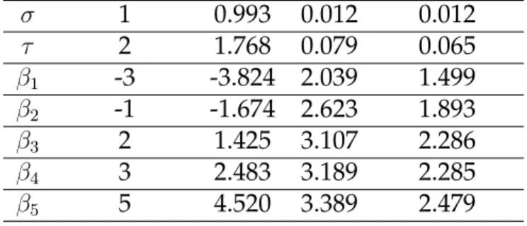
Table 1.1: Parameter estimates resulting from simulation for the model with and with-out with-outcome with N=80 patients, J=50 genes, and 100 replications with 5000 iterations each.

True value Mean SE Mean of SE

With outcome σ 1 0.993 0.012 0.012 τ 2 1.768 0.079 0.065 β1 -3 -3.824 2.039 1.499 β2 -1 -1.674 2.623 1.893 β3 2 1.425 3.107 2.286 β4 3 2.483 3.189 2.285 β5 5 4.520 3.389 2.479 Without outcome σ 1 0.993 0.012 0.012 τ 2 1.780 0.079 0.065

Table 1.1 displays posterior summary statistics of the parameters that result from the simulation when the variance ratio is large. We see that they are all well estimated by the MCMC algorithm. Note that estimation of the βk only makes sense when the algorithm has converged to a stable pattern and is conditional onK = 5in the current case. When there is substantial uncertainty in the clustering output, it is not possible to report averaged values forβk because there are different sets of βk associated with different values ofK. However, when the majority of the genes cluster in the same way across iterations, we can restrict ourselves to those iterations that estimated 5 clusters and expect that the averages are reasonable estimates of the true value.

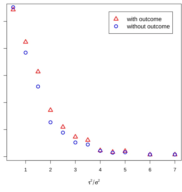
A second simulation study was conducted to understand the effect of the variance ratio on cluster uncertainty. Uncertainty is defined as the frequency of pairwise clus-tering inaccuracies as compared to the true cluster pattern. For this we considered a small dataset with 15 patients and 6 genes arising from 3 clusters with every two genes belonging to the same cluster. We variedτ2 _{to range from 0.5 to 7, while the other} pa-rameters were fixed atσ = 1, γ = 1, β1 =−2, β2 = 1,andβ3 = 3. For every case, 10,000

(27)

iterations were run with half discarded as burn-in. The model was fit both with and without outcome, and uncertainty was calculated for the range of variance ratios. The results are plotted in Figure 1.2. Given the described clustering pattern, the maximum amount of uncertainty that can be attained is 0.33. Asτ2_/σ2 _{increases, the uncertainty} decreases towards zero and we see that clustering with outcome consistently produces less uncertainty than clustering without outcome.

When the clustering signal is strong, that is whenτ2 _{is large, the clustering parameter} tends to converge quickly to the correct answer. Though this is advantageous, the drawback is that the clustering parameter does not mix as well as one would hope. This is because our algorithm only considers moves of one gene at a time, so the likelihood tends to not change enough to accept reallocations of a single gene. Nevertheless, there is no apparent need to over-explore the partition space when there is a strong signal because we still obtain convergence to the right clustering pattern. On the other hand, when the clustering signal is weak or nonexistent, mixing is irrelevant because the algorithm cannot reach convergence anyways due to a weak signal. It is in the case of a moderate signal that we would most want to see good mixing and hope that the frequency of genes clustering together is reflective of the probability of belonging in the same cluster. In the simulation setting, the lack of mixing in any given dataset is circumvented by averaging across all the simulated datasets. This is effectively the same as implementing several chains for every run and averaging across the chains, which is what we proceed to do in the Glue Grant data analysis.

1.4

Application

We applied our methodology to the Inflammation and Host Response to Injury trauma data, a rich dataset that contains information on numerous factors related to the biol-ogy of inflammation following severe traumatic injury. There are a total of 167 patients in the trauma dataset, each of whom has their blood leukocyte expression levels

(28)

mea-1 2 3 4 5 6 7 0.00 0.05 0.10 0.15 0.20 0.25 ττ2 _σσ2 Cluster Uncer tainty ● ● ● ● ● ● _● ● _● _● ● ● ● with outcome without outcome

Figure 1.2: Plot of cluster uncertainty with and without outcome for different variance ratios.

(29)

sured on an Affymetrix microarray chip consisting of 54,674 probe sets (which we will henceforth call ‘genes’). The full dataset consists of microarrays that have been taken at seven different time points following the patients’ injury, starting from immediately after the injury to up to 28 days later. For our analysis however, we restrict ourselves only to microarray data collected on day four from the 147 patients who are still in the intensive-care unit at that time.

The gene expression values have been pre-processed using dChip, log-transformed and centered prior to analysis. We use a subset of 87 genes for our cluster analysis. These genes were pre-selected by Glue Grant investigators to be those that had signif-icant differential expression with at least a two-fold difference between patients with a clinical outcome of complicated versus uncomplicated recovery. Our objective is to find clusters of genes that are associated with each other as well as associated with a relevant patient outcome. The outcome that we use in our analysis is maximum multi-ple organ failure (MOF), a continuous score that describes the severity of the patient’s multiple organ failure and is predictive of metabolic recovery. MOF is the cumula-tive sum of individual scores from the respiratory, renal, hepatic, cardiovascular, and hematologic components, each ranging in value from 0 to 4 for least to most severe. The resulting groups of genes can then be examined for their functional relationships and interdependent roles in the inflammation response pathway.

We ran ten MCMC chains, each starting from a different set of randomly chosen over-dispersed starting values. Non-informative priors were specified for all the parame-ters; hyper-parameters were chosen to beα = 1andKmax = 15. We evaluated mixing and convergence by assessing the trace plots and observed that convergence occurred fairly quickly. As mentioned previously, we ran multiple chains to simulate good mix-ing and averaged across all chains. Thus, for each of the MCMC chains, we ran 10,000 iterations with 5,000 discarded as burn-in.

(30)

20 40 60 80 With outcome Genes THBS1 FOLR3 PTGS2 PTGS2 HLA−DQB1 HLA−DQA1 HLA−DQB1 CEA CAM8 MMP8 MMP8 OLFM4 LCN2 LTF TCN1 CD24 CEA CAM6 CD24 IFI44 HERC5 EPSTI1 CMPK2 IFIT1 IFI44L RSAD2 RSAD2 IFIT3 IFIT2 IFIT2 IFIT5 IFIT5 IFIT3 MX1 IFI6 XAF1 EPSTI1 ISG15 O AS3 IFI44 XAF1 XAF1 O AS2 O AS1 HLA−DRA HLA−DP A1 HLA−DRA HLA−DRB1 HLA−DRB1 HLA−DRB1 HLA−DPB1 PMAIP1 HLA−DMB HLA−DMA HLA−DRB1 TGFBI HLA−DP A1 CD74 GNL Y GNL Y LOC100127983 CDK5RAP2 CDK5RAP2 LOC399972 NAIP SLC26A8 LRG1 A TP6V1C1 IL1R1 GALNT14 A GFG1 SIP A1L2 PDGFC GRB10 NSUN7 PCOLCE2 TDRD9 ANKRD55 MIA T HGF D A CH1 VNN1 VNN1 IL1R2 IL1R2 OLAH OLAH OLAH 20 40 60 80 Without outcome Genes Genes THBS1 FOLR3 PTGS2 PTGS2 HLA−DQB1 HLA−DQA1 HLA−DQB1 CEA CAM8 MMP8 MMP8 OLFM4 LCN2 LTF TCN1 CD24 CEA CAM6 CD24 IFI44 HERC5 EPSTI1 CMPK2 IFIT1 IFI44L RSAD2 RSAD2 IFIT3 IFIT2 IFIT2 IFIT5 IFIT5 IFIT3 MX1 IFI6 XAF1 EPSTI1 ISG15 O AS3 IFI44 XAF1 XAF1 O AS2 O AS1 HLA−DRA HLA−DP A1 HLA−DRA HLA−DRB1 HLA−DRB1 HLA−DRB1 HLA−DPB1 PMAIP1 HLA−DMB HLA−DMA HLA−DRB1 TGFBI HLA−DP A1 CD74 GNL Y GNL Y ENSG00000254288 LOC100127983 CDK5RAP2 CDK5RAP2 LOC399972 NAIP SLC26A8 LRG1 A TP6V1C1 IL1R1 GALNT14 A GFG1 SIP A1L2 PDGFC GRB10 NSUN7 PCOLCE2 TDRD9 ANKRD55 MIA T HGF D A CH1 VNN1 VNN1 IL1R2 IL1R2 OLAH OLAH OLAH e 1.3: Cluster heat maps for Glue Grant trauma data with and withou t a continuous outcome (maximum MOF e). Concor dance varies fr om 0% (white) to 100% (r ed).

(31)

patient outcome is shown in Figure 1.3. The genes are listed along both axes in the same order for both plots. When the model is fit with outcome, the genes labeled 1-58 fall into seven distinct clusters the majority of the time upon convergence. These seven clusters are clearly distinguished by the red boxes along the diagonal starting from the bottom-left with the exception of some orange overlap between genes labeled 42 to 58 on the plot. It appears that about20%of the time, genes 57 and 58 form their own cluster of size two, while the remainder of the time they are part of the larger cluster. On the other hand, several breakdown combinations are observed for genes 59-87. They do not group into clear partitions, implying that several partitions have similar posterior probabilities.

When we fit the model without outcome, we obtain a heat map that appears compa-rable though there is more pronounced uncertainty. The general partition structure remains the same, but now there is more orange and yellow in some groups because the posterior pairwise probabilities are not as high. There are various subsets of genes that form their own clusters on occasion. The only genes for which there is actually less uncertainty are genes 85-87, as they now exclusively cluster together.

In both cases, clusters consisting of only one gene are allowed. Normally we may not wish to have singletons for a dataset that has thousands of genes, but since this is a fairly small subset of genes that was pre-selected to be important, we do not want to be too strict in forcing singletons into larger sized clusters.

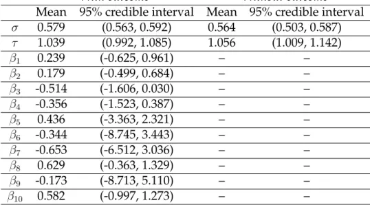
A summary of the output is shown in Table 1.2. The mean of the variance ratio is 3.22 for the case with outcome and 3.51 for the case without outcome. The uncertainty surrounding cluster membership is minimal because the estimated variance ratio is relatively large. The coefficient estimates are conditional onK = 10, where the clusters are of size 1, 1, 2, 3, 10, 24, 17, 1, 25, and 3 (from left to right in Figure 1.3). Only those iterations for which the genes in each respective cluster exclusively group together are used in calculating the coefficient estimate for that cluster.

(32)

Table 1.2: Results of Glue Grant trauma data analysis with and without a continuous outcome (maximum MOF score).

With outcome Without outcome

Mean 95% credible interval Mean 95% credible interval

σ 0.579 (0.563, 0.592) 0.564 (0.503, 0.587) τ 1.039 (0.992, 1.085) 1.056 (1.009, 1.142) β1 0.239 (-0.625, 0.961) – – β2 0.179 (-0.499, 0.684) – – β3 -0.514 (-1.606, 0.030) – – β4 -0.356 (-1.523, 0.387) – – β5 0.436 (-3.363, 2.321) – – β6 -0.344 (-8.745, 3.443) – – β7 -0.653 (-6.512, 3.036) – – β8 0.629 (-0.363, 1.329) – – β9 -0.173 (-8.713, 5.110) – – β10 0.582 (-0.997, 1.273) – –

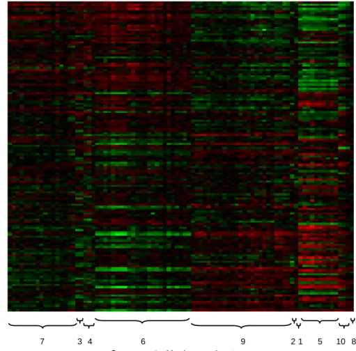
Figure 1.4 displays a heat map of the gene expression data that has been sorted ac-cording to the clustering results. Every row is a patient, where the patients are sorted by increasing MOF, and every column is a gene, where the genes are sorted by the mean of the regression coefficient of their respective clusters. Gene expression val-ues have been centered at zero in both directions; red represents under-expression and green represents over-expression. The cluster groupings are denoted by the brackets along the bottom of the figure. As expected, different values of MOF are associated with different gene expression patterns, and genes in the same cluster have similar ex-pression patterns, Furthermore, clusters with a positive coefficient have an opposite pattern from clusters with a negative coefficient. Cluster nine is the one exception. Even though the mean ofβ9 is negative yet the pattern implies the opposite, its value is very close to zero and suffers from high variability. Substantial cluster uncertainty surrounding cluster nine accounts for its high coefficient variability and expected in-stability.

(33)

7 3 4 6 9 2 1 5 10 8

Figure 1.4: Heat map of sorted gene expression data. Red represents under-expression and green represents over-expression. The numbers correspond to the cluster labels in Table 1.2.

(34)

squares regression is 9.61 conditional on K=10. In addition to having a lower MSE, our method fulfills the additional purpose of providing interpretable gene clusters.

1.5

Discussion

We have proposed Bayesian methodology for the informative clustering of genes. Our model accounts for correlation between genes in the same cluster and jointly relates the gene expression values to a continuous patient outcome such that this additional information helps drive the clustering of the genes.

It would be worthwhile to consider relaxing some of the assumptions of our model. For example, a heterogeneous covariance structure where a different τk is specified for every cluster would allow for more flexibility. A non-linear relationship between the clusters and outcome could also be modeled. We mentioned some solutions to deal with the mixing problem, but the best way to handle this issue would be to incorporate global moves such as splitting or combining clusters. Though this would allow the partition space to be explored more fully, it would add extra computational complexity.

Our model can be extended to accommodate categorical outcomes using a probit or logistic model, or time to event outcomes using semi-parametric models. Additionally, the model can be extended to the longitudinal microarray setting where it is assumed that groups of genes cluster together in their patterns over time.

(35)

Latent Variable Methods for Clustering Genes Using

Binary and Failure Time Outcome Data

Jessie J. Hsu, Dianne M. Finkelstein, and David A. Schoenfeld

Department of Biostatistics, Harvard School of Public Health

(36)

2.1

Introduction

The relationship between microarray data and binary patient outcomes is generally framed as a classification problem (Ring and Ross, 2002; Quackenbush, 2006). Gene expression data can be highly predictive of clinical outcomes such as disease type, as demonstrated in Golub et al. (1999). Microarrays can also be used to distinguish be-tween different diseases. For example, Dudoitet al.(2002) compares nearest-neighbor classifiers, linear discriminant analysis, and classification trees for discriminating ma-lignant versus normal tissue based on gene expression data in cancer patients. On the other hand, modeling the relationship between gene expression and binary outcomes using logistic regression can also lead to models that are highly descriptive of outcome.

The association between microarray data and survival outcomes can be studied in a similar manner. Typically, the objective of these studies is to determine the hazard of experiencing the event that is associated with the observed expression measurements. Jung et al. (2005) and Gui and Li (2005) developed methods for identifying a subset of genes that are biologically important and predictive markers of survival. In an ap-proach suggested by Bair and Tibshirani (2004), each gene is given a Cox score based on the proportional hazards partial likelihood and the top ranked ones are included in a multivariate Cox model. A comprehensive overview of predicting patient survival from microarray data is presented in Bøvelstadet al.(2007) and Wieringenet al.(2009).

Due to the high-dimensionality of microarray experiments, dimension reduction is of-ten a necessary step in data analysis. Common methods for dimension reduction in-clude principal component analysis and partial least squares, both of which reduce the expression values to fewer dimensions based on correlation. If outcome information is available, a supervised approach is generally preferred. Though these methods have been extended to both binary and survival settings (Nguyen and Rocke, 2002; Park et al., 2002), the drawback is they do not give interpretable components.

(37)

We use clustering as a form of dimension reduction and as a way to gain insight into underlying gene expression patterns. A standard cluster analysis involves a two-step process where clustering is performed by a method such asK-means and the cluster averages are used as covariates to model outcome. However, ideally we would like to find clusters and simultaneously predict outcome such that each part is influenced by the other. To this end, the Bayesian approach for model fitting is a natural way to allow for outcome-driven clustering of gene expression data due to its iterative approach. Previous Bayesian contributions in the realm of clustering multivariate data include Booth et al. (2008) and Tadesse et al. (2005), both of whom use Markov chain Monte Carlo (MCMC) methods for clustering data. For our contribution, we seek to use pa-tient outcome to inform the discovery of gene clusters with the hope that the resulting clusters provide a more coherent depiction of the underlying biological mechanism.

We propose a joint model that relates clusters of gene expression measurements to bi-nary and event time outcomes. Our model for gene expression adds complexity to standard mixture models (McLachlanet al., 2002) by incorporating cluster and subject specific random effects. These random effects account for correlation between genes in the same cluster and allow us to extend the mixture-model construction to the setting where non-independent patient features are being clustered. For a binary outcome, the probability of experiencing the event is related to the clusters via the introduction of la-tent continuous variables into the model. The lala-tent variables are then linearly related to the cluster random effects which transforms the model into the standard linear re-gression formulation. Conditional on the continuous latent response, the methodology for estimating the posterior distribution of the parameters is equivalent to clustering using a continuous outcome as described in Chapter 1. Obtaining these latent parame-ters is readily achieved by adding an extra step into the MCMC sampling scheme (Al-bert and Chib, 1993). An example of this type of Bayesian latent variable approach is described in Shaet al.(2004). In their paper, they augment a probit model with contin-uous latent variables to accommodate multinomial response variables for the purpose

(38)

of high-dimensional variable selection. We extend our binary model to accommodate survival data by treating time-to-recovery as a series of binary observations at a fixed number of discrete time points where the outcome at every time point is evaluated as a binary response. Again, we augment the data by assuming that the hazard of the event at any given time depends on a latent continuous variable. Then, a negative binomial model with a constant hazard of recovery is assumed for describing the amount of time that a patient is at risk.

Our method is applied to trauma data from the Inflammation and Host Response to Injury Program. Also known as the Glue Grant, this research project is an interdisci-plinary study of the biological changes that a patient goes through after experiencing severe trauma injury. The data consists of expression values measured on thousands of genes, as well as various clinical measurements and recovery endpoints for every pa-tient. Utilizing patient recovery to drive the process of clustering genes can potentially result in groups that more thoroughly capture the relationship between genes.

We proceed with a detailed description of the methodology in Section 2.2. The results of simulations are shown in Section 2.3. An analysis of microarray data from the Glue Grant is presented in Section 2.4, and we end with a discussion in Section 2.5.

2.2

Methods

2.2.1

Clustering Genes Using a Binary Outcome

For every subjecti, i = 1, . . . , N, we observe(Yi, Xi), whereYi is a vector of gene ex-pression values andXiis a single binary outcome. Our goal is to group the genes into several clusters based on similarities in their expression values and their association to the binary response. The genes should cluster in such a way that genes in the same cluster are highly correlated with each other, while genes in different clusters are

(39)

mu-to the response variable. In order mu-to obtain clusters with these properties, we will fit a joint model that relates the gene expression values to the binary outcome.

The first part of the joint model describes the observed gene expression data. We as-sume that the dependence among genes in the same cluster is induced by subject and cluster specific random effects. Thus, for genej belonging in clusterk, the model for gene expression is formulated as follows:

Yij =cik(j)+ij, cik(j) ∼N(0, τ2), ij ∼N(0, σ2) (2.1)

It can be shown that the presence of patient-cluster specific random effects in the model, represented bycik(j), results in a covariance ofτ2 between genes in the same cluster and a covariance of zero between genes in different clusters. We assume thatcik andcik0 are independent fork 6=k0. We also note that the reason that both the random

effects and the error terms have mean zero is because we assume the data have been centered at zero for every patient and gene prior to analysis.

Though the random effects provide information about the relationship between genes in different clusters, they provide no indication of the clustering pattern itself. It is therefore necessary to introduce additional parameters into the model to represent the unknown cluster membership. We use indicator variablesφjk to denote the member-ship of gene j in clusterk. We assume the vector of indicators associated with each gene has a multinomial distribution with probabilitiesωk,k = 1, . . . , K, whereωk >0

∀kand P k

ωk = 1. The entire clustering pattern can then be obtained directly from the matrix of cluster indicators.

The second part of the joint model describes the observed binary response. For every patienti,Xi is a Bernoulli(p) distributed random variable that equals one if the patient experienced the event. However, fitting a model that has a Bernoulli distributed ran-dom variable greatly increases the difficulty of implementing a MCMC because none of the posterior distributions are tractable. Therefore we facilitate the Bayesian model fitting procedure by introducing a normally distributed latent variableZi that will be

(40)

simulated by MCMC and assume that the probability associated withXi depends on

Zi. Known as the data augmentation approach (Tanner and Wong, 1987), Zi can be thought of as an unmeasured underlying process that directly determines the value of the observed binary responseXi. Augmenting the data to includeZirequires the spec-ification of a function that links the relationship betweenXi and Zi (Albert and Chib, 1993). In the context of data augmentation, the probit link is most commonly used:

P(Xi = 1) = Φ(Zi) (2.2)

where Φis the cumulative density function of the standard normal distribution. The dependence ofXionZiis straightforward; a smaller value ofZiimplies thatXiis more likely to be zero and a larger value ofZi implies thatXiis more likely to be one.

Up to this point, we have proposed separate models for the clusters of gene expres-sion data and for the binary outcome. The final layer of the model is to connect these two components together. The gene clusters are related to the binary outcome by a linear relationship between the cluster random effects and Zi, the continuous latent representation of the binary response:

Zi =µ+ K X

k=1

βkcik(j). (2.3)

This is essentially a linear regression model where the βk act as coefficients that de-scribe the effect of the cluster centers on the continuous latent outcome.

We noticed that whenβ was unconstrained, it tended to increase without bound. The reason this model may not converge is because we only observe Xi and have fewer degrees of freedom than provided by the normal model. We found that convergence occurs whenβis constrained to lie on the unit sphere such thatβTβ = 1. A convenient distribution for points on a sphere is the von Mises-Fisher distribution, which we detail in Section 2.2.2.

(41)

Prior Distributions

Non-informative prior distributions are specified for every parameter. The priors for the hierarchical standard deviation components σ and τ are uniform densities on a wide range. This is approximately equivalent to specifying an Inverse-χ2 _prior distri-bution onσ2 _and _τ2_{. For the vector of cluster probabilities} _ω_{, we specify a conjugate} symmetric Dirichlet(α, . . . , α)prior. Smaller values ofαreflect a prior belief that there should be fewer clusters and larger values drive the clustering towards more clusters. The cluster membership variable has a conjugate multinomial prior that depends on the weights,P(φjk = 1) =ωk. The intercept termµis given a non-informative uniform prior, and a von Mises-Fisher prior distribution with concentration parameterλ= 0is specified for the vectorβ. This parameter setting is non-informative and is equivalent to uniformity on a K-dimensional unit sphere.

2.2.2

MCMC Clustering Algorithm

The MCMC algorithm iterates between draws from the full conditional posterior distri-butionsf(Zi|Yi, Xi,Θ)for every patientiandf(Θ|Y, X, Z), whereΘdenotes the entire set of parameters{σ, τ, µ, β, φ, ω}. We exclude the random effectscfrom the parameter set because we will only be working with distributions that have the random effects integrated out so that they no longer appear in the likelihood. Carrying out this math-ematical detail greatly reduces the dimension of the parameter space and increases the stability of the algorithm.

(42)

con-ditional normal distribution with mean µZi|Yi,Θ = µ+τ 2 PK k=1 (βk/(σ2 +nkτ2))(P j∈Sk Yij) andσ2_Z i|Yi,Θ =τ 2_σ2 PK k=1 β_k2/(σ2+nkτ2).

Due to the difficulty of drawing Zi directly from (2.4), we utilize the acceptance-rejection algorithm for samplingZi. The acceptance-rejection algorithm for simulating random variables with density f(·) operates by finding a density g(·) from which it is easy simulate, along with a constantM such thatf(θ)/g(θ) ≤ M ∀θ. The algorithm proceeds by simulating valuesθ∗fromf(·)and accepting these values with probability

f(θ∗)/(M g(θ∗)). As a result, the elements in the set of values that are accepted will be random variables fromf(·).

In our case,f(·)is the expression in (2.4). If we letg(·) =φ(µZi|Yi,Θ, σ

2

Zi|Yi,Θ), thenM = 1

is an upper bound. SinceZ1, . . . , ZN are independent random variables, the steps in the algorithm are as follows:

1. GenerateZ_i∗ ∼φ(µZi|Yi,Θ, σ

2 Zi|Yi,Θ).

2. GenerateU ∼U nif orm(0,1).

3. IfU < [Φ(Zi)I(Xi = 1) + Φ(−Zi)I(Xi = 0)], then acceptZi∗; otherwise, rejectZ

∗

i.

Next, we need to sample fromf(Θ|Y, X, Z). Conditional on Z andY, it is not neces-sary to also condition on X because X gives no additional information given Z. To simulate any single parameterθfrom the setΘ, we write the full conditional posterior distribution forθ:

f(θ|Y, Z,Θ−θ)∝f(Y, Z|Θ)f(θ). (2.5)

Note that f(Y, Z|Θ) is a product across independent patients i, where f(Yi, Zi|Θ) is multivariate normal with mean(0, . . . ,0, µ)0and covarianceΣ, a symmetric(J+ 1)(J+

(43)

1)matrix that is block diagonal in all but the last row and column: Σu,v =σ2I(u=v) +τ2 K P k=1 I(u, v ∈Sk) Σu,J+1 =τ2 K P k=1 I(u∈Sk)βk ΣJ+1,J+1 =τ2 K P k=1 β2 k

where u = (1, . . . , J) and v = (1, . . . , J) index the matrix elements, and Sk denotes thekth cluster set. The expression for the multivariate normal distribution simplifies substantially because a closed form expression exists for both the inverse and the de-terminant ofΣ.

If the distribution represented by (2.5) is available in closed form for any given pa-rameter, basic Gibbs sampling is used and samples are drawn directly from the closed form distribution. If the full conditional posterior cannot be sampled from directly, we utilize the Metropolis-Hastings algorithm, where candidate values are drawn from a proposal distribution and accepted with probability proportional to the ratio of the posterior density evaluated at the current value to the posterior density evaluated at the new value. More explicitly, supposing thatθ0is the current parameter value andθ∗

is the candidate value, samples are accepted with probability

min(1,P(θ

∗_|_{Y, Z}₎_/Q₍_θ∗_|_θ0₎

P(θ0_|_{Y, Z}₎_/Q₍_θ0_|_θ∗₎)

whereQis the proposal density andP is the posterior likelihood.

Using the theory presented above, we continue describing the details of sampling each parameter inΘ. To simulate the variance parameters σ2 and τ2, the Metropolis-Hastings algorithm is used. We draw candidate values from an inverse gamma pro-posal distribution with shape parameters and scale parameters/θ. These tuning pa-rameters are determined experimentally during initial runs to accept proposed sam-ples at the recommended rate of40%−45%(Gelman, 2006).

The probabilities associated with belonging in each cluster are sampled via a Gibbs step. The full conditional distribution ofωis Dirichlet(α+n1, ..., α+nK), wherenkis the

(44)

number of genes in thekth_{cluster at the current iteration. We found that setting}_α _{= 1} provides a reasonable result. The cluster membership of each gene,φj, is sampled from a multinomial distribution with probabilities proportional to the weighted likelihood given the current parameter values. The clustering space is explored in a stochastic search where each gene is moved into every cluster and the likelihood of belonging in each of the K clusters is calculated. The value of the likelihood weighted by the current value ofωthen becomes the updated multinomial sampling probabilities.

The intercept term µ is sampled using Metropolis-Hastings. Candidate values are drawn from a normal proposal distribution with variance equal to one. The vector of coefficients,β, is obtained by Metropolis-Hastings sampling as well. As mentioned earlier, we constrainβto exist on theK-sphere such that the sum of squares equals one. The von Mises-Fisher (vMF) distribution for a unit vector of dimensionK has proba-bility density function f(x) = CK(λ)exp(λµTx)and is suitable for drawing candidate values with the desired constraint. Here, C is a constant, λ ≥ 0is the concentration parameter, andµis the mean direction. Following the steps described in Wood (1994) on how to sample from the vMF distribution, the result is aK-dimensional unit vector with modal direction(0, . . . ,0,1)T _{and concentration parameter} _λ_{. Applying QR} de-composition rotates the vector such that the modal direction is located at the proposed value ofβ.

2.2.3

Extension to Failure Time Outcome

Our proposed hierarchical model can be extended to time-to-event outcomes in a straightforward manner. We represent time-to-event as an indicator variable that is a function of time, Xi(t). If patient i experiences an event at time t, then Xi(t) = 1; otherwise if the patient has not yet had the event by time t, then Xi(t) = 0. Rather than observing a single binary endpoint, we now observe a vector of binary responses for every patient with one response at every time point. The responses are recorded at

(45)

fixed discrete time points until the patient is no longer in the risk set.

As in the case with a binary outcome, we utilize the data augmentation approach and introduce latent variablesZiinto the model, whereZiis normally distributed and mod-eled as shown in (2.3). LetLibe the number of times that patientiis evaluated for hav-ing the event. The hazard of the event at any particular timetl, l = 1, . . . , Li, depends onZias follows:

P(Xi(tl) = 1|Xi(tl−1) = 0) = Φ(Zi). (2.6)

For the purposes of illustrating our method, we assume that each patient has a constant underlying hazard of experiencing the event. However, this assumption can be relaxed to accommodate non-constant hazards with the inclusion of an additional parameter per time point. To model the amount of time that a patient is in the risk set, we assume a negative binomial distribution where the probability of success is simply the hazard of recovery as shown in (2.6). The probability of recovering at thelth _{time point then} becomesΦ(−Zi)l−1Φ(Zi).

The MCMC for fitting the survival model follows almost exactly the same steps as in the case of the binary outcome. The only difference occurs in step three of the acceptance-rejection algorithm because the full conditional posterior distribution ofZi is now a product across the time points:

Therefore we have the same function g(·) and the same constant M = 1, but ac-ceptance of Z_i∗ is now based on a comparison of the uniform random variable to

Li

Q l=1

(46)

2.3

Simulations

We conducted simulations to compare the effect of using an informative outcome against a non-informative outcome. For both, expression data was generated under the proposed model with fixed parameter values. In particular, we point out that we setτ = 0.5and σ = 1, which represents a fairly small amount of variability between the clusters compared to the residual variance. Non-related event outcomes were ob-tained by generating outcomes at random for every patient. We simulated 50 datasets for both informative and non-informative binary and failure time outcomes. Each set of data consisted of 80 patients and 50 genes arising from 5 clusters. For every dataset, we ran 5000 iterations and discarded 2000 as burn-in.

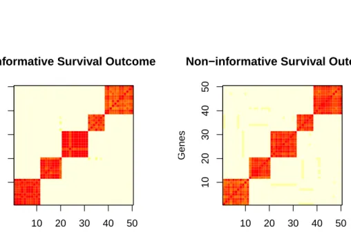
The cluster heat maps for the simulated data are presented in Figures 2.1 and 2.2. In both figures, having a non-informative outcome produces more uncertainty, where un-certainty is defined as the frequency of pairwise clustering inaccuracies as compared to the true cluster pattern. Given the described clustering pattern, random noise produces an uncertainty of 0.206. The uncertainties for an informative and non-informative bi-nary outcome are 0.042 and 0.068, respectively. The uncertainties for an informative and non-informative survival outcome are 0.043 and 0.047, respectively.

2.4

Application

The Glue Grant dataset contains information on numerous factors related to the bi-ology of inflammation following severe traumatic injury. Data on 147 subjects are included in the analysis, each of whom has their blood leukocyte expression levels measured on an Affymetrix microarray chip consisting of 54,674 probe sets (which we henceforth call ‘genes’). Arrays collected on day 4 following trauma will be used for the analysis, the reason being that allowing a few days to pass after the event will give

(47)

10 20 30 40 50 10 20 30 40 50

Informative Binary Outcome

Genes Genes 10 20 30 40 50 10 20 30 40 50

Non−informative Binary Outcome

Genes

Figure 2.1: Cluster heat maps for simulated data with a non-informative and informa-tive binary outcome.

10 20 30 40 50 10 20 30 40 50

Informative Survival Outcome

Genes Genes 10 20 30 40 50 10 20 30 40 50

Non−informative Survival Outcome

Genes

Figure 2.2: Cluster heat maps for simulated data with a non-informative and informa-tive survival outcome.

(48)

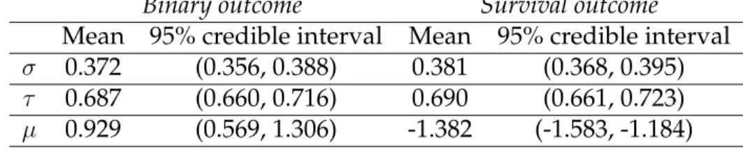
Table 2.1: Results of Glue Grant trauma data analysis with a binary outcome (compli-cated vs. uncompli(compli-cated recovery) and survival outcome (time to recovery).

Binary outcome Survival outcome

Mean 95% credible interval Mean 95% credible interval

σ 0.372 (0.356, 0.388) 0.381 (0.368, 0.395)

τ 0.687 (0.660, 0.716) 0.690 (0.661, 0.723)

µ 0.929 (0.569, 1.306) -1.382 (-1.583, -1.184)

The gene expression values have been pre-processed using dChip, log-transformed and centered prior to analysis. We use a subset of 87 genes for our cluster analysis that have been pre-selected by Glue investigators to be those that had significant differen-tial expression with at least a two-fold difference between patients with complicated versus uncomplicated recovery. Complicated recovery implies the patient had a time to recovery of more than 14 days, and patients with an uncomplicated status recovered in less than 14 days.

For both the binary and survival analyses, we ran eight chains with over-dispersed starting values. We ran 8000 iterations until convergence and discarded 2000 itera-tions as burn-in. The maximum number of clusters was set to be 15. For our method, we only need to specify the maximum number of clusters and not the exact number because our algorithm allows for empty clusters when the genes are tested for mem-bership against every cluster. However, since we only make single gene transitions when sampling cluster membership, there is a tendency to under-explore the parti-tion space. Therefore, several chains at different starting values were implemented and subsequently averaged for purposes of inference. Estimates of the parameters are shown in Table 2.1.

We define the event of interest to be complicated versus uncomplicated recovery class for the binary outcome. For the survival outcome, the response measurement is time to recovery from trauma. Patients are followed for 28 days, and time to recovery is calculated as the maximum time to cardiovascular, hematologic, hepatic, renal, or

(49)

res-piratory recovery. We assume that recovery can only occur once for every patient and that once recovery has occurred, the patient is no longer at risk. Recovery is the only absorbing state in the model; once a patient recovers, the patient is considered to have reached the end of the study. If patients do not recover during the course of the study or if they die prior to the last observed day, they are censored on day 28 and have an observed indicator vector that consists of all zeroes. Since only five of the 147 subjects died from their injuries, mortality was not considered an appropriately sensitive vari-able for informing distinct clusters. In addition to the five patients who died within the first 28 days, seven patients did not recover within the first 28 days. Both of these groups of patients are censored at 28 days since it is evident that none of these patients will recover by day 28.

A visual representation of clustering with and without outcome is presented in Fig-ure 2.3. Cluster membership is depicted as a heat map that shows the proportion of iterations that every pair of genes was assigned to the same cluster. The similarity, or concordance, between two genes is defined as the percentage of iterations that they are assigned to the same cluster. Concordance is depicted by a color gradient and ranges from 0% (white) to 100% (red). By representing the cluster results in a heat map, la-bel switching is accounted for and the allocation frequencies can be visualized clearly. In all three heat maps, the genes are aligned in the same order along both axes. The resulting partitions from using a binary outcome and from using a survival outcome appear similar to each other. Slightly different groups are found when clustering with-out with-outcome.

2.5

Discussion

In this chapter, we have developed methodology for using binary and failure time out-comes to inform the clustering of gene expression data. The intention is primarily for exploratory purposes, though the method can also be used for prediction. The clusters

(50)

20 40 60 80 20 40 60 80 Binar y Outcome Genes 20 40 60 80 20 40 60 80 Sur viv al Outcome Genes 20 40 60 80 20 40 60 80 No Outcome Genes e 2.3: Cluster heat maps for Glue Grant trauma data with a binary outcome (complicated vs. uncomplicated recov-survival outcome (time to recovery), and no outcome.

(51)

can act as prognostic markers in predicting recovery among trauma patients, making it possible to determine the posterior predictive probability that a future patient will experience the event. By augmenting the data with latent continuous variables, we are able to utilize the methods developed in Chapter 1. When applied to the Glue Grant data, we can determine the probability that a pair of genes are in the same cluster and identify