Remittances and the
Impact on Crime in
Mexico
Steve Brito
Ana Corbacho
René Osorio
Institutions for Development Sector
IDB-WP-514
IDB WORKING PAPER SERIES No.
Inter-American Development Bank
May 2014
Remittances and the Impact on
Crime in Mexico
Steve Brito
Ana Corbacho
René Osorio
2014
http://www.iadb.org
The opinions expressed in this publication are those of the authors and do not necessarily reflect the views of the Inter-American Development Bank, its Board of Directors, or the countries they
represent.
The unauthorized commercial use of Bank documents is prohibited and may be punishable under the Bank's policies and/or applicable laws.
Copyright © Inter-American Development Bank. This working paper may be reproduced for any non-commercial purpose. It may also be reproduced in any academic journal indexed by the American Economic Association's EconLit, with previous consent by the Inter-American Development Bank (IDB), provided that the IDB is credited and that the author(s) receive no income from the publication.
Contacts: Steve Brito, steveb@iadb.org; Ana Corbacho, acorbacho@imf.org; René Osorio, rosorio@iadb.org
Cataloging-in-Publication data provided by the Inter-American Development Bank
Felipe Herrera Library
Brito, Steve
Remittances and the impact on crime in Mexico / Steve Brito, Ana Corbacho, Rene Osorio. p. cm. — (IDB Working Paper Series ; 514)
Includes bibliographic references.
1. Emigrant remittances—Mexico. 2. Crime—Rates—Mexico. 3. Homicide—Rates—Mexico. I. Corbacho, Ana. II. Osorio, Rene. III. Inter-American Development Bank. Institutions for Development Sector. IV. Title. V. Series.
IDB-WP-514
Abstract*
This working paper studies the effect of remittances from the United States on crime rates in Mexico. The topic is examined using municipal-level data on the percent of household receiving remittances and homicides per 100,000 inhabitants. Remittances are found to be associated with a decrease in homicide rates. Every 1 percent increase in the number of households receiving remittances reduces the homicide rate by 0.05 percent. Other types of crimes are analyzed, revealing a reduction in street robbery of 0.19 percent for every 1 percent increase in households receiving remittances. This decrease is also observed using a state-level panel in another specification. The mechanisms of transmission could be related to an income effect or an incapacitation effect of remittances increasing education, opening job opportunities, and/or reducing the amount of time available to engage in criminal activities.
JEL Codes: J15, J22, O12, O15, O54
Keywords: Remittances; Migration; Crime; Homicides; Mexico
* This paper was prepared when Ana Corbacho was a sector economic advisor in the Institutions for Development Sector
at the Inter-American Development Bank (IDB). The authors wish to thank Christopher Woodruff and Maria Soledad Martinez for sharing their data on the distance along the rail network in 1920 and the distances along the rail network in 1998. Also, we thank Michele Coscia and Viridiana Rios for sharing their data on the location of drug cartel activities. We are grateful to Martin Ardanaz, Mario Cuevas, Guillermo Lagarda, Osmel Manzano, and Dean Yang for their valuable comments.
2
1.
Introduction
Mexico is a country with a long history of immigration to the United States. Mexican immigrants as a group are among the largest senders of remittances worldwide. Based on the amount sent from 2010 to 2012 (Figure 1), Mexico ranks third among remittance-receiving countries (5 percent of global remittances) and first in the Latin American and Caribbean (LAC) region (40 percent of the region). Mexicans are the also most numerous group of migrants in the world (nearly 12 million), mostly to the United States (World Bank, 2011). In 2010, Mexicans working in the United States sent back more than US$22 billion in remittances to family members, accounting for 2.1 percent of the Mexican GDP. Although remittances are a small part of the Mexican economy, they are the third source of foreign exchange after oil and manufacturing exports, and represent an amount greater than the international tourism receipts and foreign direct investment inflows. Moreover, for the poorest rural areas of Mexico, remittance transfers constitute 19.5 percent of their income, a percentage that is higher that transfers from government poverty reduction programs, such as the conditional cash transfer program Oportunidades (10.2 percent) and agricultural support programs, such as Procampo (3.8 percent) (World Bank, 2004).
Figure 1. Remittance in Mexico, Latin America and the Caribbean, and the World 2010–12 (in billions of dollars)
Source: Authors’ estimates based on World Bank data.
0 10 20 30 40 50 60 70 80
LAC India China Mexico Philippines South
America America Central Caribbean
3
The remittances that immigrants send back raise the incomes of recipients, enabling them to increase consumption and investment. Drawing on data from the Encuesta sobre Migración en la Frontera Norte de México (2005),1 Table 1 presents information on the main categories in which remittances are spent: 74 percent of them were used for consumption, 16 percent to pay debts, and 5 percent were invested in the home.
Table 1. Expenditure of Remittances
Classification Percentage Cost of living, including rent and food 73.7 Debt consolidation 15.5 Home (improvement, shopping, etc.) 5.0 Purchase vehicles or appliances 2.9 Buy land and farm implements 0.6 Business start, buy up or expansion 0.8
Other 1.5
Total number of households 1567 Source: Authors’ estimates based on data of EMIF (2005).
Mexico has seen an increase in crime in recent years. In 2010, the average number of homicides per 100,000 inhabitants was 22, more than twice than in 2007. This rise in violence seems to be linked to the increase in clashes between criminal organizations, mainly drug cartels. For example, the total number of homicides in 2007 was 8,667, of which 2,760 were related to drug trafficking. By 2010, homicides had increased to 25,757, of which 15,258 were declared by the authorities as related to drug trafficking. Castillo, Mejia, and Restrepo (2013) find that the increased level of violence in Mexico since 2006 could be related to successful crackdowns in illegal drug trafficking in Colombia, causing a displacement effect of violence through a fragmentation and an increase in the number of criminal groups in Mexico. As the drug battle increases, drug cartels diversify the types of criminal activities that they engage in, carrying out kidnappings, extortion, human trafficking, and oil theft, among others (Calderón, Magaloni, and Robles, 2013).
Both remittances and the level of crime are economic and social factors that affect the lives of many people living in Mexico. However, the correlation between these two variables has
1 Survey conducted by Consejo Nacional de Población (CONAPO).
4
not been studied much. There are several channels through which remittances may affect the level of crime in Mexico. The income from remittances reduces poverty in families and discourages their members from engaging in criminal behavior. Remittance flows are an important source of income for many households, communities, and LAC countries. They also enable households to invest more in the education and safety of young people, which helps to prevent crime and provide better job opportunities in the future.
This paper use remittances and crime data at the municipal level from Mexico to present one of the first studies to analyze the relationships between these variables. It uses homicides per 100,000 inhabitants to measure the level of crime, because it suffers less from underreporting in comparison with other crime measures, such as robbery or property crimes.
A main concern in the econometric model herein is the presence of endogeneity between remittances and homicide. This could be related to reverse causality and omitted factors. To address this endogeneity, the study uses as an instrument the distance along the 1920 railroad network from each municipality to the U.S. border. Early Mexican migration to the United States is associated with the location of the rail network in 1920, and this fact is a good predictor of remittances.
2. Literature Review
The economic literature has analyzed some of the factors that affect criminal behavior and the incidence of criminal activities. In his seminal work, Becker (1968) explains that individuals become criminals when the benefit (financial and nonfinancial) of committing a crime is greater than the cost of law-abiding work including the probability of arrest, conviction, and the severity of punishment—the classic cost-benefit analysis. Recent studies explain that homicides and other crimes are also associated with demographic variables, such as schooling, the age of the population, gender, unemployment, and inequality.
Lochner (2004, 2011) explains that more educated adults should commit fewer crimes, because the formation of human capital increases the opportunity cost of crime. Fajnzylber, Lederman, and Loayza (1998) present evidence that economic downturns and non-economic shocks in the LAC region (for example a rise in drug trafficking) can raise the national crime rate, and the rise of this rate may be felt long after the initial shock. The authors argue that
5
inequality and deterrence are important determinants of crime. However, Neumayer (2005) rejects the idea that domestic inequality increases crime and argues that there is a spurious correlation due to the high association between inequality and country fixed effects.
In the case of Mexico, the research on crime is relatively new, with special attention to the increase in homicides from 2006 related to drug cartels. Castillo, Mejia, and Restrepo (2013) offer an exploration of the effect of the drug market on violent crime, indicating that the rise in drug trafficking activities in municipalities of Mexico has generated a significant increase in the levels of violence in recent years, especially in municipalities with the presence of two or more cartels.
Income level and income shocks are other relevant factors that affect the crime rate. Mocan and Unel (2011) estimate that a decline in unskilled workers’ earnings increases crime at the state level in the United States. Bignon, Caroli, and Galbiati (2011) present evidence that a large negative income shock in the 19th century in France increased property crime. Although remittances sent by family members abroad are an important source of household income in many countries of the LAC region, their impact on crime has largely been unexplored. Corbacho and Ruiz (2013) study the determinants of crime in the region and test new variables, such as the distance between countries, the drug trade, criminal deportees, and remittances. They find that remittances are associated with a lower rate of homicides, and argue that remittances could reduce crime if they compensate for the lack of income of the vulnerable population in the country of origin. But, why would remittances reduce crime? What are the mechanisms?
There are several reasons that remittances might affect the level of crime in a community. First, the direct income effect of remittances reduces household poverty and raises the cost of involvement in criminal activities. Jacob and Ludwig (2010) find that cash transfer in a housing voucher program reduces violent crimes and the number of arrests in Chicago. In the case of Sao Paulo, Brazil, Chioda, De Mello and Soares (2012) find evidence that an increase in household income through a conditional cash transfer (CCT) program reduces the number of crimes. In a similar study, Camacho and Mejia (2013) show that an increase in household income generated by a CCT program reduces property crime in urban areas of Bogota, Colombia.
Second, the increase in income generated by remittances reduces the budgetary constraints of households, allowing them to enroll their children in school and to increase the years of educational attainment (Alcazar, Chiquiar, and Salcedo, 2010; Antman, 2012; Dean,
6
2008; Hanson and Woodruff, 2003; Theoharides, 2013). Consequently, in municipalities receiving more remittances, it is expected that the level of education is higher in the young people compared with municipalities with a low inflow of remittances. Therefore, the increase in years of education could be related to a reduction in criminal activity, as some authors have argued (Fella and Gallipoli, 2008; Lochner and Moretti, 2004). Also, there is an incapacitation effect related to education, because being in school prevents children from engaging in criminal activities (Berthelon and Kruger, 2011).
Finally, there could be some labor market externality. There is some evidence that remittances increase the demand for housing construction (Kagochi and Kiambigi, 2012). In Mexico, around 5 percent of remittances are invested in the purchase of land and construction of houses (Table 1). This allows the construction market to expand, which requires an increase in the workforce. This sector is labor intensive, and many of the contracted laborers are young men with low levels of education. For these men, engaging in criminal activity is a latent option. Therefore, an increase in labor demand in the construction sector increases the benefits of having a formal job and reduces the motivation to become involved in criminal activities.
In contrast, it is important to note that the level of crime in a community would affect the pattern of remittances of the family abroad. Vargas-Silva (2009) finds that remittances are negatively affected by the crime level. Using data from Colombia, the author explains that crime may have a negative effect on household assets and the return on investments in the home community, discouraging the sending of remittances made for future inheritance or household investment. This fact could lead to endogeneity generated by reverse causality between remittances and crime. For this reason it is essential to use an identification strategy that solves these simultaneous effects. Regarding studies related to migration and crime, Chiapa and Viejo (2012) analyze the effect of community sex ratio imbalances in Mexico generated by the emigration of working-age males to the United States. Their results indicate a crime-diminishing effect of emigration operating through the reduction in the number of young males, who are more prone to commit crimes. In our estimation, we include sex ratios to control for the effect of this possible channel on crime, and separate the effects of remittances and emigration.
Although the literature on crime and remittances is scarce, there is a great deal of research showing that remittances affect households and community outcomes. Alcazar, Chiquiar, and Salcedo (2010) find that a reduction in remittances related to the 2008 and 2009
7
U.S. recession caused a significant reduction in school attendance and an increase in child labor in Mexico. In relation to financial development, Demirguc-Kunt et al. (2011) show that remittances have an important positive effect in the developing of the breadth and depth of the banking sector in Mexico at the municipal level. In the case of microenterprises in Mexico, Woodruff and Zenteno (2007) estimate that immigration networks are associated with lower capital costs and alleviate capital restrictions, creating a positive effect on the level of investment and profitability.
3. Empirical Strategy
Because a significant portion of the municipalities did not report homicides, we use a Tobit model. One of the crucial assumptions of the Tobit model is normality. Table 2 shows that the variable homicide per 100,000 inhabitants is not normally distributed. For this reason, homicide data are better modeled as lognormal.2
Table 2: Summary of Uncensored Homicide Data at the Municipal Level, Mexico 2010
Statistics Homicides per 100,000 inhabitants
Log (Homicides per 100,000 inhabitants) Mean 37.86 2.80 Median 14.66 2.69 Std. Dev. 100 1.17 Variance 10064 1.36 Skewness 12.67 0.51 Kurtosis 232.06 3.35 Uncesored Obs 1402 1402 Censored Obs 1054 1054 Source: Authors’ elaboration with data of INEGI 2010.
2 To estimate the Ln (Homicides per 100,000 inhabitants), we follow Cameron and Trivedi (2009) to solve the zero
logarithmictransformation. We set all censored observations of Ln(homicides) to an amount close to the minimum non-censored value. In our case this threshold corresponds to 0.85.
8
The advantage of the logarithmic transformation is that it allows for a better fit of the data and smoothes the presence of outliers as well as the interpretation of the results as a percentage change. Based on the Tobit model and the data described above, our empirical specification follows equation 1:
𝐿𝑛 𝐻𝑜𝑚𝑖𝑐𝑖𝑑𝑒𝑠! =𝑒𝑥𝑝 ∝+𝛽 𝑅𝑒𝑚𝑖𝑡𝑡𝑎𝑛𝑐𝑒𝑠!+𝛾 𝑋!+𝛿 𝑍! +𝜃𝐷! +𝜀! (1)
where i represents a municipality. Each homicide is measured per 100,000 inhabitants. Remittances are represented as the share of households that received remittances and 𝛽 is the effect of remittance on crime. 𝑋! represents economic and demographic controls and 𝑍! are control variables related to apprehension and conviction. Finally, the 𝐷! represents a series of controls related to drug trafficking.
Our specification presents two major issues: how to estimate the effect of remittances on crime and how to control the sharp increase in homicides related to drug trafficking. With respect to the first question, our empirical strategy takes into account the potential endogeneity of the variable of interest, percentage of households receiving remittances. As mentioned above, reverse causality may exist because crime may have a negative effect on household assets and the return on investments in the home community, discouraging the sending of remittances made for future inheritance or household investment. Reverse causality may also exist if organized crime can extort families receiving remittances and ask relatives abroad for some kind of payment. In 2010, the mean of extortions per 100,000 inhabitants was 4,123, and by 2012 this number had risen to 7,585.3 Also, the family abroad can send extra money to pay private security or any payments demanded by criminals. Another source of endogeneity is that the presence of criminal activities is related to lack of development, and this lack of opportunities leads to migration to the United States, generating higher remittance flows. Finally, endogeneity may be generated by unobservable factors, such as the effect of crime on the decision to emigrate.
To address this potential endogeneity, we use the instrumental variable approach, based on the fact that early Mexico-US immigration flows were associated with the railroad network. The initial Mexican migration is related to the “bracero”, or guest worker programs, in which Mexicans were chosen to work in United States during the 1920s and 1950s. The aim of these
9
programs was to alleviate the labor shortages generated by World War I and II. Migrants were selected from the west-central states, and the journey to the United States took place along the rail lines (Massey et al., 2002) and Woodruff and Zenteno, 2007). Therefore, early migration was related to the location of rail lines in 1920, which is highly correlated with current migration rates and remittances receipts. These rail lines are not expected to have an independent effect on crime, other than through the remittances. The cost of migration decreases if an individual can access an established migration network, reinforcing geographic migration patterns and generating persistence over time (Hanson and Woodruff, 2003; McKenzie and Rapoport, 2010).
Because the 1920 railroad network is a good measure of Mexican historical migration flows, we use it as an instrument for the percentage of households receiving remittances. The instrument was created and used by Demirguc-Kunt et al. (2011) in his research on the impact of remittances on financial development. This instrument was also employed by Alcaraz, Chiquiar, and Salcedo (2012) to study the impact of remittances on schooling and child labor. Based on Coatstworth (1972), the previous studies adjust the travel distance from the municipality to the railroad network, arguing that travel costs by rail were one-third to one-sixth as much as those for land transportation. For this reason, the distance from the municipality to the railroad lines is multiplied by five. The authors also explain that the relevant distance for immigrants living near the border and far from the railroad is the direct distance from their municipalities to the U.S. border. For these reasons, the instrument is calculated as the minimum between: five times the distance from the municipality to the 1920 railroad network plus the distance along the rail line from that point to the U.S. border or five times the direct distance to the U.S. border.
With regard to the increase in homicides related to drug trafficking, we can use some controls to differentiate the effect of the rise of violence. One alternative is to control for the number of cartels that operate in every municipality. As Castillo et al. (2013) explain, in a municipality the homicide rate increases if there are two or more cartels, since there is a battle for territory. Another option is to classify municipalities into quintiles based on the number of murders related to drug trafficking reported by the Mexican Presidency (see Figure 3). This can be a good proxy for the level of confrontation among cartels.
10
4. Data and Descriptive Statistics
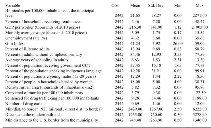
Table 3: Summary Statistics
Variable Obs Mean Std. Dev. Min Max
Homicides per 100,000 inhabitants at the municipal
level 2442 21.65 78.27 0.00 2271.00
Percent of households receiving remittances 2442 6.46 7.20 0.00 48.47 GDP per worker (thousands of 2010 pesos) 2442 216.30 841.90 1.12 21903.00 Monthly average wage (thousands 2010 prices) 2442 3.09 1.75 0.17 15.54 Unemployment rate (%) 2442 4.32 3.60 0.00 35.68
Gini Index 2442 41.24 3.92 26.00 59.00
Percent of illiterate adults 2442 13.94 9.69 0.83 58.79 Percent of adults without completed primary 2442 34.46 12.93 3.53 77.59 Average years of schooling in adults 2442 6.63 1.53 2.31 13.30 Percent of population receiving government CCT 2442 32.45 15.18 1.63 77.73 Percent of the population speaking indigenous language 2442 19.28 31.21 0.00 99.91 Percent of population are young males (15-29 years) 2442 12.29 1.44 2.22 18.50 Percent of people in households headed by women 2442 18.00 5.00 4.00 38.31 Density, urban area (thousands of inhabitants/km2) 2442 5.82 7.32 0.08 95.80 Convicted of murder per 100,000 inhabitants 2442 3.79 9.38 0.00 122.50 Sentenced for drug trafficking per 100,000 inhabitants 2442 9.28 34.46 0.00 1198.00 Number of drug cartels 2442 0.69 1.46 0.00 12.00 Min(dist. to border 1920 railroad , direct dist. to border) 2442 2429.00 1267.00 2.50 6222.00 Distance to the modern railroads 2442 1465.00 750.60 0.50 5278.00 Min distance to the U.S. border from the municipality 2442 748.40 263.90 0.50 1346.00
The dataset is a cross-section of Mexico at the municipal level for the year 2010. Summarized statistics of these variables are presented in Table 3. The dataset was compiled from different sources. To avoid the problem of underreporting of official crime statistics (such as robbery rates), we use homicides as a good measure of the level of crime, since homicide is less underreported. The number of homicides per 100,000 inhabitants was gathered from the Sistema Estatal y Municipal de Base de Datos (SIMBAD), an online query system of the National Institute of Statistics and Geography (Instituto Nacional de Estadística y Geografía—INEGI).4 The average number of homicides per 100,000 inhabitants is 21.65, with a standard deviation of 78 and a maximum of 2271. This high dispersion is the result of the influence of outliers (the 99th percentile is 246 homicides), mainly from municipalities where drug activity was intense in
11
that year, such as in cities located in the states of Nuevo Leon, Chihuahua, Sinaloa, Sonora, and Tamaulipas (Figure 2). Also, about 43 percent of municipalities reported no homicides.
Figure 2: Homicides per 100,000 Inhabitants, Mexico 2010
Mexico has seen an increase in violent crimes in recent years, with a homicide rate in 2010 that was more than twice that of 2005 (see Figure 3). From 2000 to 2007, the average homicide rate was around 10, but this pattern has changed. Since 2007, there has been a continuous increase in homicides that can be attributed to illegal drug trafficking. With information published by the Mexican Presidency in 2011, Figure 3 also presents the number of drug-related homicides.5 The overall homicide rate begins to increase rapidly with a similar slope as the rate of homicides related to drug trafficking.
5 These are homicides that had a relation with illegal drug trade. There include executions (targeted homicides),
12
Figure 3: Homicides Rate versus Drug-related Homicide Rate
.
The demographic and housing characteristics come from the 2010 Population and Housing Census, conducted by INEGI. Our main variable of interest is remittances, which we measure as the percentage of households in each municipality receiving remittances. These data come from an extended questionnaire that included questions about immigration and remittances. This questionnaire was designed to be representative at the municipal level and covers about 2.9 million households. On average, 6.46 percent of households in a municipality receive remittances.6 Around 2 percent of municipalities do not have households receiving remittances, and the top 10 percent of municipalities, more than 16 percent of households receive remittances. The municipalities with the highest number of households receiving remittances are located in the west and north-central states of the country (see Figure 4).
GDP per worker at the municipal level is reported by SIMBAD. It was calculated with information from the National Economic Census 2008. Unfortunately, there is no information for 2010, but measuring income is a good proxy. The average GDP per worker was nearly 216,000 Mexican pesos in 2010. Gini index data at the municipal level come from the Consejo Nacional de Evaluación de la Política de Desarrollo Social (CONEVAL). Data on the monthly average wage, illiterate adults, average years of schooling, the population receiving conditional cash
13
transfers (CCT), the population of young males, household headed by women, and the unemployment rate also come from the 2010 census.
Figure 4: Percentage of Household Receiving Remittances, Mexico 2010
With respect to apprehension, conviction, and severity of punishment, SIMBAD provides data on the number of murderers convicted and sentenced for drug trafficking. The average number of persons convicted and sentenced per 100,000 inhabitants is 3.79 and 9.28, respectively. To control for the presence of drug cartels in every municipality, we use the information calculated by Coscia and Viridiana (2012), who use online newspapers and blogs to identify the areas of operation of Mexican drug trafficking organizations. The average number of cartels is 0.69, with almost 29 percent of municipalities without the presence of cartels. Only the top 1 percent of municipalities has more than seven cartels. We also take into account the direct distance to the U.S. border from every municipality and the distance to modern railroads (1998 rail lines). These data come from Demirguc-Kunt et al. (2011), and the idea is that the closer a municipality is to the U.S. border, the higher the price of the drug. For this reason, in municipalities located closer to the border, the homicide rate will be higher due to the higher value of the loot. As mentioned before, drug-related murders are a significant fraction of the total rate.
14
5. Results of the Effect of Remittances on Crime
Table 4 reports our empirical specification using the Tobit model. Columns 4.1 to 4.4 report a negative and significant correlation between remittances and the homicide rate. In column 4.1, the relation is a reduction in the homicide rate by 0.018 percent when the number of households receiving remittances increases by 1 percent. In this specification, we only controlled for state-level dummies. However, the effect continues to be negative, even when we control for economic, demographic, and deterrence variables.
Column 4.2 includes wealth, labor, and income distribution controls. GDP per worker has the expected sign, but it is almost not significant. Contrary to what the theory says, the average wage and the unemployment rate have an opposite sign, although in the case of unemployment it is not significant. These biased results may be due to the fact that we only observe variation in municipalities and not over time. The Gini index indicates a significant increase in the homicide rate in municipalities with greater inequality. This result is in line with the conclusion of Fajnzylber, Lederman, and Loayza (1998).
In column 4.3, we control for some economic and demographic series. One main factor that affects crime is level of schooling in the community. Our three controls of schooling have the expected sign but are not significant. As reported by Chioda, De Mello, and Soares (2012) and Camacho and Mejia (2013), we observe a negative impact of a CCT program on the crime rate. With regard to the effect of indigenous people, there is a reduction in homicides if the share of the indigenous population is higher. The share of young males is related to an increase in homicides, as expected. We also control for mothers as heads of household. In the absence of the father or family disintegration (which could be because the father emigrated abroad), the young members may have an incentive to get involved in criminal activities or gangs. We observe a rise in the homicide rate as a result of this fact. Related to the effect of urban society, we observe higher crime rates in municipalities with higher population density in urban areas (1000 inhabitants per square kilometer).
15
Table 4: Tobit Estimation between Remittances and Crime Dependent variable:
Log(homicides per 100,000 inhabitants) at the municipal level
(4.1) (4.2) (4.3) (4.4) Tobit Tobit Tobit Tobit
Percent of households receiving remittances -0.018*** -0.011** -0.019*** -0.018*** (0.004) (0.004) (0.005) (0.005) GDP per worker (thousands of 2010 pesos) -0.000* -0.000 -0.000 (0.000) (0.000) (0.000) Monthly average wage (thousands of 2010 pesos) 0.126*** 0.077*** 0.070**
(0.016) (0.029) (0.029)
Unemployment rate (%) -0.002 -0.008 -0.008
(0.008) (0.008) (0.008)
Gini Index 0.049*** 0.048*** 0.049***
(0.006) (0.007) (0.007)
Percent of illiterate adults 0.009 0.008
(0.009) (0.009) Percent of adults without completed primary 0.009 0.008
(0.010) (0.010) Average years of schooling in adults -0.097 -0.116 (0.074) (0.075) Percent of population receiving government CCT -0.020*** -0.020***
(0.003) (0.003) Percent of the population speaking indigenous
language
-0.004*** -0.004*** (0.002) (0.002) Percent of population are young males 0.048** 0.045* (0.024) (0.024) Percent of people in households headed by women 0.026*** 0.024***
(0.007) (0.007) Density, considering urban municipal area 0.016*** 0.016***
(0.004) (0.004) Convicted of murder per 100,000 inhabitants 0.004
(0.003) Sentenced for drug trafficking per 100,000 inhabitants -0.000 (0.001)
Number of drug cartels 0.047***
(0.015)
Dummy by state level Yes Yes Yes Yes
Observations 2,442 2,442 2,442 2,442
Pseudo R2 0.09 0.10 0.12 0.13
Marginal effects at the mean. Robust standard errors in parentheses. *** p<0.01, ** p<0.05, * p<0.1.
We include some deterrence and drug controls in column 4.4. In both cases, the number of people sentenced for murder and drug trafficking is not significant. This may be a sign that punishment by the judicial system is not deterring criminal activities. On the other hand, there is a positive relationship between the number of drug cartels and the homicide rate. For each additional cartel, there is an increase in the homicide rate of about 0.05 percent. Table 4 reports a
16
negative impact of remittances on homicides, but these results ignore the possible endogeneity of remittances. As mentioned in the previous section, there are several sources of endogeneity, such as reverse causality or unobservable variables. To address these potential biases, we use the instrumental variable approach.
Our instrument, based on the distance of each municipality to the rail network in 1920 plus the distance of the railroad from that point to the border, is a variable that is correlated to the flow of migration and remittances at the present time. However, to meet the exclusion restriction, we need to establish that the historical rail network is not affecting the present crime rate, at least through the income effect channel of remittances. Commercial and economic activities might be linked to municipalities where modern railroads pass, and this commercial dynamism could be related to higher crime rates. To isolate this effect, we follow Demirguc-Kunt et al. (2011) and control for the distance of the municipality to the nearest modern rail line in 1998. Railroad development after 1920 will have a more direct effect on crime but will have less effect on patterns of migration.
Table 5 present the first-stage results. Here we study the relationship between remittances and the distance to the U.S. border along the rail network in 1920, after controlling for other socioeconomic characteristics and the modern railroad network. We use as the dependent variable the percentage of households receiving remittances, and as predictors, the minimum between the distance to the border along the 1920 railroad lines or the direct distance to the border; the distance to the modern railroad network; and a series of economic, demographic, and drug-related controls.
17
Table 5: First-stage Estimates of the Effect of the Minimum Distance in 1920 on Remittances
Dependent variable: percent of households receiving remittances at the municipal level
(5.1) (5.2) (5.3) (5.4) Instrument
Min(distance to border along 1920 railroad , direct distance to border) -0.0060*** -0.0059*** -0.0044*** -0.0044*** (0.0006) (0.0006) (0.0005) (0.0005) Controls
GDP per worker (thousands of 2010pesos) -0.0003* -0.0001 -0.0001 (0.0001) (0.0001) (0.0001) Monthly wage (thousands of 2010pesos) -0.7005*** -0.5896*** -0.5647***
(0.0842) (0.1505) (0.1503)
Unemployment rate 0.1084** 0.0511 0.0509
(0.0430) (0.0372) (0.0372)
Gini Index -0.0512 0.0261 0.0239
(0.0325) (0.0352) (0.0351)
Percent of illiterate adults -0.2345*** -0.2307***
(0.0406) (0.0410) Percent of adults without completed primary 0.2367*** 0.2361***
(0.0473) (0.0473) Average years of schooling in adults -0.9713*** -0.9377***
(0.3589) (0.3601) Percent of population receiving government CCT -0.0925*** -0.0925***
(0.0187) (0.0187) Percent of the population speaking indigenous language -0.0083 -0.0083
(0.0074) (0.0074) Percent of population are young males -0.9808*** -0.9742***
(0.1187) (0.1192) Percent of people in households headed by women 0.3890*** 0.3942***
(0.0337) (0.0336) Density, considering urban municipal's area -0.0384** -0.0376**
(0.0164) (0.0164)
Convicted of murder per 100,000 inhabitants -0.0095
(0.0148) Sentenced for drug trafficking per 100,000 inhabitants -0.0031
(0.0028)
Number of drug cartels -0.1362
(0.1067) Distance to the modern railroads (1998) -0.0001 -0.0009* -0.0003 -0.0003
(0.0005) (0.0005) (0.0004) (0.0004) Minimum distance to the U.S. border from the municipality 0.0259*** 0.0267*** 0.0197*** 0.0196***
(0.0028) (0.0028) (0.0024) (0.0024)
Constant 6.3818*** 14.2668*** 21.9586*** 22.1041***
(2.3017) (2.7075) (4.2034) (4.2258)
Dummy by state level Yes Yes Yes Yes
Observations 2,442 2,442 2,442 2,442
R-squared 0.3094 0.3326 0.4979 0.4988
Kleibergen-Paap under identification test 94.81 95.91 76.14 76.22 Cragg-Donald F statistic for weak instruments 130.60 131.50 91.08 91.08 Kleibergen-Paap F statistic for weak instruments 109.86 109.62 82.00 82.01
Robust standard errors in parentheses. *** p<0.01, ** p<0.05, * p<0.1.
18
Columns 5.1 through 5.4 show a strong and significant relationship between the instrumental variable and the percentage of households receiving remittances. The results show that every kilometer is associated with a decrease in the percentage of households receiving remittances of at least 0.004 percentage points. This means that municipalities near the historic rail network have more households receiving remittances. We also observed that the effect of the modern rail network is not significant to the remittances received in each municipality. These results support the idea that historically the rail network was the determinant factor in establishing migration patterns to the United States. With respect to the validity of the instrument, the Cragg-Donald F and Kleibergen-Paap tests of weak identification reject the null hypothesis that the instrument is weak.
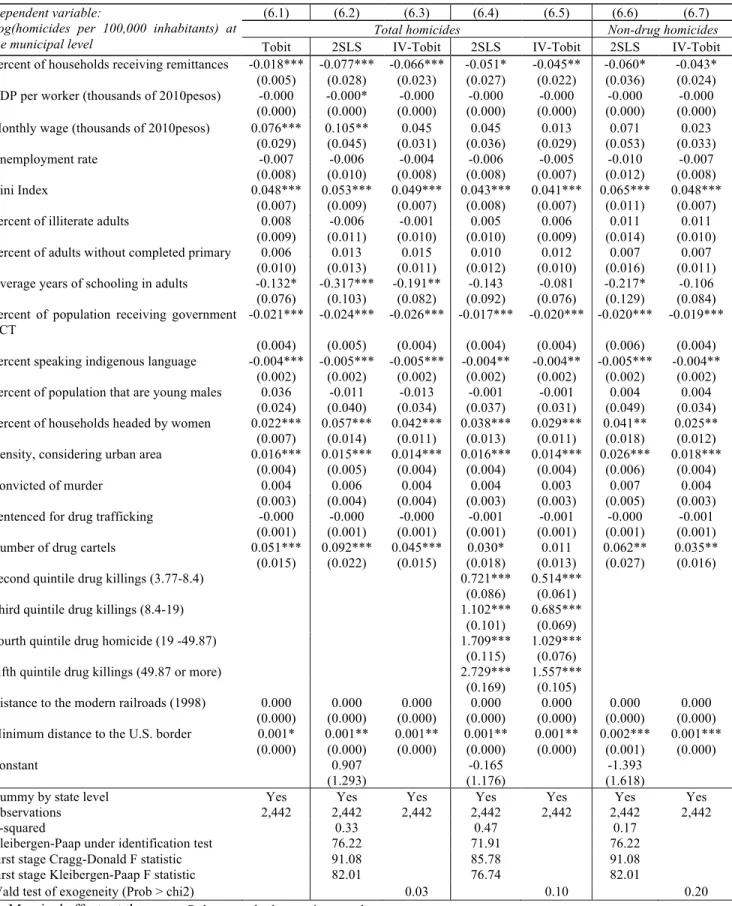
The second stage of our analysis attempts to determine the effect of remittances on crime. Table 6 contains the estimates of the effect of remittances on the homicide rate. The Tobit estimate in column 6.1 shows that each 1 percent increase in households receiving remittances is related to a 0.02 percent reduction in the homicide rate. The instrumental variable is used in column 6.2 and 6.3. When we instrument for remittances, we find a larger negative impact of remittances on the homicide rate. The 2SLS show a reduction in homicides of 0.08 percent, but the IV-Tobit in column 6.3 show an effect of 0.07 percent. The difference may be explained by the econometric specification, because the Tobit model takes into account that the homicide data is truncated.
To take into account the increase in drug-related homicides, in columns 6.1 to 6.3 we control for the number of drug cartels. The homicide rate increases by at least 0.04 percent for each drug cartel operating in the municipality. As mentioned above, this is a measure of the degree of confrontation among criminal groups. Also, we control for the minimum distance of the municipality to the U.S. border. An additional kilometer to the border is associated with an increase in the homicide rate of at least 0.001 percent.
19
Table 6: IV Second-stage Estimates of the Impact of Remittances on Homicides Dependent variable:
Log(homicides per 100,000 inhabitants) at the municipal level
(6.1) (6.2) (6.3) (6.4) (6.5) (6.6) (6.7)
Total homicides Non-drug homicides
Tobit 2SLS IV-Tobit 2SLS IV-Tobit 2SLS IV-Tobit Percent of households receiving remittances -0.018*** -0.077*** -0.066*** -0.051* -0.045** -0.060* -0.043*
(0.005) (0.028) (0.023) (0.027) (0.022) (0.036) (0.024) GDP per worker (thousands of 2010pesos) -0.000 -0.000* -0.000 -0.000 -0.000 -0.000 -0.000 (0.000) (0.000) (0.000) (0.000) (0.000) (0.000) (0.000) Monthly wage (thousands of 2010pesos) 0.076*** 0.105** 0.045 0.045 0.013 0.071 0.023
(0.029) (0.045) (0.031) (0.036) (0.029) (0.053) (0.033) Unemployment rate -0.007 -0.006 -0.004 -0.006 -0.005 -0.010 -0.007 (0.008) (0.010) (0.008) (0.008) (0.007) (0.012) (0.008) Gini Index 0.048*** 0.053*** 0.049*** 0.043*** 0.041*** 0.065*** 0.048***
(0.007) (0.009) (0.007) (0.008) (0.007) (0.011) (0.007) Percent of illiterate adults 0.008 -0.006 -0.001 0.005 0.006 0.011 0.011
(0.009) (0.011) (0.010) (0.010) (0.009) (0.014) (0.010) Percent of adults without completed primary 0.006 0.013 0.015 0.010 0.012 0.007 0.007
(0.010) (0.013) (0.011) (0.012) (0.010) (0.016) (0.011) Average years of schooling in adults -0.132* -0.317*** -0.191** -0.143 -0.081 -0.217* -0.106 (0.076) (0.103) (0.082) (0.092) (0.076) (0.129) (0.084) Percent of population receiving government
CCT -0.021*** -0.024*** -0.026*** -0.017*** -0.020*** -0.020*** -0.019*** (0.004) (0.005) (0.004) (0.004) (0.004) (0.006) (0.004) Percent speaking indigenous language -0.004*** -0.005*** -0.005*** -0.004** -0.004** -0.005*** -0.004**
(0.002) (0.002) (0.002) (0.002) (0.002) (0.002) (0.002) Percent of population that are young males 0.036 -0.011 -0.013 -0.001 -0.001 0.004 0.004
(0.024) (0.040) (0.034) (0.037) (0.031) (0.049) (0.034) Percent of households headed by women 0.022*** 0.057*** 0.042*** 0.038*** 0.029*** 0.041** 0.025** (0.007) (0.014) (0.011) (0.013) (0.011) (0.018) (0.012) Density, considering urban area 0.016*** 0.015*** 0.014*** 0.016*** 0.014*** 0.026*** 0.018***
(0.004) (0.005) (0.004) (0.004) (0.004) (0.006) (0.004) Convicted of murder 0.004 0.006 0.004 0.004 0.003 0.007 0.004
(0.003) (0.004) (0.004) (0.003) (0.003) (0.005) (0.003) Sentenced for drug trafficking -0.000 -0.000 -0.000 -0.001 -0.001 -0.000 -0.001 (0.001) (0.001) (0.001) (0.001) (0.001) (0.001) (0.001) Number of drug cartels 0.051*** 0.092*** 0.045*** 0.030* 0.011 0.062** 0.035** (0.015) (0.022) (0.015) (0.018) (0.013) (0.027) (0.016) Second quintile drug killings (3.77-8.4) 0.721*** 0.514***
(0.086) (0.061) Third quintile drug killings (8.4-19) 1.102*** 0.685***
(0.101) (0.069) Fourth quintile drug homicide (19 -49.87) 1.709*** 1.029***
(0.115) (0.076) Fifth quintile drug killings (49.87 or more) 2.729*** 1.557***
(0.169) (0.105)
Distance to the modern railroads (1998) 0.000 0.000 0.000 0.000 0.000 0.000 0.000 (0.000) (0.000) (0.000) (0.000) (0.000) (0.000) (0.000) Minimum distance to the U.S. border 0.001* 0.001** 0.001** 0.001** 0.001** 0.002*** 0.001***
(0.000) (0.000) (0.000) (0.000) (0.000) (0.001) (0.000)
Constant 0.907 -0.165 -1.393
(1.293) (1.176) (1.618)
Dummy by state level Yes Yes Yes Yes Yes Yes Yes
Observations 2,442 2,442 2,442 2,442 2,442 2,442 2,442
R-squared 0.33 0.47 0.17
Kleibergen-Paap under identification test 76.22 71.91 76.22
First stage Cragg-Donald F statistic 91.08 85.78 91.08
First stage Kleibergen-Paap F statistic 82.01 76.74 82.01
Wald test of exogeneity (Prob > chi2) 0.03 0.10 0.20
Marginal effects at the mean. Robust standard errors in parentheses. *** p<0.01, ** p<0.05, * p<0.1.
20
Another way of separating the impact of drug trafficking on the homicide rate is to use the data on drug-related homicides published by the Mexican Presidency for 2010. With these data, we classified the municipalities with homicides into five groups of dummy variables.7 Columns 6.4 and 6.5 present the results. Each dummy is highly significant, and when a municipality belongs to a higher quintile it has a greater impact on the homicide rate. Under these controls, the effect of remittances decreases, but it remains negative and significant. Every 1 percent increase in households receiving remittances reduces the homicide rate by 0.05 percent. Interestingly, the effect of the number of cartels became not significant, which means that the dummy variables are capturing the effect of drug trafficking.
A more direct way to separate the effect of drug trafficking is to subtract from the total number of homicides reported by INEGI the number of drug-related homicides reported by the Presidency.8 In columns 6.6 and 6.7, we use “homicide rate without drug trafficking” as the dependent variable. Once again, the instrumental estimations present a negative and significant impact of remittances on crime, and they are of similar magnitude to our previous results. Even subtracting the drug-related homicides, the number of cartels has a positive and significant influence on crime. This may be a side effect of drug trafficking on other criminal activities.
The impact of the economic and demographic controls on the crime rate remains similar to those discussed in Table 4. Nonetheless, it is worth commenting on some of them. GDP per worker remains negative but not significant. In the 2SLS, wages have a significant positive effect, but in the IV estimations this effect is no longer significant. Unemployment remains not significant. Years of schooling shows a more important, significant, and negative impact on the crime rate. Both the percentage of households receiving CCT and speaking indigenous languages have a negative and very significant impact. Municipalities with more households headed by women and a high urban density observe a higher crime rate. As mentioned before, the effect of the single mother household may be related to the rupture of family unit or disintegration.
7 The dummy variables were created in base of 5 quintiles with the municipalities with homicides related to drugs. 8 In 6 percent of municipalities, the number of homicides reported by the Presidency was higher than the data reported by
21
6. The Effect of Remittances on Other Crimes
One concern about using the homicide rate as a proxy for the crime level is that this rate might not be related to other crimes. We report additional estimations of the effect of remittances on other crimes: street robbery, extortions, burglary, and car theft. Using data from the Encuesta Nacional de Victimización y Percepción sobre Seguridad Pública 2011 (ENVIPE), conducted by ENEGI, we calculated the number of crimes in each category per 100,000 inhabitants. The survey asked whether people had been victims of crimes in 2010, so we can relate these rates to census data at the municipal level.
A major concern of using the ENVIPE 2011 is that it is not representative at the municipal level. For this reason, our sample is limited to municipalities with 50 or more households. We chose this number as a very demanding threshold, but the results are similar using a lower or higher cutoff. In this way, information was obtained on only 800 of the 896 municipalities in the survey. The summary statistics are presented in Table A1 in the appendix. For 2010, we observe that on average, at the municipal level, the most frequent crime was extortions, with 4,103 cases per 100,000 inhabitants, followed by burglary, with a rate of 3,620; street robbery, with 3,262; and finally, car theft, with 626 cases. The last column of the summary shows that a significant percentage of municipalities reported no crimes; therefore, data is left-truncated and it is necessary to use a Tobit model for a better fit.
Table 7 present the second stage of the 2SLS and IV-Tobit models and contains the estimates of the effect of remittances on the logarithm of the crime rates. As in Table 6, we instrument for remittances in each column using the distance from the municipality to the U.S. border along the rail network in 1920. We find a negative impact of remittances in three of the crime rates, with only street robbery being significant. In column 7.1, the 2SLS result shows a reduction of 0.19 percent in street robbery with each 1 percent increase in the number of households receiving remittances at the municipal level. This effect is larger when we use the IV-Tobit model, with an impact of 0.41 percent of remittance on the reduction of street robbery. The lack of significance in the other rates could be related to the fact that we only have information on a third of the municipalities in Mexico. However, we observe some evidence of the effect of remittances on the reduction of other crime rates.
22
Table 7: IV-Tobit Second-stage Estimates of the Impact of Remittances on Other Crimes
(7.1) (7.2) (7.3) (7.4) (7.5) (7.6) (7.7) (7.8)
Dependent variable: Street robbery Extortions Burglary Car theft
Log(crime per 100,000 inhabitants) at the municipal level
2SLS IV-Tobit 2SLS IV-Tobit 2SLS IV-Tobit 2SLS IV-Tobit % of households receiving remittances -0.189* -0.411** -0.082 -0.134 -0.085 -0.131 0.109 0.188
(0.108) (0.198) (0.109) (0.180) (0.118) (0.181) (0.072) (0.197) GDP per employee(thousands of pesos) -0.000*** -0.000** 0.000 -0.000 0.000 0.000 -0.000** -0.000
(0.000) (0.000) (0.000) (0.000) (0.000) (0.000) (0.000) (0.000) Wage per worker (2010 prices) 0.012 0.006 -0.040 -0.084 -0.055 -0.119 0.071 0.003
(0.062) (0.116) (0.067) (0.113) (0.075) (0.123) (0.048) (0.122) Unemployment rate 0.049* 0.104* 0.054* 0.088* 0.010 0.018 -0.027 -0.047
(0.029) (0.058) (0.029) (0.045) (0.031) (0.049) (0.018) (0.049)
Gini Index 0.019 0.047 0.009 0.019 0.027 0.047 -0.003 0.035
(0.017) (0.033) (0.018) (0.031) (0.021) (0.032) (0.015) (0.035) Percent of illiterate adults 0.000 0.004 0.051 0.078 -0.029 -0.069 0.041** 0.067
(0.030) (0.062) (0.032) (0.056) (0.033) (0.054) (0.016) (0.051) Percent of adults without completed
primary 0.005 0.001 0.026 0.041 0.034 0.063 0.012 0.055
(0.038) (0.074) (0.037) (0.063) (0.042) (0.065) (0.023) (0.067) Average years of schooling in adults -0.125 -0.387 0.362** 0.511* 0.217 0.360 0.455*** 0.893***
(0.166) (0.295) (0.163) (0.275) (0.196) (0.305) (0.103) (0.277) Percent of population receiving CCT -0.028*** -0.048*** -0.033*** -0.058*** -0.014 -0.024 -0.013** -0.069***
(0.009) (0.018) (0.010) (0.018) (0.010) (0.016) (0.006) (0.018) Percent speaking indigenous language -0.009 -0.021* -0.007 -0.013 -0.006 -0.009 0.001 -0.016
(0.006) (0.012) (0.006) (0.011) (0.007) (0.011) (0.004) (0.015) Percent of population that are young
males -0.183 -0.353 -0.042 -0.077 0.060 0.089 0.130 0.252
(0.119) (0.225) (0.123) (0.206) (0.133) (0.207) (0.083) (0.219) Percent of households headed by women 0.063 0.139 0.039 0.065 0.024 0.030 -0.054* -0.092
(0.050) (0.093) (0.048) (0.080) (0.055) (0.083) (0.033) (0.086) Density, considering urban area 0.009 0.014 -0.006 -0.008 0.002 0.005 0.015* 0.038* (0.012) (0.021) (0.014) (0.026) (0.012) (0.021) (0.008) (0.023) Convicted of murder -0.012 -0.030 0.004 0.015 -0.005 -0.003 0.004 0.027
(0.012) (0.027) (0.013) (0.022) (0.015) (0.024) (0.007) (0.021) Sentenced for drug trafficking. -0.001 -0.001 -0.002 -0.002 0.002 0.002 -0.003* -0.009**
(0.003) (0.006) (0.004) (0.006) (0.003) (0.004) (0.002) (0.005) Number of drug cartels 0.070* 0.055 0.023 0.018 0.032 0.044 0.119*** 0.181***
(0.038) (0.068) (0.038) (0.060) (0.044) (0.065) (0.033) (0.063) Distance to U.S. in 1998 railroads -0.000 -0.000 -0.000 -0.000 -0.001* -0.001* 0.000 -0.000
(0.000) (0.001) (0.000) (0.000) (0.000) (0.000) (0.000) (0.000) Minimum distance to the U.S. border 0.001 0.001 0.000 0.000 0.002* 0.002* 0.000 0.002
(0.001) (0.002) (0.001) (0.001) (0.001) (0.001) (0.001) (0.001)
Constant 10.213*** 5.300** 3.769 -0.447
(2.462) (2.565) (2.825) (1.657)
Dummy by state level Yes Yes Yes Yes Yes Yes Yes Yes
Observations 800 800 800 800 800 800 800 800
R-squared 0.244 0.208 0.159 0.185
Kleibergen-Paap under identification test 14.52 14.52 14.52 14.52 First stage Cragg-Donald F statistic 14.27 14.27 14.27 14.27 First stage Kleibergen-Paap F statistic 13.92 13.92 13.92 13.92
Wald test of exogeneity (Prob > chi2) 0.10 0.45 0.51 0.26
Marginal effects at the mean. Robust standard errors in parentheses. *** p<0.01, ** p<0.05, * p<0.1.
23
7. A State-level Panel
The problem with constructing remittance panel data at the local level is that there is no long time-series information. However, the Central Bank of Mexico reports quarterly on the amount of remittances received at the state level. The advantage of using a panel dataset is to control for the unobservable characteristics of the state over time. Once again, endogeneity between remittances and homicides is a major concern. To deal with this issue, we use two instrumental variables.
Following Orrenius, et al. (2009), we use U.S. wage growth9 and unemployment rates at the state level as instruments for remittances.10 There is a strong correlation between labor conditions in the United States and remittance flows. But this strategy leads to some important questions. What wage and unemployment rate is relevant for each Mexican state? Does the wage and unemployment rate of California or New York affect remittances received in Oaxaca? Using the estimations of Conapo (2005) and the data of the Mexican National Survey (ENE11) 2002, we
construct time-invariant weights of the percent of Mexicans from each state of Mexico in each U.S. state. Therefore, our weighted average index of wage growth and unemployment is based on equation 2:
𝐼𝑛𝑑𝑒𝑥!" = 𝑀𝑖𝑔𝑟𝑎𝑛𝑡!" !"
!!!
∗ 𝑂𝑢𝑡𝑐𝑜𝑚𝑒!" (2)
where 𝐼𝑛𝑑𝑒𝑥!" represents the wage growth (or unemployment) relevant to the Mexican state i in the quarter t; 𝑀𝑖𝑔𝑟𝑎𝑛𝑡!" represents the share of migrants of Mexican state i who live in U.S.
state j and 𝑂𝑢𝑡𝑐𝑜𝑚𝑒!" is wage growth (or unemployment) in U.S. state j in the quarter t. The
U.S. state-level data on wages comes from the Quarterly Census of Employment and unemployment rates from the U.S. Bureau of Labor Statistics.
9 We use the wage growth in place of the wage level because in an economic recession the labor market adjusts mainly
through the number of workers, instead the level of wage. It is calculated as the annual percentage change of wage in the same quarter.
10 We cannot use the instrument of the distance along the 1920 rail network because it does not have variation over time
and it is calculated at municipal level.
11 For 2002, this survey includes a module that collected information about the migration pattern, origin, and destination
24
Table 8 reports first-stage regressions and a battery of econometrics test performed to assess the validity of these instruments. We use as a dependent variable the quarterly state-level remittances per capita12 and as predictors, the U.S. weighted wage growth, the U.S. weighted unemployment rate, and other controls.
Table 8: IV First-stage Estimations of U.S. Wages and Unemployment on Remittances
(quarterly state panel, 2003–2010)
Dependent variable:
Remittances per capita (real US $) at the state level
(8.1) (8.2) (8.3) (8.4)
Instruments
U.S. quarterly wage growth 1.403*** 1.135*** 0.945*** 0.881*** (0.153) (0.118) (0.0957) (0.101) U.S. quarterly unemployment rate -1.534*** -2.219*** -1.880*** -2.218***
(0.285) (0.185) (0.436) (0.451) Controls
State real wage in Mexico 0.810*** 0.680*** 0.512** (0.139) (0.232) (0.246) State unemployment rate in Mexico 2.057*** 1.956*** 1.417** (0.323) (0.629) (0.610)
State years of schooling -7.033*** -6.294***
(1.043) (1.063)
Municipal average drug cartels 3.017***
(0.944) Constant 61.94*** 37.04*** 101.8*** 98.60*** (1.874) (3.960) (9.250) (10.22) Observations 1,024 1,024 1,024 1,024 R-squared 0.305 0.357 0.415 0.441 Number of states 32 32 32 32
Anderson LM Under identification test 302.73 267.21 204.69 232.58 Cragg-Donald F statistic for weak instruments 217.41 182.12 128.30 150.98 Sargan overidentification test 47.29 2.76 2.65 1.11 Sargan overidentification test (p-value) 0.00 0.10 0.10 0.29 Robust standard errors in parentheses (clustered at state level). Dummy fixed effect by state and dummy fixed effect by quarter. *** p<0.01, ** p<0.05, * p<0.1.
Columns 8.1 through 8.5 show a strong and significant correlation of both instrumental variables with the amount of remittances per capita received in each Mexican state. Furthermore, the Cragg-Donald F statistics always reject the null hypothesis that the instruments are weak. In the case of the Sargan tests, once we include other controls, we do not reject the null hypothesis that the errors are correlated with the explanatory variables. The reported regressions include
12 In real 2007 U.S. dollars, deflated using the CPI-W Q4 2007. The results are similar using remittances as millions of
25
state-level and quarterly fixed effects. Both instruments have the expected sign; U.S. wage growth is positively associated with the level of remittances per capita and the U.S. unemployment rate is negatively correlated.
Table 9: IV second stage estimations of remittances on homicide rate (quarterly state panel, 2003–2010)
Dependent variable:
homicides per 100,000 inhabitants
(9.1) (9.2) (9.3) (9.4) (9.5) (9.6) OLS IV-OLS OLS IV-OLS OLS IV-OLS Remittances per capita (real US $) 0.012 -0.051*** 0.015 -0.066*** 0.012 -0.055** (0.016) (0.019) (0.016) (0.024) (0.017) (0.022) State real wage in Mexico -0.276** -0.174*** -0.273** -0.174*** -0.288** -0.210***
(0.130) (0.057) (0.129) (0.057) (0.123) (0.056) State unemployment rate in Mexico 1.291** 1.225*** 1.284** 1.244*** 1.159* 1.094***
(0.557) (0.087) (0.559) (0.087) (0.622) (0.102) State years of schooling 0.198 -0.650* 0.234 -0.454
(0.283) (0.361) (0.299) (0.345)
Municipal average drug cartels 0.399 0.502***
(0.374) (0.168) Constant 4.888*** 5.742*** 2.916 12.268*** 2.884 10.573*** (1.383) (1.388) (2.571) (3.993) (2.586) (3.824) Observations 1,024 1,024 1,024 1,024 1,024 1,024 R-squared 0.23 0.20 0.23 0.18 0.23 0.20 Number of states 32 32 32 32 32 32
Anderson LM Under identification test 267.21 204.69 232.58 Cragg-Donald F statistic for weak instruments 182.12 128.30 150.98
Sargan overidentification test 2.76 2.65 1.11
Sargan overidentification test (p-value) 0.10 0.10 0.29 Robust standard errors in parentheses (OLS clustered at state level). Dummy fixed effect by state and dummy fixed effect by quarter. *** p<0.01, ** p<0.05, * p<0.1.
Table 9 contains the estimates of the effect of remittances per capita on homicides per 100,000 inhabitants. Column 9.1 shows that the OLS result of remittances is positive and not significant. When we use the instruments in column 9.2, the effect of remittances is negative and highly significant. Each additional real U.S. dollar of remittances per capita received reduces the homicide rate by 0.05 at the state level. One major concern of our identification strategy is that the U.S. business cycle is highly correlated with the Mexican business cycle. In a recession that affects both countries (such as the 2008–2009 global economic crisis), the deterioration of the Mexican economy may have increased criminal activities. Therefore, in column 9.2 we also include the state wage and state unemployment rate in Mexico. These data come from the
26
(ENOE), administered by INEGI.13 The summary statistics of the state-level data are presented
in the Table A2 of the appendix.
Comparing cross-sectional results, wage and unemployment are significant and have the expected signs. A higher wage level is correlated with less crime, and an elevated unemployment rate is correlated with more crime. We also included years of schooling at state level, calculated using the ENOE information. More educated states are associated with lower homicide rates. Finally, in columns 9.5 and 9.6, we control for the state average of the number of drug cartels that operate at municipal level. These data are yearly and were estimated by Cosia and Viridiana (2012). Once again, drug cartels have a positive and significant impact on the crime rate.
8. Conclusions
Remittances are an important source of income for many households and communities in Mexico, as well as the LAC region in general. Even though the economic literature related to remittances on households’ activities is abundant, it has not yet explored the effect of remittances on crime. Mexico is an excellent case study because both remittances and crime are relevant factors in the country. In this paper, we show that remittances from the United States reduce homicide rates. One of the mechanisms of transmission could be that remittances reduce poverty and thus discourage households from engaging in crime. Remittances may also allow them to invest more in education of the children, reducing the incentive to become delinquent. Moreover, previous studies show that remittances increase school enrollment and retention, which can be a channel of incapacitation that prevents young people from engaging in criminal activities. Another channel of influence could be that remittances are invested in economic activities that help create jobs for young people, preventing them from participating in crime. Future research should disentangle the contribution of these and other factors to explain how remittances affect crime.
We use municipal-level data for Mexico in 2010. Two major concerns rise in evaluating this impact: first, the presence of endogeneity between remittances and homicides originated by reverse causality and omitted factors, and second, violence related to drug trafficking. To address
13 ENE and ENOE are the quarterly national employment surveys produced by INEGI. The ENOE replace the ENE in
27
the first issue, we use the instrumental variable approach to deal with the endogeneity of remittances. The fact that early migration to the United States from Mexico is correlated with the historic railroad network allowed us to use the distance of each municipality to the U.S. border along the railroad network in 1920 as an instrument. With respect to the second concern, we use as a control the number of drug cartels in every municipality to separate out the effect of drug trafficking. With data on drug-related homicides, we group the municipalities in quintiles and estimate the impact of remittances controlling for these groups. Finally, we subtract drug-related homicides from total homicides to eliminate the effect of these criminals groups.
In the estimations, after using the instrument and controlling for economic, demographic and drug-trafficking variables, we find evidence that remittances have a negative impact on the number of homicides. An increase of 1 percent of the households receiving remittances reduces the homicide rate by at least 0.04 percent.
Additionally, we use other types of crime data to evaluate the impact of remittances at the municipal level. We observe a 0.19 percent reduction in street robbery related to a 1 percent increase in the number of households receiving remittances. Finally, we use data on the amount of remittances per capita received in each state from 2003 to 2010 to create a dataset panel. To address the endogeneity of remittances in this state panel, we construct two instruments: a weighted wage growth and a weighted unemployment rate in United States. Both variables are strong predictors of remittances per capita received in Mexican states. The state panel estimations present a negative impact of remittances on the homicide rate.
28
References
Alcaraz, C., D. Chiquiar, and A. Salcedo. 2012. “Remittances, Schooling, and Child Labor in Mexico.” Journal of Development Economics 97(1): 156–65.
Antman, F. 2012. “Gender, Educational Attainment, and the Impact of Parental Migration on Children Left Behind.” Journal of Population Economics 25(4): 1187–1214.
Becker, G. 1968. "Crime and Punishment: An Economic Approach.” Journal of Political Economy 76.
Berthelon, M. E., and D. I. Kruger. 2011. “Risky Behavior among Youth: Incapacitation Effects of School on Adolescent Motherhood and Crime in Chile.” Journal of Public Economics
95(1): 41–53.
Bignon, V., E. Caroli. and R. Galbiati. 2011. “Stealing to Survive: Crime and Income shocks in 19th Century France.” Paris: Cepremac. Available at:
http://www.cepremap.fr/depot/docweb/docweb1111.pdf
Calderón, G., B. Magaloni, and G. Robles. 2013. “The Economic Costs of Drug-Trafficking Violence in Mexico.” Working Paper, Center on Democracy, Development and the Rule of Law. Palo Alto, CA: Stanford University.
Camacho, A., and D. Mejía. 2013. “Las externalidades de los programas de transferencias condicionadas sobre el crimen: El caso de Familias en Acción en Bogotá.” IDB Working Paper 406. Institutions for Development Sector. Washington, DC: Inter-American Development Bank.
Cameron, A.C., and P. K. Trivedi. 2009. “Microeconometrics Using Stata.” Stata Press.
Castillo, J.C., D. Mejia, and P. Restrepo. 2013. “Illegal Drug Markets and Violence in Mexico: Causes beyond Calderon.” Unpublished.
Avaible at: http://cie.itam.mx/SEMINARIOS/Marzo-Mayo_2013/Mejia.pdf
Chiapa, C., and J. Viejo. 2012. “Migration, Sex Ratios and Violent Crime: Evidence from Mexico’s Municipalities.” NEUCDC Conference November 2012. Hanover, NH:
Dartmouth College. Available at:
29
Chioda, L., J. M. P. De Mello, and R. Soares. 2012. “Spillovers from Conditional Cash Transfer Programs: Bolsa Família and Crime in Urban Brazil.” Textos para discussao 599. Rio de Janeiro, Brazil: Department of Economics PUC-Rio.
Coatsworth, J. 1972. “The Impact of Railroads on the Economic Development of Mexico, 1877– 1910” Ph.D. Dissertation. Madison, WI: University of Wisconsin.
Conapo 2005. “Migración México-Estados Unidos:Panorama regional y estatal.” Consejo Nacional de Población. Secretaria de Gobernación. Gobierno de Mexico. Mexico D.F.
Available at:
http://www.conapo.gob.mx/work/models/CONAPO/migracion_internacional/panorma_re gional_estatal/02.pdf
Corbacho, A., and M. Ruiz-Vega. 2013. “The Dynamics of Crime in Latin America and the Caribbean.” Washington, DC: Inter-American Development Bank. Unpublished.
Coscia, M. and R. Viridiana. 2012. “Knowing Where and How Criminal Organizations Operate Using Web Content.” In CIKM’12, October 29–November 2, 2012, Maui, HI, USA. Copyright 2012 ACM 978-1-4503-1156-4/12/10.
Dean, Y. 2008. “International Migration, Remittances and Household Investment: Evidence from Philippine Migrants' Exchange Rate Shocks.” Economic Journal, Royal Economic Society 118 (528): 591–630.
Demirgüç-Kunt, A., E. Lopez, M. Martínez, and C. Woodruff. 2011. “Remittances and Banking Sector Breadth and Depth: Evidence from Mexico.” Journal of Development Economics
95(2): 229–41.
Fajnzylber, P., D. Lederman, and N. Loayza. 1998. “Determinants of Crime Rates in Latin America and the World, an Empirical Assessment.” World Bank Latin American and Caribbean Studies. Washington, DC: World Bank.
Fella, G. and G. Gallipoli. 2008. “Education and Crime over the Life Cycle.” Working Paper 630. London, United Kingdom: Queen Mary University of London.
Gordon H. and C. Woodruff. 2003. “Emigration and Educational Attainment in Mexico.”. San Diego, CA: University of California, San Diego. Unpublished.
Jacob, B.A., and J. Ludwig. 2010. “The Effects of Family Resources on Children's Outcomes.” Working Paper. Ann Arbor, MI: University of Michigan.