Long-term government debt and household
portfolio composition
AndreasTischbirek
Department of Economics, HEC Lausanne, University of Lausanne
Formal dynamic analyses of household portfolio choice in the literature focus on holdings of equity and a risk-free asset or bonds of different maturities, neglect-ing the interdependence of the decisions to invest in equity, short-term and long-term bonds made by households. Data from the Survey of Consumer Finances is used to derive stylized facts about participation in the long-term government-debt market and conditional portfolio shares. To explain the mechanisms under-lying these facts, I draw on a life-cycle model in which investors have access to three financial assets—equity, long-term debt, and a riskless short-term bond— and are exposed to uninsurable idiosyncratic risk through nonfinancial income as well as aggregate risk through the asset returns. An application shows that the low Treasury returns observed in the US between 2009 and 2013 have quantita-tively significant yet transitory effects on the composition of household portfo-lios. In combination with the observed rise in stock returns, they lead to persis-tent changes in the participation rate, the conditional portfolio shares, and the distribution of wealth.
Keywords. Dynamic portfolio choice, life cycle, long-term government debt, asset-market participation, survey of consumer finances.
JELclassification. D10, D15, E21, G11.
1. Introduction
Analyses of portfolio choice over the life cycle generally focus on holdings of stock and a risk-free asset, not taking into account the significant positions of long-term govern-ment debt that can be found in household portfolios. With short-term nominal interest rates close to the zero lower bound in Europe and the US in the aftermath of the the Fi-nancial Crisis of 2007 to 2009, central banks have purchased large amounts of long-term debt as a part of their unconventional monetary policy programs. In this context, the role that long-term bonds play in household portfolios and the motives for rebalancing portfolios in response to return shocks have become of considerable interest. Using a life-cycle model in which agents can invest in three financial assets—stocks, long-term government debt, and a riskless asset—this paper studies the decision to participate in
Andreas Tischbirek:andreas.tischbirek@unil.ch
I would like to thank Guido Ascari, Wouter den Haan, Martin Ellison, Elisa Faraglia, Francisco Gomes, Charles Gottlieb, Winfried Koeniger, Pascal St-Amour, as well as a number of seminar and conference participants for helpful comments and discussions. Financial support from the Royal Economic Society is gratefully acknowledged.
© 2019 The Author. Licensed under the Creative Commons Attribution-NonCommercial License 4.0. Available athttp://qeconomics.org.https://doi.org/10.3982/QE836
financial markets and the composition of household portfolios over the course of the life cycle with a focus on the role of long-term government debt.
Stylized facts are derived based on a data set constructed from seven consecutive waves of the Survey of Consumer Finances (SCF). The joint existence of birth cohort, time, and age influences on the participation rate and the respective portfolio shares conditional on participation result in a well-known identification problem.1Using three different identification strategies, two from the literature and one novel, a latent vari-able model with a participation equation is estimated. The standard approach based on cohort restrictions performs the least well. The remaining two, although distinct, give nearly identical results. Similar to participation in the stock market, participation in the market for long-term debt takes an inverse U-shape. While the conditional portfo-lio share of stocks is declining with age, the conditional share of long-term government debt is moderately increasing until the age of around55and significantly lowered from about65onwards.2 Long-term bond holdings and holdings of the riskless asset differ with respect to their elasticities of substitution with equity, suggesting that the shares of long-term debt and the riskless asset are rebalanced in distinctive ways in response to wealth and return shocks.
The theoretical analysis is based on a model in which agents adjust consumption and holdings of the three financial assets facing uninsurable labor or retirement income risk as well as random stock and long-term debt returns. Fixed participation costs pre-vent agents from investing in stocks and government debt at young age. The participa-tion rate first rises as they accumulate wealth and later declines due to agents retiring and running down their savings. The average long-term debt and stock share condi-tional on participation respectively increases and decreases with age during the employ-ment stage in line with the data. This is the case, since the portfolio income of market participants grows on average, implying that the ratio of portfolio to labor income rises. As a result, agents with CRRA utility rebalance their portfolios to reduce their risk expo-sure. Long-term debt plays an important part in this process, because its return is less volatile than that of stocks but higher in expectation than that of the risk-free asset. In-completeness of financial markets gives rise to a nondegenerate distribution of wealth. Agents that consistently participate in the markets for equity and debt at a young age ac-cumulate wealth faster than those that enter later or remain stuck below the participa-tion threshold, implying that the wealth distribuparticipa-tion among employed investors shows the characteristic positive skew found in the data and that inequality increases with age. Finally, the model is used to study the period of negative real5-year Treasury returns and elevated real stock returns that followed the recession of 2007 to 2009 in the US. In the model, the Treasury return shocks observed between 2009 and 2013, when consid-ered in isolation, lead to a significant rebalancing of household portfolios towards stock holdings. The adjustments are transitory though during the employment stage. This is
1Browning, Crawford, and Knoef(2012) gave a detailed description of the “age-period-cohort” problem. According to them, the problem can be traced back at least toRyder(1965); see alsoAmeriks and Zeldes
(2004).
2The results regarding equity holdings are in line with findings byFagereng, Gottlieb, and Guiso(2017) andGomes and Michaelides(2005)
the case, because the negative effect of the debt return shocks on the portfolio return are compensated by the higher stock share so that wealth, and hence the participation rate are nearly unaffected. Consequently, the initial adjustments are undone when the Treasury return rises again. The observed shocks to the returns of both assets jointly cause average wealth to rise and the participation rate to increase. The change in aver-age wealth has persistent effects on the holdings of all three assets and the wealth distri-bution among agents that are hit by the shocks at an intermediate age is more unequal for the remainder of nearly their entire lives.
A large literature is concerned with portfolio choice over the life cycle. Early contri-butions byMerton(1969,1971) andSamuelson(1969) analyze optimal portfolio choice neglecting the asset market participation decision. More recent examples include, but are not limited to,Alan(2006),Bonaparte, Cooper, and Zhu(2012),Campanale, Fugazza, and Gomes(2015),Cocco, Gomes, and Maenhout(2005),Fagereng, Gottlieb, and Guiso (2017),Gomes and Michaelides(2005), andHaliassos and Michaelides(2003).3In these papers, households are restricted to holdings of stocks and a riskless asset. I relax this constraint by adding a long-term bond to the portfolio choice problem.Bagliano, Fugazza, and Nicodano(2014) studied a life-cycle model with a safe asset and two risky assets focusing on how the portfolio shares evolve when the stock return is correlated with labor income. They assume that the second risky asset is identical to stocks aside from the mean and variance of its return, not incorporating characteristics of long-term bond returns like a realistic degree of autocorrelation.Campbell and Viceira(2001) and Wachter(2003) considered asset allocation problems with long-term bonds but do not study life-cycle effects. In the model used here, long-term debt is only partially liquid, reflecting the fact that long-term debt like US savings bonds can be sold only at a sub-stantial cost in the first years after they have been issued. As inCampanale, Fugazza, and Gomes(2015), the composition of financial wealth therefore becomes an important state variable in the portfolio choice problem. While they assume that only holdings of the risk-free asset can be transformed costlessly into consumption, the portfolio com-position matters here because of a maturity-specific liquidity constraint.
The paper is organized as follows. Section2presents the empirical results. It starts by describing the data set, then gives a detailed discussion of the identification strategies employed and finally shows the estimation results. Section3contains a description of the model, its calibration, and the resulting policy functions. In Section4, model simu-lations are confronted with the data and the model is applied to the 2009–2013 period in the US. Section5concludes.
2. Stylized facts
This section presents stylized facts on long-term government bond and stock holdings of US households which inform and provide a benchmark for the model-based analysis that follows. With the purely descriptive approach many times adopted in the literature, adjustments of conditional asset shares cannot be reliably isolated from changes at the
3The model follows this literature in abstracting from informational frictions or incentive problems that may arise if households delegate the portfolio-choice decision to a portfolio manager.
extensive margin and life-cycle effects cannot be reliably isolated from sampling period and cohort effects.4The section therefore contains a careful discussion of the models estimated and the strategies used to achieve parameter identification.
2.1 Data
The data set employed is constructed from the seven consecutive waves of the SCF col-lected between 1989 and 2007.5Since the data consist of repeated cross-sections rather than a panel, I am not able to trackindividuals over time. However, due to the large amount of households included in each survey wave, one can trackcohortsof individu-als defined by their birth year over the sample period.6
It should be noted that there is an intentional oversampling of wealthy households in the SCF relative to the US population. This is done to allow for more precise estimates of financial asset holdings, which are highly concentrated among households in the up-per tail of the wealth distribution, and to correct for the fact that the nonresponse rate is positively correlated with wealth (Kennickell(2008)). The benefit of much improved estimation precision comes at the cost of being able to make inferences for wealthier households only. Nonetheless, I believe that uncovering the life-cycle patterns in asset holdings among those that are the likely holders of the assets in question is of consider-able interest. Descriptive statistics of the sample are shown in Tconsider-able1.
The SCF contains information on a large variety of assets held by households, which I divide into three categories. These categories are long-term government debt, stocks, and a residual category that mainly includes cash/liquidity, short-term sovereign debt, and corporate bonds. Most assets that appear in household balance sheets can be fully attributed to one of these three categories. When this is not the case, a careful partial assignment is done based on additional information about the institutions that issue the asset in question.
According to the “Monthly Statement of the Public Debt of the United States” from December 2007,221%of total marketable debt held by the public took the form of Bills (maturity of1year or less), while the remaining779%were issued in the form of Notes, Bonds, and TIPS (maturity of2years or more). Assuming that agents are homogeneous in regards to the maturity composition of government debt in their portfolios, 779% of the marketable US government debt held by a household is assigned to long-term government debt and the remaining part to the residual category. Savings bonds and tax-exempt bonds, for example, are fully assigned to the long-term debt category, since they typically have a maturity of several years.
Funds held in individual retirement accounts (IRAs) are also divided into more than one category. An IRA is a tax-advantaged retirement savings plan. Funds transferred
4A notable exception isFagereng, Gottlieb, and Guiso(2017) who equally account for the participation decision by estimating a latent variable model and use a set of strategies to address the age-period-cohort problem which partially overlaps with that employed here but focus solely on the stock market.
5Data from later years are not used here to avoid bias introduced by crisis-specific effects. Data from before 1989 are not used due to changes in the availability of a subset of variables.
Table1. Descriptive statistics.
Variable Mean Variance Min Max
Household (h.h.) composition
Age of h.h. head 5032 1004 26 76
Marital status of h.h. head 074 044 0 1
Number of children living in h.h. 098 120 0 10
Family income (gross, in thousands)
Wages 21004 114330 −8692 88,63081
Interest, dividends 11217 98175 0 51,55012
Sales of stocks, bonds, real estate 14997 179572 −175941 114,8905
Retirement income, pensions, annuities 760 7546 0 655077
Other, transfers 605 23204 −145044 57,40845
Highest education of h.h. head
None 007 026 0 1
School diploma 024 042 0 1
Some college education 016 036 0 1
College diploma 053 050 0 1
Ethnic background of h.h. head
White and non-Hispanic 084 036 0 1
Black 008 027 0 1
Hispanic 004 020 0 1
Other 004 019 0 1
Occupational category of h.h. head
Managerial and professional 045 050 0 1
Technical, sales, and services 021 041 0 1
Other 018 039 0 1
Not working 015 036 0 1
Note: Nominal variables in 2010 US dollars.
into an IRA can be requested to be allocated to a large variety of financial assets. The Employee Benefit Research Institute (EBRI) collects data on the allocation of assets in IRAs.7Based on these data, I attribute458%of the funds held in an IRA to stocks,184% to long-term government debt, and the remainder to the last category. The assignment of all assets into the three broad categories is described in detail in SectionAin the Ap-pendixand summarized in TableA.1.
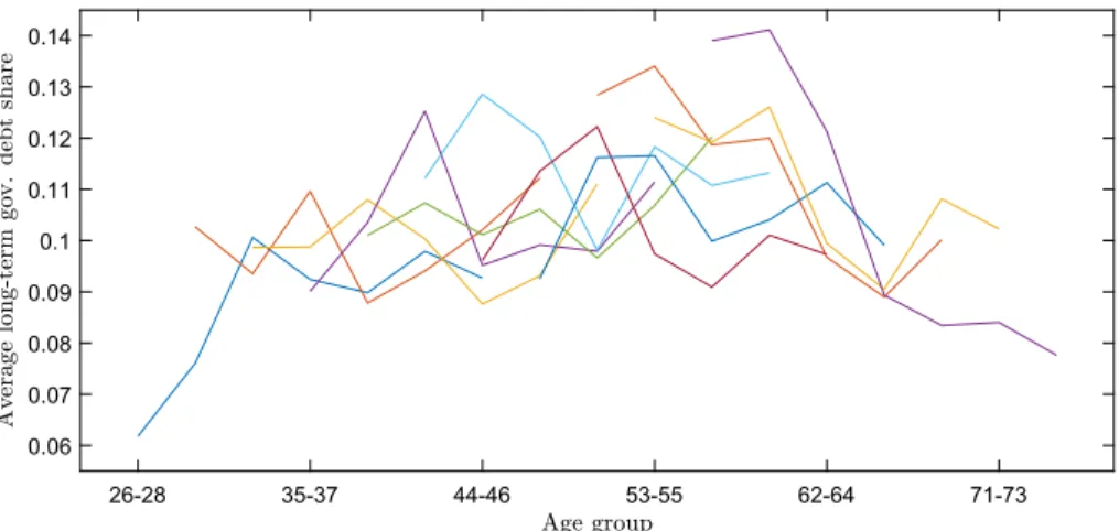
Figures1–3illustrate the average shares of the portfolio categories constructed in this way. Each line represents the average portfolio share of a given birth-year cohort at a particular age. Since data points are available only every3years, both respondent age and cohort (birth year) are divided into3-year intervals. For example, the earliest data available are from 1989. The youngest age group considered includes households with a “household head” aged26–28.8Individuals that are26–28of age in 1989 belong to the
7See EBRI Note “IRA Asset Allocation and Characteristics of the CDHP Population, 2005–2010” from May 2011, available atwww.ebri.org/publications/notes.
8In the SCF, the term “household” refers to a “primary economic unit,” which consists of a core couple or economically-dominant individual and other individuals that are financially interdependent with that
Figure1. Average portfolio share of long-term government debt.
Figure2. Average portfolio share of equity.
birth-year cohort 1961–63. The 1961–63 cohort is sampled seven times between 1989 and 2007. Its members are aged29–31in 1992, 32–34in 1995 and so on. In Figures1– 3, the lines most to the left represent the average portfolio shares held by the 1961–63 cohort. Similarly, the lines starting with age group29–31represent the average portfolio shares of the 1958–60 cohort. Altogether, the sample contains the eleven cohorts born between 1931–33 and 1961–63, each observed at seven consecutive age groups between the ages of26–28and74–76.9
The average portfolio share of stocks is increasing in household portfolios with a peak in the late fifties or early sixties of the household head. Average long-term govern-ment debt holdings behave in a somewhat similar way, although the pattern is less well pronounced. The average portfolio share of the residual category follows a pattern that is markedly distinct from that of the average long-term government bond share. However, it is a well-known fact the averages computed in Figures1–3provide a biased picture of the composition of household portfolios. The reasons are twofold.
First, the adjustments visible in the figures can be due to changes at the intensive or extensive margin. A number of papers report that the rate of participation in the stock market first increases and later decreases significantly over the life cycle.10This suggests that the inverse U-shape in Figure2largely results from households entering and exiting the stock market rather than adjustments at the intensive margin. An important ques-tion explored below is whether or not the same is true for holdings of long-term govern-ment debt. FiguresA.1toA.3, which plot the participation rates in the data, provide first suggestive evidence for the importance of adjustments at the extensive margin.
Second, as discussed inAmeriks and Zeldes(2004), it is not possible from the figures to disentangle the effects of age, observation period, and cohort. Age effects are related to education, family formation, and retirement. Period effects result from events that occur at the time of data collection. For example, the dot-com-bubble and its bursting is reflected in the survey waves from 2001 and 2004. Cohort effects include cohort-specific experiences like growing up during war time as was the case for the oldest cohorts in the sample. Even if, for example, we were to observe a figure of the same kind as Figures1– 3in which all lines were perfectly aligned such that they formed one single upward-sloping line, we could not say whether this was due to pure age effects or a combination of time and cohort effects.11
couple or individual. The “household head” is defined as the single economically-dominant individual in a household without a core couple, the male in a household with a mixed-sex core couple and the older individual in the case of a same-sex core couple.
9Only cohorts that fall inside this age interval at all seven survey waves are considered. Younger and older age groups are not examined due to a lack of sufficient data. TableA.2in theAppendixshows the number of observations for each cohort-age pair. The data set contains multiple imputations as is explained in more detail in the table notes.
10SeeAmeriks and Zeldes(2004),Fagereng, Gottlieb, and Guiso(2017), andGuiso, Haliassos, and Jappelli (2003).Haliassos(2008) contained a more general summary of the literature on limited participation in asset markets.
11Time effects could cause each individual line to be sloped upwards and cohort effects of increasing size could result in all lines aligning precisely in the way previously mentioned.
2.2 Identification
As outlined above, identification problems arise from sample selection and perfect mul-ticollinearity of a respondent’s cohort, the age at which they are sampled and the year in which the survey is conducted (birth year+age=observation period). An unresolved issue in the literature on equity holdings over the life cycle is that estimation results are somewhat dependent on the underlying identifying assumptions.12I therefore present the results obtained under three different identification strategies. Two are borrowed from the literature and one is novel. A number of robust findings emerge. To be able to motivate the strategies employed below, the nature of the identification problem is laid out before in detail.
2.2.1 Sample selection The self-selection of agents into participants and nonpartici-pants in the market for a given financial asset results in a sample selection problem. If agents enter and exit systematically over the course of the life cycle, the age effects on the conditional portfolio share are estimated with bias. To address this issue, I employ a standard latent variable model with a Probit selection equation. Formally, the model is given by
si=x2iβ2+σ12λ
x1iβˆ1+e2i (1)
∀iwheresi>0isi’s portfolio share of the asset in question,λ≡φ(x1iβˆ1)/(x1iβˆ1)is
the Inverse Mills Ratio andβˆ1is obtained from estimating the first-stage Probit model
Pr(Pi=1|x1i)=Pr x1iβ1+e1i>0 =x1iβ1 (2)
Pi=1ifiis a participant in the market for the asset considered andPi=0otherwise.
The error terms are normal,e1i∼N(01)ande2i∼N(0 σ2), withCov(e1i e2i)=σ12.
2.2.2 The “age-period-cohort problem” Due to the multicollinearity described above, a simple linear model that aims to separate age, period, and cohort effects is underidenti-fied. To see this, consider the following example.13Letaidenote the age of respondents,
ti the time period in which they are sampled andci their year of birth. Suppose that
observations are available for two consecutive time periods,ti∈ {t1 t2}, and that three
consecutive cohorts are sampled in both periods,ci∈ {c1 c2 c3}. Age can then take on
four distinct values,ai∈ {a1 a2 a3 a4}.14
A projection of some variable of interestyion age, period and cohort indicators is
yi=α1a1i +α2ai2+α3a3i+α4a4i
+θ2ti2
+γ2c2i +γ3ci3+ei (3)
12SeeAmeriks and Zeldes(2004) andGomes and Michaelides(2005) for detailed discussions. 13See alsoBrowning, Crawford, and Knoef(2012).
wherexni =1ifxi=xnandxni =0otherwise forx∈ {a t c}andn∈ {1234}. Note that
ti1, ci1 and a constant have been omitted to prevent each set of binary variables from summing to the constant. However, the fact that there exists a linear relationship be-tween the age, observation period and cohort of each respondent implies that the data matrix pertaining to equation (3) is not invertible and that parameter estimates cannot be computed using standard methods. More precisely, the linear relationship between age, period, and cohort implies15
2a1i +a2i −a4i+t2i =c2i +2ci3 (4) Inserting (4) into (3) yields
yi= ˜α1a1i + ˜α2ai2+ ˜α3a3i+ ˜α4a4i + ˜γ2c2i + ˜γ3ci3+ei (5) where ⎛ ⎜ ⎜ ⎜ ⎜ ⎜ ⎜ ⎜ ⎝ ˜ α1 ˜ α2 ˜ α3 ˜ α4 ˜ γ2 ˜ γ3 ⎞ ⎟ ⎟ ⎟ ⎟ ⎟ ⎟ ⎟ ⎠ = ⎡ ⎢ ⎢ ⎢ ⎢ ⎢ ⎢ ⎢ ⎣ 1 0 0 0 −2 0 0 0 1 0 0 −1 0 0 0 0 1 0 0 0 0 0 0 0 1 1 0 0 0 0 0 0 1 1 0 0 0 0 0 2 0 1 ⎤ ⎥ ⎥ ⎥ ⎥ ⎥ ⎥ ⎥ ⎦ ⎛ ⎜ ⎜ ⎜ ⎜ ⎜ ⎜ ⎜ ⎜ ⎜ ⎝ α1 α2 α3 α4 θ2 γ2 γ3 ⎞ ⎟ ⎟ ⎟ ⎟ ⎟ ⎟ ⎟ ⎟ ⎟ ⎠ (6)
Using equation (5), one can estimate the six reduced form parametersα˜1, α˜2, α˜3,α˜4,
˜
γ2,γ˜3. From (6), it is clear though that it is not possible to solve for the seven structural
parametersα1,α2,α3,α4,θ2,γ2,γ3knowing the reduced form parameters. The structural
parameters are underidentified, unless at least one parameter restriction is imposed. It can be easily shown that this result generalizes to scenarios with more observation periods and cohorts.
To be able to judge the robustness of the estimation results, I pursue three distinct identification strategies. The first and most standard is to impose an equality restriction on neighboring cohort effects, that is, to impose
γn=γn+1 (7)
for somen. This restriction formally reduces the generality of the model, yet the bias it introduces should be expected to be small if two neighboring cohorts can be identified that have a sufficiently similar history.
The second strategy was suggested byDeaton and Paxson(1994), and more recently used byFagereng, Gottlieb, and Guiso(2017) among others. The idea is to attribute cycli-cal fluctuations to time effects and trends to age and cohort effects. This is achieved by
15Continuing the previous example, a person that is born say in 1952 and surveyed in 2001 is aged49 when surveyed; thust2
i =ci3=a2i=1anda1i =a4i=ci2=0. It is straightforward to verify that (4) holds for all six such combinations of binary-variable values for which the birth year and the age sum to the observation period.
requiring time effects to sum to zero and to be orthogonal to a linear time trend, that is,
gθ=0 (8)
whereg=(01 T−1)is the trend,θis the vector of coefficients on the time dum-mies andTis the number of observation periods. This set of restrictions correctly identi-fies all effects if indeed only age and cohort effects are trending. In the context here, one cannot be sure however that there is no trend in time effects. In particular, in the time period examined (1989–2007), stocks became a more widely-used mode of saving. Im-posing (8) when a trend in time effects is present in the data could cause the coefficients on the age and cohort variables to jointly pick up this trend and, therefore, to be biased. In the second-stage regression, I therefore followFagereng, Gottlieb, and Guiso(2017) in detrending the dependent variable, the portfolio share of a given asset, by subtract-ing its cross-sectional average at each time period. Since this is not feasible in a binary dependent variable model, I add a linear time trend as an explanatory variable at the first stage. This implies that one additional dummy has to be excluded from the Probit model.
Under the final identification strategy, the time dummies are replaced with the first
pprincipal components of a large set of stationary macroeconomic time series covering the entire sample period. This resolves the linear dependence of the independent vari-ables. As before, the asset share is detrended and a trend is added to the selection equa-tion. To the extent that the principal components contain the effects otherwise picked up by the time dummies, this modification allows controlling for age, period, and co-hort effects without parameter restrictions. In particular, institutional and regulatory changes concerning the usage of different savings instruments can be expected to be reflected in asset prices and interest rates. Note that to provide a meaningful addition to the previous identification approach,pshould not be chosen too large.16
2.3 Estimation and results
Beginning with the second-stage regression, the equations estimated in case of the first identification strategy (parameter restriction on cohort effects) are
si=aiα2+tiθ2+ciγ2+ςλi+z2iδ2+e2i (9) Pr(Pi=1|x1i)= aiα1+tiθ1+ciγ1+z1iδ1 (10)
ai=(a26i −28 ai29−31 a74i −76) is a complete set of age dummies for seventeen age
groups, ti =(ti1992 ti1995 ti2007) is a vector of 6 year dummies and ci=(c1934i −36
16Suppose a model with Deaton–Paxson restrictions containsTtime dummies, which, together with the
two constraints that the time effects be orthogonal to a linear trend and sum to zero, can be summarized by T−2variables constructed in an appropriate way. Then, if the principal components included under the final identification strategy are also approximately orthogonal to a linear trend and mean zero, a model with p≥T−2principal components spans the same space as the one with time dummies and Deaton–Paxson restrictions. To avoid this case, it is ensured in the estimation below thatp < T−2.
Figure4. Predicted participation probabilities and conditional asset shares.
c1937i −39 ci1961−63)contains a dummy for each of ten cohorts.z2iandz1iare
addi-tional household-specific controls andx1i≡(ai ti ci z1i). In the case of the other two
strategies, the equations are modified as explained in the previous section. Information on the controls used in the estimation and a detailed discussion of the exclusion restric-tions imposed in the second step of the selection model are contained in SectionDof theAppendix.
Figure 4plots the estimation results for all three identification strategies outlined before including separate sets of results for two different cohort restrictions. The first cohort restriction equates the effects of the two oldest cohorts in the sample, 1934–36 and 1937–39, the second one those from the first two post-war cohorts, 1946–48 and 1949–51. The cohort effects of the oldest respondents are equated, since it seems likely for any differences between them to wash out over the years until the sampling period and the second restriction may appear reasonable from a historical perspective. In the model in which the time dummies are dropped, the firstp=3principal components of a large set of macroeconomic aggregates from the US are used.17Panels (a) and (c) show the marginal values, the average predicted probabilities, of being a stockholder and a long-term government debt holder, respectively, for each age group. Panels (b) and (d) graph the corresponding average predicted portfolio shares conditional on participation in the respective asset market. Since the dependent variable in (b) and (d) is detrended
17Details about the macroeconomic time series employed and the principal components are given in the Online Appendix found in the Supplementary Material of this paper (Tischbirek(2019)) of this paper.
when the Deaton–Paxson restrictions are imposed and when the principal components are used to capture time effects, the mean asset share conditional on participation is added to the average predicted values in these two instances to produce the estimates shown.
From the figure, it becomes obvious that imposing different ex ante plausible co-hort restrictions does not yield robust estimates. While all estimates for long-term debt market participation are of similar shape, the estimates obtained when cohort restric-tions are employed deviate significantly from each other and from the results obtained under the remaining two identification schemes in the panels (b) to (d). Experimenting with different cohort restrictions showed that the discrepancies are even more severe for other pairs of economically plausible restrictions, likely because trends in the cohort effects not accounted for by the model are forced into the estimates of the age effects. However, the results obtained using Deaton–Paxson restrictions and principal compo-nents nearly coincide despite of their distinct way of accounting for time influences and are consistent with previous findings about equity holdings from the literature.18
Several stylized facts emerge from the estimations that make use of Deaton–Paxson restrictions or principal components. The profile of participation in the market for long-term government debt shows a pronounced hump shape. Participation rates rise over the course of nearly the entire working life and then begin to decline at the age of62– 64as household members retire. The age effects on the conditional portfolio share of long-term government debt are mildly increasing at first and roughly constant from the mid-forties until retirement. A significant decline is not observable until after the age of65. Overall, the results suggest that there is a clear inverse U-shape in participation rates and that the conditional portfolio share is nondecreasing until retirement, but falls thereafter. Stock market participation takes an almost identical shape to participation in the market for long-term government debt. The conditional stock share is monotone declining from39–41onwards.
The life-cycle dynamics of stock-market participation and the conditional share of stocks have been a topic of debate in the literature. In summarizing the existing empir-ical evidence,Gomes and Michaelides(2005) stated that (1) stock-market participation increases over the working life, (2) there is some evidence which suggests that participa-tion rates decline after retirement, and (3) there is “no clear pattern of equity holdings over the life cycle.” I interpret the results presented here as support for (1) and (2). In re-cent work,Fagereng, Gottlieb, and Guiso(2017) found evidence for the conditional stock share to decline over the life cycle using administrative panel data from the Norwegian Tax Registry.19Regarding (3), my estimates are more in line with their findings.20
Table2provides more detailed information about the estimations for the long-term debt share. The results from the models with cohort restrictions are included for
com-18The estimated cohort and time effects are shown in the Online Appendix.
19Considering cross-sectional data only, other studies conclude that the conditional equity share may be mildly increasing or also mildly hump-shaped; seeCampanale, Fugazza, and Gomes(2015) for a short discussion.
20In the Online Appendix, it is shown that the stylized facts are robust to reassigning corporate bond holdings to the long-term debt category.
Table2. Estimation results for long-term government debt share.
Deaton–Paxson Principal Comp. Cohort Restr.1 Cohort Restr.2 1st st. 2nd st. 1st st. 2nd st. 1st st. 2nd st. 1st st. 2nd st. λ 0065 0066 0065 0065 (0021) (0021) (0021) (0021) ρ 0445 0449 0445 0445 min(Nimp) 17,202 12,673 17,202 12,673 17,202 12,673 17,202 12,673 TotalN 86,030 63,437 86,030 63,437 86,030 63,437 86,030 63,437 Sign. tests Age eff’s 0000 0066 0000 0090 0000 0000 0000 0000 (d.o.f.) (16) (17) (16) (17) (17) (17) (17) (17) Time eff’s 0029 0325 0051 0000 0051 0000 (d.o.f.) (5) (5) (6) (6) (6) (6) Cohort eff’s 0319 0007 0318 0094 0256 0114 0256 0114 (d.o.f.) (10) (10) (10) (10) (9) (9) (9) (9) Pri. comp’s 0027 0153 (d.o.f.) (3) (3)
Note: Results of first and second stage estimation shown for four models—Deaton–Paxson restrictions, principal compo-nents of macroeconomic variables replacing time dummies, cohort effects equated for ’34–’36and ’37–’39(Cohort Restr.1), cohort effects equated for ’46–’48and ’49–’51(Cohort Restr.2). Models estimated using two-step estimator (Heckit). Data are multiply imputed. For each respondent, there are five observations in the data. Point estimates are averages over five sep-arate estimations. Strd. errors (in parentheses) are adjusted in an appropriate way.Nimpis number of obs. for imputation imp∈ {12 5}. For joint significant tests, avrg. p-value shown (each test stat.∼χ2), degrees of freedom in parentheses.
parison purposes. The coefficient on the inverse Mills ratioλis significant and the corre-lation of first-stage and second-stage residualsρis estimated to be positive, confirming the need to address the selection problem. SCF data are multiply imputed. The size of the smallest imputation groupmin(Nimp)therefore gives a more accurate picture of the
number of respondents in the sample than the total amount of observationsN. With Deaton–Paxson restrictions and principal components, all age effects are significant. The significance level is slightly higher in the selection equations than in the conditional portfolio share equations, in line with the estimated size of the slope coefficients. Time effects play an important role at the first stage but cease to do so at the second stage. Thus, the participation decision is strongly influenced by time effects even after con-trolling for a linear trend. Demeaning the conditional long-term debt share successfully eliminates time effects at the second stage. The estimated cohort effects are jointly sig-nificant only for the conditional asset share.
To uncover the interdependence between the different portfolio components, I addi-tionally estimate the models for the stock share with (financial and nonfinancial) wealth and either the long-term bond share or the share of the residual category “cash” as in-dependent variables. The results are shown in Table3. Conditional on wealth, a higher long-term debt share is correlated with a higher probability of being a stockholder, while the opposite is true for the portfolio share of cash, as one would expect. The estimates from the second stage suggest that the elasticities of substitution between long-term debt and equity and between cash and equity differ, reflected in coefficients of−052
Table3. Substitution of long-term government debt and cash with equity.
Deaton–Paxson Deaton–Paxson Principal Comp. Principal Comp. 1st st. 2nd st. 1st st. 2nd st. 1st st. 2nd st. 1st st. 2nd st. Long-t. debt 3305 −0516 3306 −0516 (0164) (0022) (0164) (0022) Cash −5241 −0884 −5239 −0884 (0119) (0008) (0119) (0008) Wealth 00066 00004 00041 00000 00066 00004 00041 00000 (in millions) (00013) (00001) (00013) (00000) (00013) (00001) (00013) (00000) min(Nimp) 17,202 12,750 17,202 12,750 17,202 12,750 17,202 12,750 TotalN 86,030 63,799 86,030 63,799 86,030 63,799 86,030 63,799 Sign. tests Age eff’s 0000 0000 0000 0000 0000 0000 0000 0001 (d.o.f.) (16) (17) (16) (17) (16) (17) (16) (17) Time eff’s 0000 0096 0000 0033 (d.o.f.) (5) (5) (5) (5) Cohort eff’s 0332 0000 0231 0041 0234 0000 0465 0241 (d.o.f.) (10) (10) (10) (10) (10) (10) (10) (10) Pri. comp’s 0000 0027 0000 0019 (d.o.f.) (3) (3) (3) (3)
Note: Results of first and second stage shown for four models estimated using two-step estimator (Heckit). Data are multiply imputed. For each respondent, there are five observations in the data. Point estimates are averages over five sep-arate estimations. Strd. errors (in parentheses) are adjusted in an appropriate way.Nimpis number of obs. for imputation imp∈ {12 5}. For joint significant tests, avrg. p-value shown (each test stat.∼χ2), degrees of freedom in parentheses.
and−088, respectively.21Additional cash holdings are associated with a larger reduc-tion in the stock share than addireduc-tional long-term debt holdings. In addireduc-tion to differing age profiles, this suggests that long-term debt plays a significant and distinctive role in the dynamic rebalancing of household portfolios. The model outlined in the following section allows studying these relationships in more detail.
3. Model
There is a large number of agents who are faced with an asset market participation de-cision and, conditional on participation, an asset allocation problem in each period of their lives. I refer to model agents interchangeably as households or investors below.22 Investors are born employed. They retire and subsequently die, providing them with a motive to save for retirement and to deplete their asset stock once retired. Asset market participation is costly, but allows an investor to hold stocksandlong-term government debt. A non-participant is able to save only through a riskless and low-interest bearing
21Significantly differing values also emerge from a naive OLS regression among stock and long-term debt holders. See TableA.3in theAppendix.
22A model agent can be viewed as a household that either is in direct control of the consumption-savings and the portfolio-choice decision or delegates the latter decision to a portfolio manager that is informed about the risks faced by the household and its preferences toward them.
asset that is comparable to short-term bonds or cash. Thus, agents who choose to invest in only one of the two risky assets have to incur the entire asset market participation cost.23 Investors are subject to uninsurable idiosyncratic and aggregate risk. Idiosyn-cratic risk arises from nonfinancial income and aggregate risk results from the returns on stocks and long-term government debt.
3.1 Life-cycle stages
Each investori∈Ilives forTperiods and goes through an employment and a retirement stage. Investors are born employed at the beginning of periodt=1, retire in periodTret>
1and die at the end of periodT > Tret. Note that the model describes the decisions of a
large number of agents belonging to thesamegeneration and that, as a result, there is no interaction between different, potentially overlapping, generations. Investors supply labor inelastically as long as they remain employed, which entitles them to an exogenous income stream given by
Yit=PitUit lnUit∼N −05σu2 σu2 (11) Pit=GPit−1Nit lnNit∼N −05σn2 σn2 (12)
Labor income has a transitory componentUit and a persistent componentPit.24 The
logarithm ofPit follows a random walk with drift. The expectation of the shock to the
persistent component of income Nit and the expectation of the transitory shockUit
equal one, so that, in expectation, the labor income of all agents grows at the common rateG−1.25Retired investors receive a pensionΩ
it=ωPiTretwhich is a fraction of the
persistent income that they obtained in the last period in which they were employed as in the model ofGomes and Michaelides(2005) among others. This specification cap-tures the empirical fact that differences in income that develop over the course of the working life persist among retired investors.
3.2 Investment opportunities
There are three types of assets available to the investors: a one-period bond, stocks, and long-term government debt. Long-term government debt has a maturity ofδperiods. A strategy frequently adopted in the literature is to assume that long-term bonds are en-tirely illiquid, or more precisely, that they have to be held until maturity. Aside from un-derstating the liquidity of long-term government debt, this assumption leads to a big in-flation of the state space asδbecomes large, causing exact solutions to portfolio choice
23The model does not include separate participation costs for the long-term government debt market and the stock market to reduce the dimensionality of the portfolio choice problem. Participation in both markets is highly correlated in the sample with a coefficient of080and Figure4suggests that this simplifi-cation yields a good approximation of observed household behavior. FigureA.8shows that reestimating the empirical models with a joint asset-market participation decision does not alter the stylized facts described in the previous section.
24This income process is frequently used in the literature and originally due toCarroll, Hall, and Zeldes (1992). They refer toPsomewhat ambiguously as “permanent labor income.”
problems to be computationally burdensome. A specification is proposed here that, in accordance with the US long-term bond market, allows investors to access some of the funds held in the form of long-term debt in each period and that makes the portfolio optimization computationally feasible.
An investor that has purchased long-term government bonds in periodt−1at the amount ofQit−1receives a Calvo-type signal for each infinitesimal unit ofrqtQit−1in
periodtindicating whether it can be sold or not.rqt is the annual gross return on the
long-term government bond. A positive signal is received with probabilityδ−1, implying that each infinitesimal unit has to be held on average forδperiods. Thus, portfolios are chosen in all periods subject to the constraint
Qit≥
1−δ−1rqtQit−1 (13)
Comparable to the case in which long-term bonds have to be held until maturity, the minimum expected holding period of the entire stock is equal to its maturity, but a frac-tion of this stock can be accessed in each period. Since the probability of being able to sell a given unit of long-term debt is time-constant, all long-term debt held byican be summarized by one single state variable. Modeling long-term government bonds as a perpetuity as inWoodford(2001) would equally permit all long-term debt to be repre-sented by a single state variable. However, the specification chosen here emphasizes the imperfect liquidity of long-term government debt, which is an important characteristic of assets such as US savings bonds and tax-exempt bonds.26
The one-period bond yields the riskless gross return rb. Following Bonaparte,
Cooper, and Zhu (2012), the gross stock return rst evolves according to a two-state
Markov process,rst∈ {rsl rsh}, with meanrs and standard deviationσrs. Accounting for
capital gains and dividends,Bonaparte, Cooper, and Zhucannot reject that the annual stock return in the US is serially uncorrelated.rstis therefore assumed to be i.i.d. across
periods with probabilities of a half for both return states. The return on long-term gov-ernment debt equally follows a two-state Markov process. The mean, the standard devi-ation, and the transition matrix are given byrq,σrq, andrq, respectively. No restrictions
are placed onrq, allowing for persistence in the government bond return process.
Holdings of the short-term bondBitare costless. Investments in stocksSitand
long-term government debtQitare associated with a cost of sizeΨit=ψPitifiis employed
andΨit=ψPiTret if iis retired that has to be paid in each period of active
participa-tion in the markets for stocks or long-term government debt.Ψitrepresents, for
exam-ple, costs associated with the acquisition of information about financial markets and is scaled to the persistent component of income in order to capture the opportunity cost of time.27 Investors are not considered active participants in financial markets if they hold no stocks and allow potential previously-acquired holdings of long-term bonds to
26The two specifications are similar though. For a perpetuity, the pay-off stream from a one-dollar in-vestment isρ ρ2 ρ3 for someρ∈ [0 β−1). Here, if government debt is run down at the fastest possible rate, this stream is(1−δ−1)rqt+1 (1−δ−1)2rqt+1rqt+2 (1−δ−1)3rqt+1rqt+2rqt+3 with(1−δ−1)∈ [01).
27InAlan(2006), the cost of stock-market participation is equally made dependent on the persistent component of labor income, however, it is incurred only the first time an agent enters the market and not, for example, at a later reentry.
mature at the fastest possible rate. Thus, if the investor chooses not to payΨit,Sit=0
and (13) holds with equality.28In addition, stock holdings are subject to a variable cost
ψsSit, reflecting the monetary costs of maintaining a stock portfolio. The role played by
the two types of costs is revisited below in more detail. 3.3 Optimization problem
The optimal plan of investori∈Isolves the problem described in this section in each periodt=12 T. The indicesiandtare suppressed below for notational clarity. 3.3.1 Financial-market participants The budget constraint of an investor that partici-pates in financial markets is given by
C+S(1+ψs)+B+Q+Ψ=rsS−1+rbB−1+rqQ−1+Θ (14)
where nonfinancial incomeΘ∈ {Y Ω}equalsY if the investor is employed andΩ oth-erwise. The sum of expenditures on consumption, stocks, short-term bonds, long-term government debt, and all costs incurred must be equal to income, which is given by the gross return on last period’s investments and nonfinancial income.
Defining “cash on hand” as
X≡rsS−1+rbB−1+δ−1rqQ−1+Θ (15)
and illiquid assets as
Z≡1−δ−1rqQ−1 (16)
one can express the budget constraint as
C+S(1+ψs)+B+Q+Ψ =X+Z (17)
In equation (17), income is divided into liquid fundsX that can be freely allocated to-ward all types of expenditures and illiquid fundsZwhich are tied to a reinvestment in long-term government debt. Using this notation, the liquidity constraint on long-term government (13) debt becomes
Q≥Z (18)
requiring investors to carry an amount of long-term debt forward into the next period that is at least as large as the amount of illiquid assets brought into the period.
In the event of participation in the current period, the optimal portfolio choice sat-isfies
vp(X Z rq P t)= max
CSBQu(C)+βEUPrsrq|Prqv
X Z rq P t+1 (19)
28If nonparticipants were able to reduce long-term bond holdings at a faster rate, there would be liq-uidity gains associated with not acquiring information about financial markets. If they were able to reduce long-term bond holdings at a slower rate, the expected average holding period of long-term bonds would be larger than the maturity of the bond. Therefore, the assumption that (13) must hold with equality for nonparticipants seems most plausible.
together with (15)–(18) and the regularity conditions (S B Q)≥(S B Q). Here, u:
R+ →R is the period utility function with u(C) >0and u(C) <0 for all C ∈R+,
vp:R2×(R+)2×N→Ris the indirect utility function conditional on financial-market
participation in the current period andvis unconditional indirect utility derived below. Since retirement income is deterministic, the expectation has to be taken overUandP
only if the investor is employed.
3.3.2 Financial-market nonparticipants The budget constraint of a household that does not participate in financial markets is
C+B+Q=rsS−1+rbB−1+rqQ−1+Θ
=X+Z (20)
As discussed before, for a nonparticipant
Q=Z (21)
which implies that the budget constraint can be written as
C+B=X (22)
The equation above is independent ofQ, reflecting the fact that the only choice that a nonparticipant faces is how to allocate cash on hand toward consumption and savings at the risk-free rate.
In this case, the solution must satisfy
vn(X Z rq P t)=max
CBu(C)+βEUPrq|Prqv
X Z rq P t+1 (23) as well as (15), (16), (20), (21), andB≥B, wherevn:R2×(R+)2×N→Rgives indirect
utility if the household does not participate and retired agents face no risk from nonfi-nancial income as explained above.
3.3.3 Participation decision In each period, an investor has to decide whether or not to participate in financial markets having solved the consumption-savings problem and the portfolio choice problem in the case of participation. The value of the problem of an investor is given by v(X Z rq P t)=max vp(X Z rq P t) vn(X Z rq P t) (24)
At each point in the state space, the investor decides to participate in financial markets if the value from participating is higher than that from not participating.
3.4 Computation
The model has to be solved numerically. The fact that agents are able to invest in a third financial asset with a persistent stochastic return increases the dimensionality of the problem significantly in comparison to other recent models of portfolio choice over the
life cycle.29There are three continuous state variables in addition to the prevailing level of the return on long-term debt and the investors’ age. The optimization involves four continuous controls. One state variable can be eliminated from the problem by divid-ing all endogenous variables by the persistent component of labor income P. Below, lower case letters denote normalised variables, for example,x≡X/P. Period utility is assumed to be of CRRA form with a coefficient of relative risk aversionγ. This implies that all value functions introduced above are homogeneous of degree1−γ. For exam-ple, the indirect utility of an employed investor that participates in financial markets in the current period can be expressed as
vp(x z rq t)= max csbqu(c)+βEUNr qrs|rq GN1−γvx z rq t+1 (25) The stochastic growth rate of the persistent component of incomeP/P=GN raised to1−γ now premultipliesv in the expected value accounting for uncertainty result-ing from persistent income shocks. All normalized model equations together with more details on their derivation are listed in SectionEof theAppendix.
3.5 Calibration
Table4shows the calibration used for the simulations presented in the sections that follow. Note that the model is written entirely in real terms. A period corresponds to a year. Since the age group26–28is the youngest contained in the estimations described in Section2, it is assumed that agents are born at the age of27.TretandT are selected
such that agents retire just before turning63years of age and die at the age of80, respec-tively, consistent with data from the US Census Bureau. A value of five forδimplies that the long-term bond approximates5-year government debt. This is in line with the aver-age maturity of all outstanding marketable securities issued by the US Treasury which averaged597months between January 2000 and December 2007.30
As in Bonaparte, Cooper, and Zhu (2012) and Campanale, Fugazza, and Gomes (2015), the risk-free rate is set to 2%, a value that is commonly used in the literature. Bonaparte, Cooper, and Zhufurther estimated the average net return of stocks in the US, inclusive of dividend payments, to be633%with a a standard deviation of0155and no serial correlation, which I also adopt here. The mean excess return of5-year govern-ment debt over the risk-free rate is set to06%, the standard deviation of5-year US debt over the sampling period was about0011. The5-year government debt return is mod-eled using a two-state Markov process whose transition matrix is found by first fitting an AR(1)process to the data and then finding the transition probabilities that best describe the estimatedAR(1)process as proposed inTauchen and Hussey(1991).rqremains in
statek∈ {l h}with probability0663and switches with the converse probability.
The standard deviations of the shocks to the transitory and the persistent compo-nent of income are chosen based on the estimates reported in the seminal contribu-tion byCarroll, Hall, and Zeldes(1992). Several papers draw on these results, including
29Examples of models with two assets includeBonaparte, Cooper, and Zhu(2012),Campanale, Fugazza,
and Gomes(2015), andCocco, Gomes, and Maenhout(2005).
Table4. Calibration.
Parameter Value Description Target/Source
Tret 36 Retirement period Avrg. US retirement age
T 54 Death period US life expectancy
δ 5 Maturity of government debt Avrg. maturity of marketable US debt
β 096 Discount factor Gomes and Michaelides (2005)
γ 5 Coefficient of relative risk aversion Gomes and Michaelides (2005) σu 016 SD of log transitory income shock Carroll, Hall, and Zeldes (1992) σn 012 SD of log persistent income shock Carroll, Hall, and Zeldes (1992)
G 103 Mean income growth Haliassos and Michaelides (2003), Viceira (2001)
ω 06 Replacement ratio Campanale, Fugazza, and Gomes (2015),
Munnell and Soto (2005)
rb 102 Gross return of riskless bond Bonaparte, Cooper, and Zhu (2012) rs 10633 Mean gross stock return Bonaparte, Cooper, and Zhu (2012) σrs 0155 SD of stock return Bonaparte, Cooper, and Zhu (2012) rq 1026 Mean gross return ofδ-year bond 5-year Treasury Notes return σrq 0011 SD ofδ-year bond return 5-year Treasury Notes return rqkk 0663 Pr(rqk|rkq)fork∈ {l h} 5-year Treasury Notes return ψs 0015 Variable cost of stock holdings Avrg. expense ratio of equity funds ψ 0035 Participation cost parameter Campanale, Fugazza, and Gomes (2015),
Gomes and Michaelides (2005)
B,Q,S 0 Borrowing limits Campanale, Fugazza, and Gomes (2015)
Gomes and Michaelides(2005) andHaliassos and Michaelides(2003).Carroll, Hall, and Zeldes(1992) set income growth to2%, subsequent papers use a slightly higher value of 3%, which I follow here (Haliassos and Michaelides(2003),Viceira(2001)). The re-placement ratio employed is 06in line withCampanale, Fugazza, and Gomes(2015) andMunnell and Soto(2005).31
A number of authors that examine stock holdings over the life-cycle report estimates of the discount factor and the coefficient of relative risk aversion. Although the results vary considerably, generally a relatively high degree of discounting and risk aversion is required to match the data. The estimates ofBonaparte, Cooper, and Zhu (2012) are
β=069andγ=724.Alan(2006) estimatedβ=092andγ=16.Cagetti(2003) showed that both variables strongly depend on education with estimates for groups of differ-ent education levels ranging from078to114forβand from240to813forγ. Cam-panale, Fugazza, and Gomes(2015) employedβ=094andγ=5. FollowingGomes and Michaelides(2005), I use standard values ofβ=096andγ=5.32
31Munnell and Soto(2005) found that, in the US, the replacement rate ranges from about06to08for households covered by a pension plan and from about045to06for those without pension coverage de-pending on the precise definitions used.
32As inAlan(2006) andBonaparte, Cooper, and Zhu(2012), expected utility is discounted at a constant rate. Time-variation in the discount factor could be introduced through age-dependent conditional death probabilities which according to data from the National Center for Health Statistics (NCHS) are small until old age though.
The high structural estimates for the discount rate and the coefficient of relative risk aversion are related to a puzzle that poses a challenge to the literature on portfo-lio choice over the life cycle. According to standard models, it is optimal for households to invest a bigger share into high-risk and high-return assets like stocks than they do according to survey data. A number of strategies have been employed to align model-based predictions more closely with the empirical evidence. Calibrations with high, oc-casionally extreme levels of discounting and risk aversion respectively lower the ben-efits from the high average return and increase the sensitivity of households toward the high volatility of stocks. Transaction costs which imply that investors cannot cost-lessly convert stock holdings into consumption equally reduce the value of stock hold-ings for households (Campanale, Fugazza, and Gomes(2015)). Disastrous labor income shocks occurring with a small probability make total income, ceteris paribus, more risky and, therefore, lead households to reduce portfolio risk by lowering the stock share. Fi-nally, an isolated decrease in the elasticity of intertemporal substitution, implemented by generalizing CRRA utility to the Epstein–Zin–Weil recursive form, causes households to increase savings, and thus financial income which also implies a lower optimal stock share.33
The focus of this paper lies on the dynamic patterns according to which liquidity, long-term debt, and stocks are substituted as wealth is accumulated and deaccumu-lated with age rather than the effect that the addition of long-term debt to the portfo-lio choice problem of households has on the mean level of stock holdings. To keep the analysis as clean as possible, therefore merely two types of realistically-calibrated costs whose effects are easily understood are included in the model. The fixed cost of asset-market participationψgives rise to a meaningful participation decision and the variable cost of stock holdingsψsto an interior solution to the conditional asset allocation
prob-lem.Gomes and Michaelides(2005) calibrated stock-market entry costs to25%of the persistent component of labor income,Alan(2006) estimates a value of about21%. In the model ofBonaparte, Cooper, and Zhu(2012), agents incur a transaction cost in each period in which stock holdings are adjusted. Their estimate for these costs is12%of total labor income.Campanale, Fugazza, and Gomes(2015) consider transaction costs that are comparable to those inBonaparte, Cooper, and Zhu(2012) which they calibrate to4%–7%, depending on the level of education, in a their preferred scenario. In accor-dance with these values,ψis set to35%here.
The Investment Company Institute (ICI) publishes data on the fees associated with investments in equity funds, which I use as an approximation of the marginal cost of holding a stock portfolio. The average expense ratio, the ratio of annual fees to the total size of the investment, fell from16%in 2000 to15%in 2007 and13%in 2015.34Based on these figures, a value of15%is chosen forψs. Following the literature, the
possibil-ity of borrowing and short selling is excluded in the model (Campanale, Fugazza, and Gomes(2015)).35
33SeeCocco, Gomes, and Maenhout(2005) for more details on the effects of disastrous labor income shocks and changes in the elasticity of intertemporal substitution.
34Seewww.icifactbook.org. Asset-weighted averages are slightly smaller, however, the expense ratio does not include costs like portfolio transaction fees, brokerage costs, or sales charges.
3.6 Portfolio rebalancing
The policy functions associated with the optimisation problem laid out above illustrate how investors rebalance their portfolios as financial wealth increases. In Figure5, the
optimal choice of financial assets is plotted against cash on hand at different ages. Po-tential illiquid asset holdings brought into the period are set to zero for now. The long-term interest rate is in its low state in the panels on the left and in its high state in the panels on the right. All variables are normalized by the trending persistent component of income as described before.
The solution follows a similar pattern at all ages shown with the exception of the last. It is highly nonlinear. At very low levels of cash on hand, investors do not participate in the markets for stocks and long-term debt. All savings are done using the risk-free as-set since the higher expected returns obtainable when they participate would not suf-ficiently compensate investors for the additional risks born and the participation cost as well as the proportional costs incurred. As cash on hand increases, the benefits from participating in financial markets outweigh the costs. Holdings of the riskless asset as a savings device then play a role only for older households and younger households with significantly larger levels of cash on hand than are shown in the figure.36Note that con-sumption, given by the difference between the45-degree line and riskless bond holdings for nonparticipants, initially remains nearly constant as investors aim to accumulate wealth.
Just above the participation threshold, agents allocate their investments toward stocks. As cash on hand increases, investors reduce the risk that they are exposed to
through their financial portfolioby rebalancing their portfolios away from stocks and to-ward government debt. Because the expected return on long-term debt is higher when it is currently in the high state, investors start to substitute long-term debt for stocks at lower levels of cash on hand in this case.
To understand why portfolios are adjusted in this way, suppose first that labor and retirement income were nonstochastic. At low levels of cash on hand, labor and retire-ment income make up a large part of overall income. Thus, investretire-ments in financial as-sets could be comparably risky without giving rise to much risk exposure on aggregate. At high levels of cash on hand, labor and retirement income make up only a small frac-tion of overall income. Thus, investors would be exposed to more risk on aggregate if the same share of investments were made in the form of stocks. As a result, given that rela-tive risk aversion is assumed to be constant, an equal or even increasing portfolio share of stocks across cash-on-hand levels could not be part of the solution to the investors’ portfolio choice problem.37
Viceira(2001) showed that investors with stochastic nonfinancial income behave in an analogous way. Provided that the nonfinancial income is uncorrelated with the asset returns, agents choose their portfolios as if this income were generated by an invest-ment in a safe asset of a size below the expected discounted value of its future payinvest-ment
36There is no intrinsic value of holding the riskless asset in the model. A more significant portfolio share would be obtained for financial market participants, for example, if this asset were interpreted as “money” and a cash-in-advance constraint were introduced.
37The initial increase in the risk exposure of asset market participants at cash on hand levels beyond the “kink” in holdings of the riskless asset is a result of the lower bound on government debt and riskless bond holdings. Without borrowing constraints, investors would hold negative amounts of at least one of the two assets initially.
stream.38Consequently, they also reduce the stock share in their financial portfolio as wealth is accumulated. A comparable effect can be observed in models in which in-vestors have the choice between stock and a safe asset only.39In this class of models, it is the share of the riskless asset that increases with cash on hand as the stock share is reduced. At high levels of wealth, these models therefore assign a role to money holdings as a savings instrument that the model discussed here partly assigns to long-term debt holdings.
At the retirement stage, here represented by the policy functions of an investor at the age of70, stock holdings are smaller for all levels of cash on hand than at younger age. Lower nonfinancial earnings imply that households reduce the risk incurred through their portfolio. Because long-term debt is partially illiquid, stock holdings are substi-tuted with holdings of the safe asset toward the end of the life cycle.
The policy functions depend on the model parameters in an intuitive way. An in-creased excess return of long-term debt induces employed investors to rebalance stocks towards debt at lower levels of cash on hand. Higher participation costs defer asset mar-ket participation, particularly during the retirement phase. Less risk aversion, a smaller discount factor and a higher retirement age lead investors to enter asset markets at lower wealth levels. The corresponding figures for investors at the age of40and70are con-tained in the Online Appendix.
Figure6shows how the investment decisions are influenced by existing long-term bond positions. It plots the optimal level of investment in all three financial assets against cash on hand for increasing values of illiquid wealthz. Results are only shown for an investor aged60, that is, an employed investor who is likely to have accumulated illiquid assets, andrq=rql for conciseness. The higher the illiquid wealth of households,
the less they invest in the riskless asset conditional on not participating in government-debt and equity markets and the more liquid wealth is required to make full asset market participation worthwhile. Intuitively, the more funds are currently locked up in previ-ous investments but will become available in the future, the less willing investors are to pay the participation fee to make new investments in stock or long-term bonds. The optimal amount of new long-term bonds purchased is constant as long as the liquidity
Figure 6. Optimal holdings of the riskless asset (left), long-term debt (middle), and stocks (right) as a function of liquid and illiquid financial wealth (age60,rqin low state).
38This is shown formally in Proposition 3 ofViceira(2001).
constraint is binding. The more illiquid wealth investors possess, the higher is the level of liquid assets at which they wish to hold long-term bonds in excess of the required amount.
4. Simulations
This section reports results from simulations of the baseline model outlined above and an application to the period of historically low US Treasury returns between 2009 and 2013.
4.1 Baseline results
I simulate the model for T =80−26=54 years, forI individuals with idiosyncratic shocks{Uit Nit}Tt=1, and forJaggregate shock sequences{rst rqt}Tt=1.IandJare
cho-sen sufficiently large to guarantee full convergence of all model moments precho-sented be-low. Households have an initial endowment of liquid financial assets amounting to50% of the permanent component of labor income and half of the households additionally have illiquid initial wealth at the value of25%of permanent labor income, which is ap-proximately in line with the data from the SCF. Figure7plots the participation rate and the asset shares conditional on participation implied by the model against the empirical estimates from Section2. The estimates shown use the Deaton–Paxson identifying as-sumptions and principal components to capture time effects, respectively. The behavior of households in the SCF coincides with the predictions of the life-cycle model in several ways.
The dynamics of asset market participation in the model mirror the patterns of par-ticipation in the markets for equity and long-term debt estimated from the SCF data. Participation in financial markets is low at first in the model, since initial wealth and hence desired savings are too low for it to be profitable to pay the participation cost and then increases sharply as agents accumulate wealth. The participation rate first flat-tens and then peaks at the age of59–61. It declines again as agents retire and fall back to wealth levels at which paying the participation cost to invest in the two risky assets ceases to be beneficial.
The panels (b) and (d) show the average simulated conditional asset shares together with the corresponding empirical estimates. The conditional long-term government debt share in the model increases between the ages of35–37and 62–64and then de-clines. A comparable pattern is visible but less well pronounced in the data. The long-term debt share equally increases between32–34and41–43as well as between44–46 and 53–55but at a smaller scale and the estimated peak occurs at a slightly younger age. Because cash on hand on average increases with age during the employment stage, households rebalance their portfolios from stocks toward long-term bonds to reduce the risk they are facing through their financial portfolio in the model. Accordingly, the model predicts a declining conditional stock share over the course of the working life which is confirmed by the SCF data. When agents retire, nonfinancial income falls which implies that they wish to decrease the risk of their financial investments. The fact that agents also save less partially offsets this effect. On aggregate the stock share continues to de-cline. The lack of liquidity of long-term debt makes it increasingly less attractive as a replacement for stock holdings during the retirement phase. Since both the stock share and the long-term debt share fall, the share of the residual category increases. The em-pirical estimates suggest that the same is true in the US data.
While the stylized facts about the life-cycle dynamics of asset market participation, the conditional stock share and the conditional long-term debt share uncovered in Sec-tion2can be rationalized using the model, the predicted dynamics are more muted in the SCF estimates compared to the model. This may suggest that a standard life-cycle model somewhat overstates the responsiveness of US households to life-cycle influ-ences but may equally be a result of noise in the survey data or the fact that a part of the asset holdings have to be imputed. The investment decisions of the model agents are crucially driven by wealth accumulation. Therefore, it is instructive to investigate the evolution of wealth in more detail to further gauge the congruence of observed house-hold decisions with optimal model behavior.
Figure 8compares the distribution of wealth normalized by nonfinancial income for six intermediate age groups of employed investors in the model and in the SCF.40 In both cases, kernel density estimates based on a Gaussian kernel are reported.41The
40In the model, wealth is the sum of liquid and illiquid funds normalised by the permanent component of labor income (x+z). In the SCF data, I construct the corresponding measure by summing financial assets (financial asset holdings and income from interest and dividends) with nonfinancial income (wage income, retirement income, and transfers) and dividing by the latter.
41The distributions from the data are obtained by pooling the survey waves contained in the sample for each age group.