3
Institute of Economics
HOHENHEIM DISCUSSION PAPERS
IN BUSINESS, ECONOMICS AND SOCIAL SCIENCES
A DATA-DRIVEN PROCEDURE TO
DETERMINE THE BUNCHING WINDOW
- AN APPLICATION TO THE NETHERLANDS
Vincent Dekker
Kristina Strohmaier
Nicole Bosch
University of Hohenheim
Discussion Paper 05-2016
A Data-Driven Procedure to Determine the Bunching Window *
An Application to the Netherlands
-Vincent Dekker, Kristina Strohmaier, Nicole Bosch
Download this Discussion Paper from our homepage: https://wiso.uni-hohenheim.de/papers
ISSN 2364-2076 (Printausgabe) ISSN 2364-2084 (Internetausgabe)
Die Hohenheim Discussion Papers in Business, Economics and Social Sciences dienen der schnellen Verbreitung von Forschungsarbeiten der Fakultät Wirtschafts- und Sozialwissenschaften.
Die Beiträge liegen in alleiniger Verantwortung der Autoren und stellen nicht notwendigerweise die Meinung der Fakultät Wirtschafts- und Sozialwissenschaften dar.
Hohenheim Discussion Papers in Business, Economics and Social Sciences are intended to make results of the Faculty of Business, Economics and Social Sciences research available to the public in
order to encourage scientific discussion and suggestions for revisions. The authors are solely responsible for the contents which do not necessarily represent the opinion of the Faculty of Business,
A Data-Driven Procedure to Determine the Bunching Window
*An Application to the Netherlands
-Vincent Dekker Kristina Strohmaier† Nicole Bosch§ 13th May 2016
Abstract
This paper presents new empirical evidence on taxpayers’ responsiveness to tax-ation by estimating the compensated elasticity of taxable income with respect to the net-of-tax rate in the Netherlands. Applying the bunching approach intro-duced by Saez (2010), we find small, but clear evidence of bunching behaviour at the thresholds of the Dutch tax schedule with a precise estimated elasticity of 0.023 at the upper threshold. In line with the literature, we find much larger estimates for women and self-employed individuals, but we can also identify signi-ficant bunching behaviour for wage employed individuals which we can attribute to tax deductions for couples. We add to the bunching literature by proposing to rely on the information criteria to determine the counterfactual model, as well as developing an intuitive, data-driven procedure to determine the bunching window.
JEL Classification: H21, H24
Keywords:
Bunching, Elasticity of Taxable Income, Optimal Bunching Window
*We thank Nadja Dwenger, Nadine Riedel, Robert St¨uber and Michael Trost for invaluable comments,
as well as the participants of the IIPF (2015) in Dublin and seminars at the CPB (2015) in The Hague, the THE Workshop (2015) in Stuttgart, the Nordic Tax Workshop (2015) in Oslo and ZEW Mannheim (2016) for helpful comments and discussion. We thank Statistics Netherlands for access to their microdata. Stata code available from the authors upon request.
Corresponding author: University of Hohenheim, Department of Economics, Chair of Public
Econom-ics, Schloss-Mittelhof (Ost), 70593 Stuttgart, Germany. Email: [email protected]
Ruhr University Bochum, Institute for Economics, Chair for Public Finance and Economic Policy.
Email: [email protected]
1. Introduction
A central topic in public economics is the assessment of welfare losses caused by behavi-oural responses to income taxation. Following the seminal paper by Feldstein (1995), a large literature has emerged where welfare losses are inferred from the elasticity of
tax-able income (ETI).1 Notwithstanding the large variation in identification strategies and
data used in these studies, a common finding is that the elasticities are modest. Recent studies hint at different explanations for these modest estimates such as optimisation frictions and (intertemporal) shifting of income (Bastani and Selin, 2014; Chetty et al., 2011; Le Maire and Schjerning, 2013). More fundamentally, other papers claim that the structural parameter cannot be retrieved from these estimates, because the ETI depends on the institutional framework such as the exact definition of taxable income (Slemrod, 1998; Saez et al., 2012; Doerrenberg et al., 2015).
A recent strand of the literature utilises the bunching method to obtain an estimate of the ETI (Saez, 2010; Chetty et al., 2011). This method exploits the clustering behaviour
of individuals at kinks of a non-linear tax system2 to identify the ETI by the amount of
individuals that adjust their income to stay below the threshold. The bunching method is attractive as it is an intuitive and non-parametric method, which builds on a sound theoretical foundation and is not susceptive to endogeneity biases, a problem suffered by previous ETI literature (Saez, 2010; Gruber and Saez, 2002; Weber, 2014).
However, the large number of robustness checks in previous studies hint at uncertainty regarding the optimal choice of the bunching window and the appropriate counterfactual model. The aim of our paper is twofold: First, we stress to rely on information criteria to determine the appropriate counterfactual model and solve the issue of finding an optimal bunching window by proposing an intuitive, data-driven procedure. Second, in our empirical application, we estimate the compensated elasticity of taxable income with respect to the net-of-tax rate in the Netherlands using the refined bunching approach. We employ an unique longitudinal data set that contains exact taxable income and tax deductions for a representative sample of the Dutch population (IPO 2003–2013). Information on taxable income and deductions is provided by the Dutch tax authority and therefore free of measurement error, which is vital to obtain reliable estimates with the bunching method. Since we observe the exact taxable income, we do not need to rely on imputation techniques. The data also contains covariates such as age, gender, marital status as well as information on self-employment, enabling us to conduct analyses of different sub-samples.
Our main findings are as follows. First, we estimate an ETI with respect to the
net-1See Saez et al. (2012) for a comprehensive overview.
of-tax rate of 0.023 at the highest tax threshold, which is significant at the one-percent level. The magnitude of our result is in line with some of the bunching literature, as for example Chetty et al. (2011) find an elasticity below 0.02 for their full sample in Denmark, but Bastani and Selin (2014) only find an elasticity of 0.004 for the population of Swedish tax payers. Second, a Monte Carlo simulation shows that our refinement of the method is robust to different binwidths, sample sizes, tax rate changes and degrees of optimisation frictions. In our preferred specification the bunching window is left-side
asymmetric going from -550e to +350 e from the threshold and the counterfactual is
estimated with a linear model. Third, we find significantly higher compensated ETI for women and self-employed individuals, but contrary to most studies, we can identify a non-zero elasticity for wage employed individuals. By analysing the anatomy of response, we find that most employees reduce their taxable income by utilising mortgage interest deductions. Further exploration reveals that this effect is driven by married couples that have the possibility to shift these deductions between them.
Our contributions to the literature are threefold. First, we improve the bunching method by relying on information criteria to select the best counterfactual model. Our case-by-case selection of the order of polynomials for the counterfactual distribution im-proves the efficiency of the bunching estimator relative to the common practice. Second and more importantly, we propose a simple, data-driven procedure to determine the bunching window, as opposed to the visual inspection used in the literature. As a consequence, our method allows the bunching window to be asymmetric around the threshold and is more flexible. Third, we are the first to estimate the ETI for the Neth-erlands employing the bunching method. We carefully analyse the anatomy of responses and show that bunching for wage employed is concentrated among couples with mort-gage interest deduction. This finding supports the claim that the ETI is not a structural parameter.
The paper proceeds as follows. In Section 2 we introduce the bunching methodology as well as our improvements. Then we present the institutional setting and the data in Sections 3 and 4, respectively. Section 5 presents our estimation results. Section 6 concludes.
2. Methodology
There are three potential channels through which individuals can alter their behaviour in response to taxation. The first is a real response. As suggested by standard microeco-nomic theory, the distortion of prices and wages in the economy due to taxation induces individuals to adjust their working hours or working effort. The second response is legal tax avoidance, such as using deductions or shifting income to other periods to reduce
taxable income in the current period. A third channel is tax evasion. This channel is potentially relevant for self-employment income and other income from businesses that lack third-party reporting.
2.1. Bunching
To test the prediction from microeconomic theory and to quantify the responses, we follow the literature and identify the compensated ETI in the spirit of Feldstein (1995).
This central parameter is defined as the percentage change in taxable income z due to
an increase in the net-of-tax rate (1−τ) of one percent:
e(z) = dz z
.d(1−τ)
(1−τ) . (1)
Theoretically, the introduction of a kink in the budget set of individuals induces bunching behaviour within a certain income range provided that preferences are convex and smoothly distributed in the population. This will lead to a spike in the density distribution exactly at the kink, but due to adjustment costs and optimisation frictions, a bunching window around the kink is observed more often in reality (Chetty et al., 2011). Comparing the income density distribution with a counterfactual scenario without a
kink, the excess mass of taxpayers can be used to determine the elasticity e(z). A
detailed derivation of the bunching estimator can be found in Saez (2010) and Chetty
et al. (2011). The compensated ETI, identified locally at the threshold k, is then given
by
e(k) = b
k·log(11−−τ1τ2), (2)
where the net-of-tax rate changes by log(11−−τ1τ2) percent.3 The relative excess mass of
taxpayers at the threshold is given by b, which is the only parameter that needs to be
estimated. To estimate b, Chetty et al. (2011) propose to determine the counterfactual
density by running a local polynomial regression on binned data, while excluding data bins within the bunching window.
A major drawback of the bunching method is that it is sensitive to the choice of bunching window (Adam et al., 2015). A commonly used approach is to select the window by visual inspection, which makes it vulnerable to the researcher’s discretion. Furthermore, current papers select the counterfactual by trial-and-error and the model
seems to be chosen ad libitum. Neither visual inspection, nor this selection of the
counterfactual model are optimal for efficiency and reliability.
3It is identified, if and only if the derivative of the counterfactual density functionh
0(z) with respect
2.2. Extension
Motivated by the drawbacks of the current implementation of the bunching approach, we extend the estimation procedure in two ways. First, we exploit information criteria to select which model is best suited as counterfactual in each specification, thus making the choice of the counterfactual endogenous. Because of the large sample size, we prefer Schwarz’s Bayesian Information Criterion (BIC) that has a better punishing mechanism
for highN.
Second, we rely on the data at hand to determine the bunching window rather than on visual inspection. Taking away the researcher’s discretion in this matter is preferable in its own right, but we also argue that relying on this method produces more efficient estimates of the elasticity. Optimally, we want the bunching window to comprise of all individuals that adjust their taxable income as a reaction to the tax change at the threshold. The bunching window should not be too small, thereby omitting some tax-payers that attempt to bunch at the kink, nor should it be too large, which would bias the results because non-bunchers are included as well. The existing literature implements symmetric bunching windows around the kink with varying sizes that are determined by graphical inspection. We propose to use a possibly asymmetric bunching window
with an endogenously determined size.4 The argument for letting the bunching window
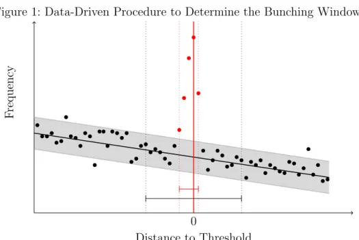
be asymmetric is that when individuals are risk-averse, we expect they are more likely to over-adjust their income to make sure they realise an income which is below the threshold. This psychological component will lead to an asymmetric bunching window, with more mass to the left of the threshold. A graphical intuition for our procedure is given in Figure 1. The binpoints around the threshold that have a higher actual number of taxpayers than predicted (coloured in red in Figure 1) are then used to determine the bunching window.
In order to determine the optimal bunching window, we propose the following step-wise procedure:
1. Set an excluded region around the threshold.
2. Run a local regression through all data bins outside the excluded region and predict
the values for z.
3. Compute a confidence interval around the prediction.
4. Subsequent bin midpoints outside the confidence interval comprise the bunching window.
4Using an optimal renders robustness checks with different bunching windows obsolete. To show the
Figure 1: Data-Driven Procedure to Determine the Bunching Window
Distance to Threshold
F
requency
0
Notes: This figure shows the bin midpoints as well as the fitted values of a linear regression. The grey confidence band is calculated with the standard errors of the point prediction. Here, five subsequent bin midpoints around the threshold lie outside and therefore determine the relevant (asymmetric) bunching window.
In general, the excluded region can be set arbitrarily, however we propose to iterate through different combinations of upper and lower bounds of the excluded region to
check for the sensitivity of the bunching window to the choice of the excluded region.5
The choice of the appropriate confidence interval is also at the researchers discretion, where higher confidence levels tend to lead to a smaller bunching window. In other words, the probability that we erroneously take individuals into the bunching window that do not bunch decreases. Depending on the setting and the data, this will lead to more conservative estimates of the elasticity.
We formally derive the bunching window as follows: Let x−∈ {−X,(−X+ 1), . . . ,0}
and x+ ∈ {0,1, . . . , X} be the lower and upper bound of the excluded region,
respect-ively. Furthermore, define l(x−, x+) as the lower bound of the bunching window and
u(x−, x+) as the upper bound of the bunching window, given the excluded region from
[x−, x+]. For every tuple (x−, x+), we run a local regression of polynomial orderq:
˜ NjBW = q X i=0 βiZji+εj ∀ j /∈[x−, x+]. (3)
We then predict the counterfactual values ˆNjBW and the standard error of the point prediction: ˆ NjBW = ˆβZj ∀j (4) ˆ SEf cst = v u u t( 1 n−1 n X j=1 ˆ ε2 j)(1 + 1 n). (5)
To allow for noise in the data, we calculate the upper value of the confidence interval
CIj+ for a given t-value using standard procedures. To determine the excess mass, we
subtract theCIj+ from the observed number of taxpayers in income bin j:
Ej =Nj−CIj+. (6)
If allEj are negative, no bunching is present in the sample. Otherwise, the lower bound
of the bunching window is given by:
l(x−, x+) = jl∗+ 1, where j
∗
l = max{j ∈Z−: Ej <0} (7)
which is the smallest subsequent income bin j that still satisfies the condition Ej > 0.
Similarly, the upper bound is given by:
u(x−, x+) = ju∗−1, where j
∗
u = min{j ∈Z+ : Ej <0} (8)
which is the largest subsequent income binj that still satisfies the condition Ej >0.
Through this procedure, we obtain several values for the lower and upper bounds of the bunching window that come from the different excluded regions. Several possibilities
arise as to which values of l(x−, x+) and u(x−, x+) to use as the limits of the bunching
window, but we advocate to use the mode of all estimated values. This ensures that in
most of the cases, we obtain the right bounds of the bunching window. 6 To estimate
the ETI from Equation (2), we need to obtain an estimate ofb, as the other parameters
from the equation are known policy parameters. We estimate b in the following way:
ˆ
b = PuBˆ lNˆj
(u−l+1)
, (9)
where our estimate of ˆB satisfies the integration constraint and ˆNj are the counterfactual
number of individuals within an income bin j that are determined by local polynomial
regression of the form:
6Other possibilities would be to use the minimum, maximum or mean, although we do not find large
ˆ Nj = q X i=0 βi·Zi+ u X i=l γi·I[Zj =i] +εj. (10)
2.3. Evaluation
We assess the validity of our endogenously determined bunching window by Monte Carlo simulations and evaluate the performance for two predictions: how well the approach can recover the true elasticities and how well it can identify the bunching individuals. Moreover, we test the robustness of our approach by varying the key parameters of the model. Especially, variations in the binwidth, the amount of frictions, the sample size and the size of the tax rate change at the threshold are examined.
The baseline specification has N = 1,000,000 observations, a threshold k at z =
50,000, a binwidth of 100, and the tax change is 10 percentage points7. We run
estima-tions for three different true elasticities, e= 0.02, e= 0.1 ande= 0.5. As the bunching
literature tends to find small elasticities, we only report the results fore = 0.02 here in
detail.
A comparison of the income distribution in case of a kink with a counterfactual scen-ario without a kink can be used to determine the elasticity (see Section 2.1). To abstract from any uncertainty regarding the counterfactual model, we randomly draw potential
incomesz0 from a triangular distribution.8 They are used to calculate the pre- and
post-reform taxable incomesz1 and z2 respectively, wherez1 =z2 for all individuals that are
at or below the kink, as they are not affected by the new tax system.9 We identify
all individuals as bunchers that have their highest post-reform utility at income level
k, provided they had z1 > k. To model optimisation frictions, we introduce a random
component in the income of the bunching individuals, described by ε ∼ N(0,142.3) in
our baseline specification.10
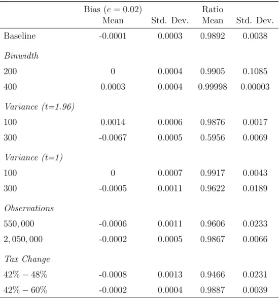
Table 1 shows the results of our Monte Carlo simulations. The columns present
the difference between the true and simulated elasticity as well as the ratio of identified bunchers over actual bunchers, which resembles an estimation error. Each row represents a different specification. In the baseline setting, the estimated elasticities have a mean
very close to the true elasticity of e = 0.02. At the same time, we are able to identify
7More specifically, the change is from 42% to 52%, resembling the change at the top tax threshold in
the Netherlands.
8Because we draw from a triangular distribution, we know that the counterfactual model is best
approximated by a linear model
9The choices of z
1 and z2 come from maximising a quasi-linear utility function. The approach is
similar to the approach taken in the working paper version of Bastani and Selin (2014).
10The variance component comes from the working paper version of Bastani and Selin (2014) and is
Table 1: Monte-Carlo Simulations of Elasticity
Bias (e = 0.02) Ratio
Mean Std. Dev. Mean Std. Dev.
Baseline -0.0001 0.0003 0.9892 0.0038 Binwidth 200 0 0.0004 0.9905 0.1085 400 0.0003 0.0004 0.99998 0.00003 Variance (t=1.96) 100 0.0014 0.0006 0.9876 0.0017 300 -0.0067 0.0005 0.5956 0.0069 Variance (t=1) 100 0 0.0007 0.9917 0.0043 300 -0.0005 0.0011 0.9622 0.0189 Observations 550,000 -0.0006 0.0011 0.9606 0.0233 2,050,000 -0.0002 0.0005 0.9867 0.0066 Tax Change 42%−48% -0.0008 0.0013 0.9466 0.0231 42%−60% -0.0002 0.0004 0.9887 0.0039
Notes: This table shows the results from the Monte Carlo simulations running 600 repetitions. Baseline consists of Binwidth 100, Variance 142.3, Observations 1,000,000 and Tax Change 42%-52%. All specifications use a t-value of 1.96, except the third, which uses t-value of 1. Note that a bias of zero indicates that the bias is less than 1/10000.
98.92% of the bunchers using our data-driven procedure. To assess the robustness of our approach we change the size of key parameters.
Throughout the bunching literature, several different binwidths are implemented. Many studies alter the binwidth in robustness checks and show limited sensitivity to changes in the binwidth (Chetty et al., 2011; Bastani and Selin, 2014). The results in Table 1 show that there are no significant changes regarding the estimated elasticities. A greater binwidth naturally improves the identification of the number of bunchers up to almost 100 %, but the number of individuals wrongly assumed as bunching also rises with an increased binwidth (bias-efficiency trade off).
Next to the binwidth, the variance that represents optimisation frictions could affect the performance of our data-driven procedure. Indeed, increasing the variance term in the randomised component, has a severe negative effect on the performance of the
bunching estimator. We estimate an elasticity of e = 0.013 which is far off the true
elasticity and are only able to identify 59.65% of the bunching taxpayers. A potential driver behind this could be the choice of the confidence interval. A high confidence interval should give us a narrow bunching window. But because the optimisation frictions are so high, we would expect a much wider range of the bunching window as well as a flatter area of excess mass around the kink point. Therefore in the third specification, we use a t-value of 1 instead of 1.96. The results improve significantly and our procedure is able to identify 96.22% of all bunching individuals when the variance term is 300. In light of this, the researcher should take the anticipated amount of optimisation frictions into account when setting the t-value for the confidence interval. For example, a more complex or dynamic tax system should lead to more optimisation frictions.
Due to its nonparametric nature, the bunching estimator relies on a large sample size. We test for the impact of different sample sizes on the efficiency of our estimation procedure. Unsurprisingly, an increased sample size increases efficiency, although the gains asymptotically decrease to zero.
The size of the tax change matters for overcoming optimisation frictions which cause the observed elasticity to differ from the structural elasticity (Chetty, 2012). As a bigger tax rate change has more severe consequences for the individuals we should observe more precise bunching with greater tax rate differences as the costs of adjusting taxable income are increasingly outweighed by the benefits (Chetty et al., 2011). With increasing size of the difference between the two marginal tax rates, we can identify the true elasticity more precise, confirming the results by Bastani and Selin (2014) and Chetty (2012) that larger jumps in the marginal tax rate are more informative of the true ETI.
3. Institutional Background
The Dutch tax system is almost fully individualised and tax liabilities mainly depend on individual worldwide income. There are a few exceptions, of which two are relevant for our analysis. First, means-tested subsidies such as health tax subsidy, child care subsidy and rental subsidy are all based on household taxable income. Second, personal tax-favoured expenditures can be shifted between partners, thereby reducing taxable income of the partner. This last possibility is attractive in a progressive tax schedule
such as the Dutch tax system for labour income.11
Since 2001, income from different sources is treated in three different “boxes” each with their own taxable income concept and tax schedule. In Box 1, income from profits, employment and home ownership is taxed. This includes wages, pensions and social transfers. Box 2 consists of income from substantial shareholding such as dividends and capital gains. Any other income from savings and investments is taxed in Box 3. Whilst income in Box 1 is taxed at progressive rates that jump up at certain thresholds and thus creating kinks in the tax schedule, income in Box 2 and Box 3 are subject to a flat
tax, which was 25% and 30% respectively in 2013.12 In our analysis, we use the kinks
in the Box 1 tax schedule for identification. It is furthermore worth noting that losses from different boxes cannot be offset against each other.
Income falling into Box 1 less personal deductions is taxed at progressive tax rates. The tax schedule in Box 1 consists of four tax brackets with increasing marginal tax rates. Figure 10 in the Appendix shows the development of the marginal tax rates over time. The two lower tax rates also include a general social security contribution of around 31% for old-age pensions and exceptional medical expenses. There is an increase in the marginal tax rate of 8%-points at the first threshold. Due to the social security contributions that apply in the second but not in the third tax bracket and a similar rise in the tax rate, marginal tax rates in the two brackets are similar. However, there is a large jump in marginal tax rates from 42% to 52% for the last bracket. In the considered time period, the income thresholds have been adjusted upwards to account for inflation and to avoid the cold progression phenomenon. For a better understanding of the tax schedule, Figure 2 provides an overview of the tax schedule that was in place in 2013. The marginal tax rate is given by the solid line and at each threshold, denoted by the dashed lines, the marginal tax rate jumps up, thus creating a kink in the budget set.
11From a labour supply perspective, a third exception is also relevant. A non-working spouse can
transfer the lump-sum tax credit to his or her partner. The moment the spouse starts working the first euro earned is taxed at the marginal tax rate. This is not the perspective taken in our study.
12We are aware of the possibility of shifting income between the boxes, which could be especially
pronounced for self-employed individuals. For the importance of shifting between tax bases see Harju and Matikka (2014). Due to data limitations, we cannot extend our analysis down that road.
Figure 2: Tax Schedule in 2013 Taxable Income MTR 19,645 33,363 55,991 10% 20% 30% 40% 50%
Notes: The figure shows the marginal tax rates for the year 2013. At each threshold, denoted by the dashed lines, the marginal tax rate jumps up.
One important channel of changing taxable income is legal tax avoidance by using deductions, such as pension contributions (Chetty et al., 2011). Other deduction pos-sibilities are alimonies paid, charitable givings, health expenditures or mortgage interest
deductions.13 In the Netherlands, the mortgage interest deduction is quite high and
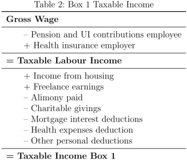
common among house-owners. More importantly, all of these deductions can be shifted between partners. An overview of the computation of taxable income is given in Table 2.
Important for any analysis looking at bunching is the exact tax payment procedure. It should be emphasised that for employees, the employer withholds income tax from Box 1 as a wage tax, which can be seen as a prepayment credited against the final tax amount at the end of the year. This third-party reporting is important for the interpretation of the results as systematic tax evasion, which is one possibility to adjust taxable income, becomes more difficult (Kleven et al., 2011). Final income taxes are determined after the end of the fiscal year, when tax deductions and income from other sources are taken
into account.14 An important distinction is single filing or joint filing. Even though
the Dutch tax system is rather individualised, married couples file jointly. In addition,
13These are (at least in parts) common in other countries like Great Britain or Germany as well. 14Note that the tax thresholds are known before the start of the fiscal year, as they are declared with
Table 2: Box 1 Taxable Income Gross Wage
– Pension and UI contributions employee + Health insurance employer
= Taxable Labour Income + Income from housing + Freelance earnings – Alimony paid – Charitable givings
– Mortgage interest deductions – Health expenses deduction – Other personal deductions = Taxable Income Box 1
Notes: This table shows the computation of Box 1 taxable income in the Netherlands.
also non-married cohabiting couples are allowed to make a joint tax filing. Taxes are filed digitally (computer-assisted) or on paper in the Netherlands, as is common in most developed countries. The share of digital filers has increased dramatically from about 30 percent in 2003 to almost 95 percent in 2015. Digital filing does not only help to deduct certain personal expenditures, but it also facilitates the optimal shifting. The exact location of the threshold becomes more salient and enables people to locate at the threshold.
To sum up, the Dutch tax system can evoke bunching behaviour due to the com-bination of three things. First, partners can shift deductions between them and this is most attractive in the highest income tax bracket. Second, there is a quite large mort-gage interest deduction. Third, it is very common to file digitally which makes the tax threshold as well as the related benefits of shifting more salient. As we will show, these specific features of the Dutch tax system result in sharp bunching at the third threshold.
4. Data
The data used in this paper is the Income Panel Data (IPO) provided by Statistics
Netherlands and covers the years 2001 to 2013. This longitudinal dataset contains
individual level administrative data on all sources of income that an individual might have, as well as a very detailed account of possible deductions from the tax base. The panel is updated with spouse and other randomly selected individuals in every period
to account for people who are no longer observable. Most importantly for this study, Statistics Netherlands provides the relevant taxable income for Box 1 (see Table 2). The taxable income variable comes from the tax authority and represents the exact amount of taxable income the individual is due. This circumvents the problem of measurement error, which is vital for analysis using the bunching method. As our income measure only includes relevant tax deductions, we do not have to rely on tax simulators used in other studies (Gruber and Saez, 2002; Chetty et al., 2011) to determine the tax liabilities, thus mitigating bias that could stem from this exercise.
In addition to the information on taxable income and deductions, the dataset also includes demographic characteristics, which we exploit to study heterogeneity in the bunching behaviour of different socio-economic groups. We use information on self-employed individuals, who are theoretically more prone to bunching due to the lower costs and greater possibilities of adjusting their taxable income. Furthermore, we dis-tinguish between genders and show results for married individuals. We restrict our estimation sample as follows. We exclude students as well as all people that receive any (governmental) transfers, as most of them receive transfers of similar height, thus creating an artificial mass point. Because the tax system changes for individuals aged 65 and over, we exclude them from our estimation as well as individuals below the age of 18. We exclude the years 2001 and 2002, because we suspect to pick up after effects
of the major tax reform in the Netherlands in 2001.15 Furthermore, we only keep
in-dividuals that have a positive reported taxable income. The pooled sample consists of
N = 1,219,572 individuals, which are roughly 1% of the Dutch population per year.
It is evenly balanced with respect to gender (55% are male) and married individuals constitute 65% of our sample. Furthermore, the sample consists of 14% self-employed individuals. This includes CEO’s that are also major shareholders of their firm, because they have the possibility to decide on their own salary and are flexible in adjusting it. Thus, they have the same possibility of adjusting their taxable income as self-employed individuals.
5. Results
5.1. Bunching Evidence
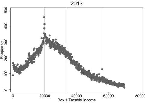
Figure 3 gives a first hint of bunching behaviour. It displays the income distribution for the most recent year of our sample. The threshold incomes of 2013 are indicated by vertical lines. We can see clear bunching behaviour at the first and third threshold.
15The tax reform changed the thresholds and marginal tax rates substantially and introduced the
Figure 3: Sample Income Distribution of 2013 0 100 200 300 400 500 Frequency 0 20000 40000 60000 80000
Box 1 Taxable Income
2013
Notes: This figure shows the sample distribution of income below 70,000 e in the Netherlands for 2013. The data is collapsed into 100 e bins. The vertical lines represent the first, second and third threshold of the Dutch tax system respectively.
Note that the change in the marginal tax rate at the second threshold is merely 1.08% and so the incentive for adjusting taxable income is small. For this figure and the rest
of the analysis the data is collapsed into income bins of 100e.16
Upper Threshold
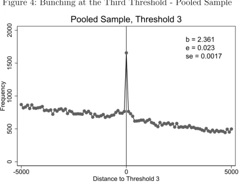
The change in the tax rate is largest at the upper threshold of the Dutch tax schedule with 10%-points (23.81%), which implies that bunching behaviour should be more pro-nounced here. We report the results for our pooled sample from 2003 to 2013 in Figure 4. The figure shows the number of observations per bin, relative to the threshold value. For pooled years, our method to endogenously determine the bunching window provides
an asymmetric bunching window ranging from -550e to +350e. We implement a 95%
confidence interval for determining the bunching window throughout this paper.17 The
BIC criterion suggests a linear counterfactual model, which can be explained by the location of the kink point at right tail of the income distribution. In order to calculate
16Our results are not driven by the selection of this binwidth. For higher binwidths (200 and 400), the
bunching window would be smaller and similar estimates of the elasticity are obtained, although the value ofbvaries with the binwidth.
17We also tested a smaller confidence level, i.e. a one-standard deviation increase, which corresponds
an elasticity, a weighted average threshold value is used. The weights are the number of taxpayers exactly at the threshold in each year, i.e. in income bin 0. Standard errors are calculated with a parametric residual bootstrap procedure.
Figure 4: Bunching at the Third Threshold - Pooled Sample
0 500 1000 1500 2000 Frequency -5000 0 5000 Distance to Threshold 3
Pooled Sample, Threshold 3
b = 2.361 e = 0.023 se = 0.0017
Notes: This figure plots bin counts relative to the threshold for the pooled sample from 2003 to 2013. The data is collapsed into 100 ebins. The bunching window is between -550eand +350eand the counterfactual model is linear.
We observe sharp bunching at the threshold and estimate an excess mass of taxpayers
at the threshold of b = 2.36, which corresponds to 2.36 times more individuals being
at the threshold than would have been in the absence of the tax change. This excess mass implies an ETI with respect to the net-of-tax rate of 0.023, which is statistically significant at all usual significance levels. Quantitatively, a decrease in the net-of-tax rate by 10% induces a reduction of taxable income by 0.23%.
Other Thresholds
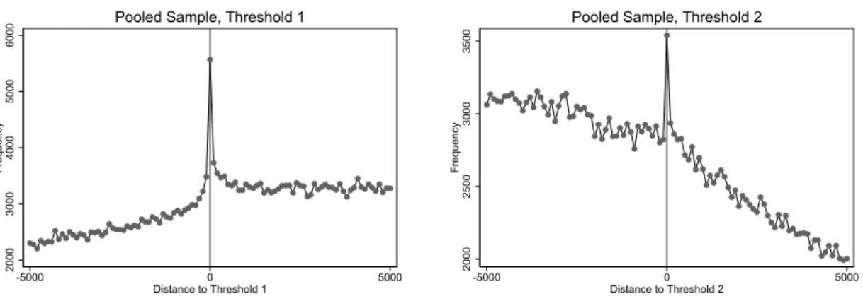
A case could be made for bunching at the other thresholds of the Dutch tax system as well. Our a priori hypothesis is that we should observe limited bunching at the other two thresholds. At the second threshold, the change in the tax rate is very small, especially in the more recent years, as shown in Figure 10 of the Appendix. At the first threshold, the income levels are quite low, which would suggest that most individuals need their
full income for a living and should react insensitive to changes in the marginal tax rate.18
Figure 5: Bunching at the First and Second Threshold - Pooled Sample 2000 3000 4000 5000 6000 Frequency -5000 0 5000 Distance to Threshold 1
Pooled Sample, Threshold 1
2000 2500 3000 3500 Frequency -5000 0 5000 Distance to Threshold 2
Pooled Sample, Threshold 2
Notes: The figures show bunching at the first and second threshold for the pooled sample from 2003 to 2013. Due to the varying tax changes at these thresholds, no excess mass is reported.
Figure 5 shows the graphs for the pooled sample. Surprisingly, we observe bunching behaviour of individuals at both thresholds. We cannot display exact estimates for the excess mass or the elasticities at these thresholds, because we have changing tax differences over time on top of the changing threshold values. Taking the average of the single-year estimations delivers an excess mass of 1.55 at the first threshold and
0.47 at the second threshold.19 Especially at the first threshold, the estimated average
excess mass is comparable to the single-year average excess mass at the third threshold, which translates into a significantly higher elasticity given the smaller tax change at the first threshold. A possible explanation for this is that many second or part-time earners could realise an income around this level. Given that they are not dependent on this income, these individuals are less constraint than we assumed. To confirm this, we estimate the ETI at the first threshold for married individuals. The elasticity is
estimated at e = 0.075 using a 7th order polynomial counterfactual and a bunching
window from −250e to +750e, as well as average marginal tax rates. The elasticity
at the first threshold is more than three times the elasticity of married individuals at
the third threshold (e = 0.021). This is clear evidence in favour of the second earner
hypothesis. The effect is especially pronounced for married women, which is shown in Figure 6.
The graph sheds further light on two things. First of all, there are less single than married individuals at the first threshold, but this could also be due to the higher number of married individuals in our sample. The distribution between women and
more pre-tax income will lead to more disposable income.
19The tax rate change at the second threshold is very small, therefore, as shown in the Monte Carlo
Figure 6: Bunching by Gender and Marital Status 0 2000 0 2000 -2000 -1000 0 1000 2000 -2000 -1000 0 1000 2000
Women, non-married Women, married
Men, non-married Men, married
Frequency
Distance to Threshold 1
Notes: The figures show bunching at the first threshold by gender and marital status.
men (top- and bottom-left figures) is relatively equal for non-married (meaning singles and unmarried, cohabiting couples) taxpayers. For the married individuals however, a significantly greater share of women bunches at the first threshold. This indicates that often women are the second earners and relates to earlier findings by Chetty et al. (2011), who also find significantly higher bunching of married women.
5.2. Sensitivity Analysis
One concern that could arise is that when pooling the data, we observe many individuals more than once. If for example a contract is signed for several years, which specifies that the salary moves along with the threshold, we would attribute bunching behaviour in every period to this individual, although the behavioural decision was made only once. This could possibly lead to an overestimation of the excess mass. To hedge against this, we randomly kept one observation per individual and reestimated the excess mass in the pooled sample. The excess mass drops to 2.02, which is in mild support of this hypothesis, but this could also be driven by the smaller sample size.
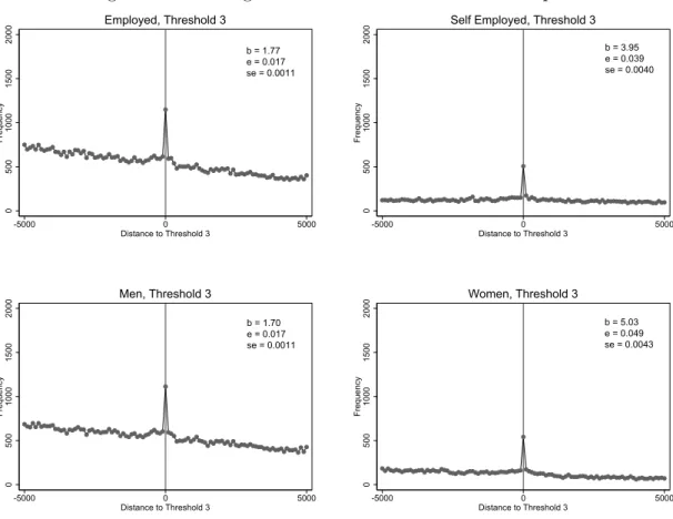
To analyse if our results are driven by subgroups, we split the sample by employment status and sex. On the one hand, self-employed individuals have better possibilities to adjust their taxable income and are therefore more prone to bunching. On the other hand, women, who are often second earners, are also more sensitive to changes in tax-ation. The results are shown in Figure 7. Our results confirm the hypotheses, as the excess mass for the self-employed increases significantly to 3.95 compared to the baseline analysis of the pooled sample. Contrary to many other studies, we also find a significant excess mass for wage employed individuals of 1.77, so the baseline result is not purely driven by self-employed individuals. The observed bunching for wage employees can be seen as an indication that collusion between the employer and the employee is present and contracts are specifically designed to achieve a taxable income at the threshold. Another explanation could be the existence of unions that jointly set wages for a group of individuals. The argument here is that collective knowledge in the union would make the individual optimisation errors less pronounced and therefore lead to more (precise) bunching. An alternative explanation is that wage employees also utilise tax deductions. The bottom two graphs in Figure 7 are clear evidence in favour of the gender difference hypothesis, as the excess mass of women at the third threshold is 5.03, whilst the excess mass for men is only 1.70. For self-employed women, the excess mass rises to 7.17 (not depicted) and is still significant, but due to the very small sample size, this result should be viewed with caution.
We estimate the excess mass of taxpayers and the ETI at the third threshold for all years separately. This hedges against the concern that we use a weighted average threshold in the pooled sample to obtain our elasticity estimate. The results are relegated to the Appendix (Figure 9 and Table 3). One striking observation is that the bunching behaviour of individuals increases and becomes more precise over time. We ascribe this to learning effects as the taxpayers become more familiar with the tax system. In the year 2002 we still observe delayed effects from the major tax reform of 2001 and therefore, the bunching behaviour is fuzzy and small. It then increases in the subsequent years until the excess mass reaches a level of around 2, corresponding to an elasticity of 0.02. Another explanation could be the emergence of digital filing, which made the threshold more salient to the general public.
5.3. Anatomy of Response
The channels through which individuals bunch at thresholds of a tax system are mani-fold. In order to reduce taxable income, individuals could work less hours, which, from an efficiency point of view, would be an undesirable effect of the threshold. On the other hand, tax liabilities can be reduced by shifting income either over time or across
Figure 7: Bunching at the Third Threshold - Subsamples 0 500 1000 1500 2000 Frequency -5000 0 5000 Distance to Threshold 3 Employed, Threshold 3 b = 1.77 e = 0.017 se = 0.0011 0 500 1000 1500 2000 Frequency -5000 0 5000 Distance to Threshold 3
Self Employed, Threshold 3 b = 3.95 e = 0.039 se = 0.0040 0 500 1000 1500 2000 Frequency -5000 0 5000 Distance to Threshold 3 Men, Threshold 3 b = 1.70 e = 0.017 se = 0.0011 0 500 1000 1500 2000 Frequency -5000 0 5000 Distance to Threshold 3 Women, Threshold 3 b = 5.03 e = 0.049 se = 0.0043
Notes: The figures show bunching at the third threshold from 2003 to 2013 for different subsamples. The bunching window for the employed sample is between -550eand +250eand the counterfactual model is linear. The bunching window for the self-employed sample is between -550 e and +150 e and the counterfactual is a second order polynomial model. The bunching window for the male sample is between -550 eand +250e and the counterfactual model is linear. The bunching window for the female sample is between -550eand +350eand the counterfactual model is linear.
individuals (if joint taxation components exist) or by (itemized) tax deductions. A recent study by Doerrenberg et al. (2015) show the importance of tax deductions for welfare analyses with the ETI. As pointed out by Slemrod (1996), one way to illicit the channel that drives bunching is to look at the “anatomy of the behavioural response” (Saez et al., 2012). We analyse the anatomy of response of wage earners for the period 2004 to 2011. Of all wage-earners in the vicinity of the third threshold, almost 71% pay deductible mortgage interest. Some smaller part also earns self-employment income and a few deduct other expenditures such as health expenditures or charitable givings. For about 14 percent, we cannot identify their source of bunching. This could be attributed
to the way deductions are observed in the data20 or that the source of bunching could
be driven by a real response such as a reduction in working hours instead of income shifting.
It is worthwhile to examine the mortgage interest deduction, which can only be claimed for the first mortgage taken out, more closely. Because of the progressive tax system, shifting income to the partner can be financially attractive. In general, shifting the full deduction to the highest earning partner will reduce tax liabilities most. However, the actual incentive depends on the distance of taxable income to the threshold. Suppose the highest earning partner starts using the tax deduction to reduce his taxable income. Once he reaches the threshold he can do two things. Either he can deduct the rest at a lower marginal tax rate or he can shift the rest to his partner. If his partner earns less than the second threshold, he fully deducts the interest payment. If his partner earns more than the second but less than the third threshold then shifting does not matter. If however, his partner earns more than the third threshold the tax deduction should be
shifted. This last case will result in sharp bunching at the third threshold.21
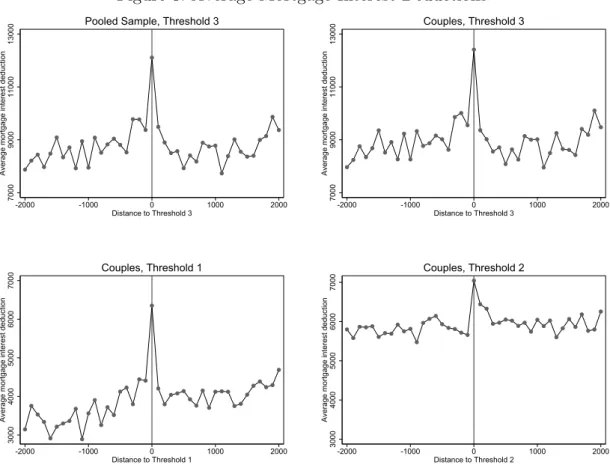
The sharp bunching is clearly visible in Figure 8. These top graphs show the average mortgage interest deduction for each bin around the upper tax threshold for the pooled sample and the sub-sample of couples respectively. The average mortgage interest de-duction is highest at the threshold. The figures show that the effect in the pooled sample is driven by individuals living in couples. At the other thresholds (shown in the bottom graphs) we also observe an increase in the mortgage interest deduction, especially at the first threshold. Surprisingly there appears to be a higher mortgage interest deduc-tion even at threshold 2, where the tax incentive is small. One of the reasons is that in the early years of our sample, the tax increase was bigger. In line with intuition,
20We underestimate the share because for some couples we do not observe the actual mortgage interest
deduction. In case both partners deduct mortgage interest, Statistics Netherlands assigns the sum of these deductions to the partner that earns a higher income. This is done regardless of the distance to the threshold and as such poses no problem for our analysis.
21This line of argumentation also holds for partners having similar incomes just above the other
Figure 8: Average Mortgage Interest Deductions
7000
9000
11000
13000
Average mortgage interest deduction
-2000 -1000 0 1000 2000 Distance to Threshold 3
Pooled Sample, Threshold 3
7000
9000
11000
13000
Average mortgage interest deduction
-2000 -1000 0 1000 2000 Distance to Threshold 3 Couples, Threshold 3 3000 4000 5000 6000 7000
Average mortgage interest deduction
-2000 -1000 0 1000 2000 Distance to Threshold 1 Couples, Threshold 1 3000 4000 5000 6000 7000
Average mortgage interest deduction
-2000 -1000 0 1000 2000 Distance to Threshold 2
Couples, Threshold 2
Notes: The top figures show average mortgage interest deductions for all workers (left) and workers living in couples (right) around the third threshold. The bottom figures show average mortgage interest deductions for workers living in couples for the first (left) and second (right) threshold.
the mortgage interest deductions are highest for the top threshold, where the marginal tax rate changes most significantly. Although lower in absolute terms, the jump at the
first threshold is similar to the jump at the third threshold (around 2,000eon average,
compared to the neighbouring data points). The mortgage interest deductions thus are an important channel for reducing taxable income to reach thresholds of a tax system.
A second possible channel are responses in hours worked. Due to the structure of our data, identification of responses in hours can only be done indirectly, for example via hourly wages. As bunchers come from above the threshold and we can assume that hourly wage increases with taxable income, i.e. a higher taxable income is associated with a higher hourly wage, an individual that bunches should have a higher hourly wage than other individuals working the same hours. Looking at data from 2006 to 2011, we cannot identify a significant difference between bunching employees and non-bunchers in terms of hourly wages.
5.4. Relation to the Literature
Our results relate to the literature in several ways, although cross country comparisons of elasticities might be difficult due to different institutional features (Bastani and Selin, 2014). In line with other studies that implement the bunching approach, we find small but precise estimates of the compensated ETI with respect to the net-of-tax rate at the
top tax threshold of 0.023. Chetty et al. (2011) find an elasticity at the upper threshold
below 0.02 for their full sample in Denmark, whilst Bastani and Selin (2014) find close to
zero-elasticities in Sweden at the top tax threshold. Evidence for the US by Saez (2010)
indicates an elasticity between 0.1 and 0.2, depending on the methodology, at the first
threshold of the federal income tax schedule. It is slightly lower for married individuals and is thus in stark contrast to our results that indicate significant bunching by married individuals even at the first threshold of the tax system in the Netherlands.
One structural difference that can explain this deviation between the US and the Netherlands is the social acceptance and federal legitimation of part-time work. Whilst in the US only 19% of the working population was working part-time in 2013, in the Netherlands this figure was almost twice as high with 36%. The significantly larger proportion of (married) women bunching can also be explained by this. In the US, 26% of the female workforce worked part-time but in the Netherlands, 58% worked part-time
and would more likely earn an income close to the first threshold.22 This could be a
reason for the differences in the results. Alternative explanations are differences in other institutional features such as the possibility to shift deductions to the partner or the
22The shares are calculated from the OECD Statistics database, where the labour force is measured by
presence of digital filing.
Earlies studies for the Netherlands find larger elasticities. Jongen and Stoel (2013) find an elasticity of around 0.1 in the short run and 0.2 in the medium run. This study employs a panel approach and uses instrumental variable techniques to correct for endogenous taxes in the spirit of Gruber and Saez (2002). Consistent with our estimates, they also find higher elasticities for women. Contrary to our study, the authors had to rely on a tax simulator to obtain marginal tax rates and determine taxable income. This can potentially cause measurement error, which could explain some of the deviation between the results. Another explanation would be that the bunching approach identifies a local elasticity as opposed to a more structural elasticity derived from the IV approach. A recent study by Bettendorf et al. (2015) for managing directors that own at least 5%
of a corporation23 finds elasticities between 0.06 and 0.11 for the upper threshold of the
Dutch tax schedule using bunching techniques. This is slightly larger than the elasticity of 0.04 that we identify for self-employed individuals and could suggest that our results are partly driven by the DGA subgroup. Unfortunately, the limited number of DGA’s in our sample prevents us from running the estimation separately for this group.
In all bunching analyses the distinction is made between real response and income shifting. Le Maire and Schjerning show in a study on Danish self-employed that about 50-70% of the bunching in taxable income is due to income shifting (Le Maire and Schjerning, 2013). We however find that a large- but not full - share of bunching is driven by tax deductions. The presence of deduction possibilities confounds welfare analyses using the ETI (Doerrenberg et al., 2015). Our results confirm the significance of deduction possibilities for optimising taxable income. This finding mirrors earlier findings on itemized deductions (Saez, 2010).
We further interpret our results as little support for collusion between employers and employees. As final income taxes are based on taxable income and not on broad income on the wage bill, it is harder to pinpoint the exact taxable income by employers and employees. The same holds for hourly responses. Although employees can more easily adjust hours in the Netherlands than in other countries, adjusting hours in such a way as to locate at the threshold is very hard. It requires an extensive knowledge of the tax thresholds and the amount of all the deductions that turn taxable labour income into taxable income Box 1. Nevertheless, hourly responses could play a role when analysing self-employed, but due to a lack of data on hours worked by self-employed, we are not able to test this hypothesis. Our results indicate that shifting of deductions and more specifically shifting of deductions between partners is the key to understanding bunching behaviour in the Netherlands.
23These so-called DGA (Directeur-Grootaandeelhouder) face a special tax scheme. In our study, this
6. Concluding Remarks
In this paper we have estimated the (compensated) elasticity of taxable income with respect to the net-of-tax rate in the Netherlands. Using a unique data set from Statistics Netherlands containing exact taxable income, we exploited bunching behaviour at kink points of the Dutch tax schedule. We found an excess mass of 2.36 and a corresponding elasticity of 0.023. With an excess mass of 3.95 for the self-employed and 5.03 for women, the estimates are in line with the third-party reporting hypothesis and further suggest that women are more responsive to taxation. Our findings are quantitatively similar to recent studies exploiting bunching with one exception. While Chetty et al. (2011) for Denmark or Bastani and Selin (2014) for Sweden find a nearly zero elasticity for wage earners, we find a small, yet statistically significant estimate of 0.02 for wage earners in the Netherlands. Further exploration of the anatomy of response for wage employees revealed that bunching is caused by shifting deductions between partners. Shifting is facilitated by digital filing which makes the thresholds more salient. This results corroborates earlier studies who claim that the ETI is not a structural parameter but depends on institutional settings.
We have also contributed methodologically in two ways. Elasticities derived with the bunching approach heavily rely on both the estimated counterfactual density and the determination of the bunching window. To improve the reliability of the bunching es-timation, we first proposed to choose the counterfactual model based on the information criteria. Second, we implemented an intuitive, purely data-driven procedure to find an optimal bunching window. Applying these extensions to our data, we found elasticities that are marginally smaller, yet statistically more significant. Our modifications are thus a valuable contribution to the literature as they allow for a more precise calculation of the excess mass at the kink.
Overall, our empirical results showed that the Dutch population responds to taxation and adjusts their taxable income. For employees, we could identify the mortgage interest deduction as the main channel through which taxable income is adjusted. An adjustment of hours worked could not be inferred from the data, but such real responses and even evasion remain potential channels for self-employed, where the income is not reported by a third-party.
References
Adam, S., J. Browne, D. Phillips, and B. Roantree(2015): “Adjustment costs
and labour supply: evidence from bunching at tax thresholds in the UK,” mimeo.
Bastani, S. and H. Selin(2014): “Bunching and non-bunching at kink points of the
Swedish tax schedule,” Journal of Public Economics, 109, 36–49.
Bettendorf, L. J. H., A. Lejour, and M. van’t Riet(2015): “Tax bunching by
owners of small corporations,” mimeo.
Chetty, R.(2012): “Bounds on Elasticities With Optimization Frictions: A Synthesis
of Micro and Macro Evidence on Labor Supply,” Econometrica, 80, 969–1018.
Chetty, R., J. N. Friedman, T. Olsen, and L. Pistaferri(2011): “Adjustment
Costs, Firm Responses, and Micro vs. Macro Labor Supply Elasticities: Evidence
from Danish Tax Records.” The Quarterly Journal of Economics, 126, 749–804.
Doerrenberg, P., A. Peichl, and S. Siegloch (2015): “The elasticity of taxable
income in the presence of deduction possibilities,” Journal of Public Economics.
Feldstein, M.(1995): “The Effect of Marginal Tax Rates on Taxable Income: A Panel
Study of the 1986 Tax Reform Act,” Journal of Political Economy, 103, 551–72.
Gruber, J. and E. Saez (2002): “The elasticity of taxable income: Evidence and
implications,” Journal of Public Economics, 84, 1–32.
Harju, J. and T. Matikka (2014): “The Elasticity of Taxable Income and
Income-shifting: What is” real” and what is Not?” in Personal Income Taxation and
House-hold Behavior (TAPES), American Economic Journal: Economic Policy (American Economic Association).
Jongen, E. L. W. and M. Stoel (2013): “Estimating the Elasticity of Taxable
Labour Income in the Netherlands,” CPB Background Document.
Kleven, H. J., M. B. Knudsen, C. T. Kreiner, S. Pedersen, and E. Saez (2011): “Unwilling or unable to cheat? Evidence from a tax audit experiment in
Denmark,” Econometrica, 79, 651–692.
Le Maire, D. and B. Schjerning (2013): “Tax bunching, income shifting and
self-employment,” Journal of Public Economics, 107, 1–18.
Saez, E.(2010): “Do Taxpayers Bunch at Kink Points?” American Economic Journal:
Saez, E., J. Slemrod, and S. H. Giertz (2012): “The Elasticity of Taxable
In-come with Respect to Marginal Tax Rates: A Critical Review,” Journal of Economic
Literature, 50, pp. 3–50.
Slemrod, J.(1996): “High-income families and the tax changes of the 1980s: the
ana-tomy of behavioral response,” in Empirical foundations of household taxation,
Uni-versity of Chicago Press, 169–192.
——— (1998): “Methodological issues in measuring and interpreting taxable income
elasticities,” National Tax Journal, 773–788.
Weber, C. E. (2014): “Does the Earned Income Tax Credit Reduce Saving by
A. Appendix
A.1. Additional Graphs and Tables
Figure 9: Bunching at the Third Threshold - Single Years
0 50 100 150 200 Frequency 42000 44000 46000 48000 50000 52000 Box 1 Taxable Income
2002, Threshold 3 0 50 100 150 200 Frequency 44000 46000 48000 50000 52000 54000 Box 1 Taxable Income
2003, Threshold 3 0 50 100 150 200 Frequency 46000 48000 50000 52000 54000 56000 Box 1 Taxable Income
2004, Threshold 3 b= 0.42,e= 0.0047,se= 0.0002 b= 0.41,e= 0.0044,se= 0.0002 b= 0.92,e= 0.0096,se= 0.0003 0 50 100 150 200 Frequency 46000 48000 50000 52000 54000 56000 Box 1 Taxable Income
2005, Threshold 3 0 50 100 150 200 Frequency 48000 50000 52000 54000 56000 58000 Box 1 Taxable Income
2006, Threshold 3 0 50 100 150 200 Frequency 48000 50000 52000 54000 56000 58000 Box 1 Taxable Income
2007, Threshold 3 b= 1.98,e= 0.0202,se= 0.0008 b= 1.80,e= 0.0183,se= 0.0007 b= 1.77,e= 0.0176,se= 0.0007 0 50 100 150 200 Frequency 50000 55000 60000
Box 1 Taxable Income
2008, Threshold 3 0 50 100 150 200 Frequency 50000 52000 54000 56000 58000 60000 Box 1 Taxable Income
2009, Threshold 3 0 50 100 150 200 Frequency 50000 52000 54000 56000 58000 60000 Box 1 Taxable Income
2010, Threshold 3 b= 1.35,e= 0.013,se= 0.0004 b= 2.42,e= 0.0234,se= 0.0009 b= 1.52,e= 0.0148,se= 0.0005 0 50 100 150 200 Frequency 50000 52000 54000 56000 58000 60000 Box 1 Taxable Income
2011, Threshold 3 0 50 100 150 200 Frequency 52000 54000 56000 58000 60000 62000 Box 1 Taxable Income
2012, Threshold 3 0 50 100 150 200 Frequency 50000 55000 60000
Box 1 Taxable Income
2013, Threshold 3
Table 3: Bunching Window and Counterfactual for Figure 9
Year Bunching Window Counterfactual Model
2002 -50 e to +50 e linear 2003 -50 e to +50 e linear 2004 -50 e to +50 e linear 2005 -50 e to +50 e Third-Order Polynomial 2006 -150 e to +50e linear 2007 -150 e to +50e linear 2008 -50 e to +50 e linear 2009 -150 e to +50e linear 2010 -50 e to +50 e linear 2011 -150 e to +250 e Second-Order Polynomial 2012 -50 e to +250 e linear 2013 -50 e to +150 e Second-Order Polynomial
Figure 10: Development of Marginal Tax Rates
Table 4: Comparison of Different Model Specifications (1) (2) (3) Sample b e se t b e se t b e se t Pooled Sample 2.36 0.0231 0.0017 13.83 2.23 0.0218 0.0087 2.08 1.96 0.0192 0.0035 5.08 Employed 1.77 0.0174 0.0011 15.65 1.85 0.0181 0.0070 2.16 1.61 0.0157 0.0027 5.34 Self-Employed 3.95 0.0387 0.0040 9.68 3.75 0.0367 0.0169 1.83 3.38 0.0331 0.0072 4.18 Men 1.70 0.0166 0.0011 15.59 1.55 0.0152 0.0064 1.99 1.46 0.0143 0.0025 5.30 Women 5.03 0.0492 0.0043 11.54 5.11 0.0499 0.0203 2.04 4.01 0.0392 0.0084 4.21
Notes: (1) represents our model with the endogenous bunching window and the counterfactual model, which is determined by the BIC. (2) show the results for a symmetric bunching window going from -750eto +750eand using a 7th order polynomial counterfactual model. (3) show the results for a symmetric bunching window going from -350eto +350eand using a 7th order polynomial counterfactual model. b is the estimated excess mass,ethe corresponding elasticity, sethe standard error obtained from a parametric residual bootstrap procedure andtis a t-value, obtained by dividing the elasticity by the standard error.
Hohenheim Discussion Papers in Business, Economics and Social Sciences
The Faculty of Business, Economics and Social Sciences continues since 2015 the established “FZID Discussion Paper Series” of the “Centre for Research on Innovation and Services (FZID)” under the name “Hohenheim Discussion Papers in Business, Economics and Social Sciences”.
Institutes
510 Institute of Financial Management 520 Institute of Economics
530 Institute of Health Care & Public Management 540 Institute of Communication Science
550 Institute of Law and Social Sciences
560 Institute of Economic and Business Education 570 Institute of Marketing & Management
580 Institute of Interorganisational Management & Performance
Download Hohenheim Discussion Papers in Business, Economics and Social Sciences from our homepage: https://wiso.uni-hohenheim.de/papers
Nr. Autor Titel Inst.
01-2015 Thomas Beissinger, Philipp Baudy
THE IMPACT OF TEMPORARY AGENCY WORK ON TRADE UNION WAGE SETTING:
A Theoretical Analysis
520
02-2015 Fabian Wahl PARTICIPATIVE POLITICAL INSTITUTIONS AND
CITY DEVELOPMENT 800-1800
520
03-2015 Tommaso Proietti, Martyna Marczak, Gianluigi Mazzi
EUROMIND-D: A DENSITY ESTIMATE OF
MONTHLY GROSS DOMESTIC PRODUCT FOR THE EURO AREA
520
04-2015 Thomas Beissinger, Nathalie Chusseau, Joël Hellier
OFFSHORING AND LABOUR MARKET REFORMS: MODELLING THE GERMAN EXPERIENCE
520
05-2015 Matthias Mueller, Kristina Bogner, Tobias Buchmann, Muhamed Kudic
SIMULATING KNOWLEDGE DIFFUSION IN FOUR STRUCTURALLY DISTINCT NETWORKS
– AN AGENT-BASED SIMULATION MODEL
520
06-2015 Martyna Marczak, Thomas Beissinger
BIDIRECTIONAL RELATIONSHIP BETWEEN INVESTOR SENTIMENT AND EXCESS RETURNS: NEW EVIDENCE FROM THE WAVELET PERSPECTIVE
520
07-2015 Peng Nie,
Galit Nimrod, Alfonso Sousa-Poza
INTERNET USE AND SUBJECTIVE WELL-BEING IN CHINA
530
08-2015 Fabian Wahl THE LONG SHADOW OF HISTORY
ROMAN LEGACY AND ECONOMIC DEVELOPMENT – EVIDENCE FROM THE GERMAN LIMES
Nr. Autor Titel Inst.
10-2015 Kristina Bogner THE EFFECT OF PROJECT FUNDING ON
INNOVATIVE PERFORMANCE
AN AGENT-BASED SIMULATION MODEL
520
11-2015 Bogang Jun,
Tai-Yoo Kim
A NEO-SCHUMPETERIAN PERSPECTIVE ON THE
ANALYTICAL MACROECONOMIC FRAMEWORK:
THE EXPANDED REPRODUCTION SYSTEM
520
12-2015 Volker Grossmann
Aderonke Osikominu Marius Osterfeld
ARE SOCIOCULTURAL FACTORS IMPORTANT FOR STUDYING A SCIENCE UNIVERSITY MAJOR?
520
13-2015 Martyna Marczak
Tommaso Proietti Stefano Grassi
A DATA–CLEANING AUGMENTED KALMAN FILTER FOR ROBUST ESTIMATION OF STATE SPACE MODELS
520
14-2015 Carolina Castagnetti Luisa Rosti
Marina Töpfer
THE REVERSAL OF THE GENDER PAY GAP AMONG PUBLIC-CONTEST SELECTED YOUNG EMPLOYEES
520
15-2015 Alexander Opitz DEMOCRATIC PROSPECTS IN IMPERIAL RUSSIA:
THE REVOLUTION OF 1905 AND THE POLITICAL STOCK MARKET
520
01-2016 Michael Ahlheim, Jan Neidhardt
NON-TRADING BEHAVIOUR IN CHOICE EXPERIMENTS
520
02-2016 Bogang Jun,
Alexander Gerybadze, Tai-Yoo Kim
THE LEGACY OF FRIEDRICH LIST: THE EXPANSIVE REPRODUCTION SYSTEM AND THE KOREAN HISTORY OF INDUSTRIALIZATION
520
03-2016 Peng Nie,
Alfonso Sousa-Poza
FOOD INSECURITY AMONG OLDER EUROPEANS: EVIDENCE FROM THE SURVEY OF HEALTH, AGEING, AND RETIREMENT IN EUROPE
530
04-2016 Peter Spahn POPULATION GROWTH, SAVING, INTEREST RATES
AND STAGNATION. DISCUSSING THE EGGERTSSON-MEHROTRA-MODEL
520
05-2016 Vincent Dekker, Kristina Strohmaier, Nicole Bosch
A DATA-DRIVEN PROCEDURE TO DETERMINE THE BUNCHING WINDOW – AN APPLICATION TO THE NETHERLANDS
FZID Discussion Papers
(published 2009-2014)
Competence Centers
IK Innovation and Knowledge
ICT Information Systems and Communication Systems
CRFM Corporate Finance and Risk Management
HCM Health Care Management
CM Communication Management
MM Marketing Management
ECO Economics
Download FZID Discussion Papers from our homepage: https://wiso.uni-hohenheim.de/archiv_fzid_papers
Nr. Autor Titel CC
01-2009 Julian P. Christ NEW ECONOMIC GEOGRAPHY RELOADED:
Localized Knowledge Spillovers and the Geography of Innovation
IK
02-2009 André P. Slowak MARKET FIELD STRUCTURE & DYNAMICS IN INDUSTRIAL
AUTOMATION
IK
03-2009 Pier Paolo Saviotti, Andreas Pyka
GENERALIZED BARRIERS TO ENTRY AND ECONOMIC DEVELOPMENT
IK
04-2009 Uwe Focht, Andreas Richter and Jörg Schiller
INTERMEDIATION AND MATCHING IN INSURANCE MARKETS HCM
05-2009 Julian P. Christ, André P. Slowak
WHY BLU-RAY VS. HD-DVD IS NOT VHS VS. BETAMAX: THE CO-EVOLUTION OF STANDARD-SETTING CONSORTIA
IK
06-2009 Gabriel Felbermayr, Mario Larch and Wolfgang Lechthaler
UNEMPLOYMENT IN AN INTERDEPENDENT WORLD ECO
07-2009 Steffen Otterbach MISMATCHES BETWEEN ACTUAL AND PREFERRED WORK
TIME: Empirical Evidence of Hours Constraints in 21 Countries
HCM
08-2009 Sven Wydra PRODUCTION AND EMPLOYMENT IMPACTS OF NEW
TECHNOLOGIES – ANALYSIS FOR BIOTECHNOLOGY
IK
09-2009 Ralf Richter, Jochen Streb
CATCHING-UP AND FALLING BEHIND KNOWLEDGE SPILLOVER FROM AMERICAN TO GERMAN MACHINE TOOL MAKERS
Nr. Autor Titel CC
10-2010 Rahel Aichele, Gabriel Felbermayr
KYOTO AND THE CARBON CONTENT OF TRADE ECO
11-2010 David E. Bloom, Alfonso Sousa-Poza
ECONOMIC CONSEQUENCES OF LOW FERTILITY IN EUROPE HCM
12-2010 Michael Ahlheim, Oliver Frör
DRINKING AND PROTECTING – A MARKET APPROACH TO THE
PRESERVATION OF CORK OAK LANDSCAPES ECO
13-2010 Michael Ahlheim, Oliver Frör, Antonia Heinke, Nguyen Minh Duc, and Pham Van Dinh
LABOUR AS A UTILITY MEASURE IN CONTINGENT VALUATION STUDIES – HOW GOOD IS IT REALLY?
ECO
14-2010 Julian P. Christ THE GEOGRAPHY AND CO-LOCATION OF EUROPEAN
TECHNOLOGY-SPECIFIC CO-INVENTORSHIP NETWORKS
IK
15-2010 Harald Degner WINDOWS OF TECHNOLOGICAL OPPORTUNITY
DO TECHNOLOGICAL BOOMS INFLUENCE THE RELATIONSHIP BETWEEN FIRM SIZE AND INNOVATIVENESS?
IK
16-2010 Tobias A. Jopp THE WELFARE STATE EVOLVES:
GERMAN KNAPPSCHAFTEN, 1854-1923
HCM
17-2010 Stefan Kirn (Ed.) PROCESS OF CHANGE IN ORGANISATIONS THROUGH
eHEALTH
ICT
18-2010 Jörg Schiller ÖKONOMISCHE ASPEKTE DER ENTLOHNUNG
UND REGULIERUNG UNABHÄNGIGER VERSICHERUNGSVERMITTLER
HCM
19-2010 Frauke Lammers,
Jörg Schiller
CONTRACT DESIGN AND INSURANCE FRAUD: AN EXPERIMENTAL INVESTIGATION
HCM
20-2010 Martyna Marczak, Thomas Beissinger
REAL WAGES AND THE BUSINESS CYCLE IN GERMANY ECO
21-2010 Harald Degner, Jochen Streb
FOREIGN PATENTING IN GERMANY, 1877-1932 IK
22-2010 Heiko Stüber, Thomas Beissinger
DOES DOWNWARD NOMINAL WAGE RIGIDITY DAMPEN WAGE INCREASES?
ECO
23-2010 Mark Spoerer, Jochen Streb
GUNS AND BUTTER – BUT NO MARGARINE: THE IMPACT OF NAZI ECONOMIC POLICIES ON GERMAN FOOD
CONSUMPTION, 1933-38