Avishai CEDER∗
PUBLIC-TRANSIT VEHICLE SCHEDULES
USING A MINIMUM CREW-COST APPROACH
Abstract: Commonly, public transit agencies, with a view toward efficiency, aim at minimizing the number of vehicles in use to meet passenger demand, and therefore at reducing crew cost. This work contributes to achieving these two objectives by proposing the use of two predom-inant characteristics of public-transit operations planning: (a) different resource requirements between peak and off-peak periods, and (b) working during irregular hours. These character-istics result in split duties (shifts) with unpaid in-between periods. The outcome of this work is an optimal solution for maximizing the unpaid shift periods with the assurance of complying with the minimum number of vehicles attained. The optimization problem utilizes a highly informative graphical technique (deficit function) for finding the least number of vehicles; this enables the construction of vehicle chains (blocks) that take into account maximum unpaid shift periods. The latter consideration is intended to help construct crew schedules at mini-mum cost. The methodology developed was implemented by two large bus companies and resulted in a significant cost reduction.
Keywords: public transportation, vehicle scheduling, crew scheduling, deficit function.
1.
Introduction
Two of the most time-consuming and cumbersome public transit scheduling tasks are creating chains of trips, each for a single daily vehicle duty (called vehicle block), and assigning the crew (drivers) to vehicle blocks. These tasks require the service of imaginative, experienced schedulers, and usually it is performed automatically. Consequently it is not surprising to learn that most of the commercially available transit-scheduling software packages concentrate primarily on these two tasks, and especially on the crew-scheduling activities. After all, from the transit agency’s per-spective, the largest single cost item in the budget is the driver’s wage and fringe benefits.
∗
Transportation Research Centre, Dept. of Civil and Environmental Engineering, Faculty of Engineer-ing, University of Auckland, Auckland 1142, New Zealand, Tel: 64-9-3652807, Fax: 64-9-3652808, e-mail: [email protected]
This work focuses on the characteristics of split crew duties (shifts) with unpaid in-between periods; these split duties are the result of different resource requirements between peak and off-peak periods. Usually every transit agency desires both to min-imize the number of vehicles in use that will comply with passenger demand, and to minimize the crew cost. This work helps in fulfilling these objectives by providing an optimal solution for maximizing the unpaid shift periods, hence reducing the crew costs, with the assurance of maintaining the minimum number of vehicles required.
1.1.
Background
Public transit operations planning can be thought of as a multistep process. Because of the complexity of this process each step is normally conducted separately, and se-quentially fed into the other. The process steps are: (1) designing network of routes; (2) setting timetables; (3) scheduling vehicles to trips; and (4) assigning the crew. In or-der for this process to be cost-effective and efficient, it should embody a compromise between passenger comfort and cost of service. For example, a good match between vehicle supply and passenger demand occurs when vehicle schedules are constructed so that the observed passenger demand is accommodated while the number of ve-hicles in use is minimized. The subject of this work is related to the third and fourth steps of the transit operations planning process; thus, in this section, these two steps will be briefly described below following a literature review.
The vehicle-scheduling step is aimed at creating chains of trips; each is referred to as a vehicle schedule according to given timetables. This chaining process is often called vehicle blocking (a block is a sequence of revenue and non-revenue activities for an individual vehicle). A transit trip can be planned either to transport passengers along its route or to make a deadheading trip in order to connect two service trips efficiently. The scheduler’s task is to list all daily chains of trips (some deadheading) for each vehicle so as to ensure the fulfillment of both timetable and operator require-ments (refueling, maintenance, etc.). The major objective of this step is to minimize the number of vehicles required. Ceder and Stern (1981) and Ceder (2002, 2003, 2007a, 2007b) describe a highly informative graphical technique for the problem of finding the least number of vehicles. This technique is explicated in the following section concerning background materials. It is also to note that the main parts of this work appear in the book by Ceder (2007b), but without the tests and case studies.
The goal of the crew scheduling step is to assign drivers according to the out-come of vehicle scheduling. This step is often called driver-run cutting (splitting and recombining vehicle blocks into legal driver shifts or runs). This crew-assignment process must comply with some constraints, which are usually dependent on a la-bor contract. Any transit agency wishing to utilize its resources more efficiently has to deal with problems encountered by the presence of various pay scales (regular, overtime, weekends, etc.) and with human-oriented dissatisfaction. The purpose of the assignment function is to determine a feasible set of driver duties in an optimal manner. Usually the objective is to minimize the cost of duties so that each duty piece is included in one of the selected duties.
1.2.
Literature review of vehicle scheduling
Vehicle scheduling refers to the problem of determining the optimal allocation of vehicles to carry out all the trips in a given transit timetable. A chain of trips is as-signed to each vehicle although some of them may be deadheading (DH) or empty trips in order to reach optimality. The number of feasible solutions to this problem is extremely high, especially in the case in which the vehicles are based in multiple depots. Much of the focus of the literature on scheduling procedures is, therefore, on computational issues.
L ¨obel (1998, 1999) discussed the multiple-depot vehicle scheduling problem and its relaxation into a linear programming formulation that can be tackled using the branch-and-cut method. A special multi-commodity flow formulation is presented, which, unlike most other such formulations, is not arc-oriented. A column-generation solution technique is developed, called Lagrangean pricing; it is based on two differ-ent Lagrangean relaxations. Heuristics are used within the procedure to determine the upper and lower bounds of the solution, but the final solution is proved to be the real optimum.
Mesquita and Paixao (1999) used a tree-search procedure, based on a multi-commodity network flow formulation, to obtain an exact solution for the multi-depot vehicle scheduling problem. The methodology employs two different types of deci-sion variables. The first type describes connections between trips in order to obtain the vehicle blocks, and the other relates to the assignment of trips to depots. The procedure includes creating a more compact, multi-commodity network flow formu-lation that contains just one type of variables and a smaller amount of constraints, which are then solved using a branch-and-bound algorithm.
Banihashemi and Haghani (2000) and Haghani and Banihashemi (2002) focused on the solvability of real-world, large-scale, multiple-depot vehicle scheduling prob-lems. The case presented includes additional constraints on route time in order to account for realistic operational restrictions such as fuel consumption. The authors proposed a formulation of the problem and the constraints, as well as an exact so-lution algorithm. In addition, they described several heuristic soso-lution procedures. Among the differences between the exact approach and the heuristics is the replace-ment of each incorrect block of trips with a legal block in each iteration of the heuris-tics. Applications of the procedures in large cities are shown to require a reduction in the number of variables and constraints. Techniques for reducing the size of the problem are introduced, using such modifications as converting the problem into a series of single-depot problems.
Frelinget al.(2001) and Huismanet al.(2005) presented an integrated approach for vehicle and crew scheduling for a single bus route. The two problems are first defined separately; the vehicle scheduling problem is formulated as a network-flow problem, in which each path represents a feasible vehicle schedule, and each node a trip. In the combined version, the network problem is incorporated into the same program with a set partitioning formulation of the crew scheduling problem.
Hasseet al.(2001) formulated another problem that incorporated both crew and vehicle scheduling. For vehicle scheduling, the case of a single depot with a
homoge-nous fleet is considered. The crew scheduling problem is a set partitioning formula-tion that includes side constraints for the bus itineraries; these constraints guarantee that an optimal vehicle assignment can be derived afterwards.
Haghaniet al.(2003) compared three vehicle scheduling models: one multiple-depot (presented by Haghani and Banihashemi, 2002) and two single-multiple-depot formula-tions which are special cases of the multiple-depot problem. The analysis showed that a single-depot vehicle scheduling model performed better under certain conditions. A sensitivity analysis with respect to some important parameters is also performed; the results indicated that the travel speed in the DH trip was a very influential pa-rameter.
Huismanet al.(2004) proposed a dynamic formulation of the multi-depot vehi-cle scheduling problem. The traditional, static vehivehi-cle scheduling problem assumes that travel times are a fixed input that enters the solution procedure only once; the dynamic formulation relaxes this assumption by solving a sequence of optimization problems for shorter periods. The dynamic approach enables an analysis based on other objectives except for the traditional minimization of the number of vehicles; that is, by minimizing the number of trips starting late and minimizing the overall cost of delays. The authors showed that a solution that required only a slight increase in the number of vehicles could also satisfy the minimum late starts and minimum delay-cost objectives. To solve the dynamic problem, a “cluster re-schedule” heuris-tic was used; it started with a staheuris-tic problem in which trips were assigned to depots, and then it solved many dynamic single-depot problems. The optimization itself was formulated through standard mathematical programming in a way that could use standard software.
1.3.
Literature review of crew scheduling
The crew-scheduling problem has been discussed abundantly both in and out the transportation literature; relevant papers are found in journals related to mathe-matics, computing, operations research, and specialized scheduling resources. This section will focus here mainly on the latest developments in this field. The crew-scheduling problem is often formulated as a set covering problem (SCP). For this purpose, a large set of driver-workdays is defined, and a subset is then chosen that attempts to minimize costs, subject to constraints that make sure that all the neces-sary driving duties are performed. Most crew-scheduling problem formulations also verify that the labor-agreement rights of all drivers are maintained.
Paias and Paixao (1993) formulate the crew-scheduling problem using dynamic programming. The search for solutions employs a state-space relaxation method us-ing a lower-bound solution. Carraresiet al.(1995) propose another column-generation approach, one that starts with a feasible set of workdays and iteratively replaces some workdays to obtain a better solution. The pre-constructed workdays are built of duty pieces, and the solution uses a Lagrangean-relaxation method. Another, somewhat similar column-generation method is proposed by Foreset al.(1999).
Clement and Wren (1995) introduce a solution for the crew-scheduling problem using a genetic algorithm: a group of chromosomes, each of which represents a
fea-sible crew schedule, is subject to repeated mutations, crossovers, and other actions, based on the idea that the search for an optimal solution can follow rules similar to a genetic survival mechanism. Several ”greedy” algorithms are used for assigning duties to pieces of work. Another solution procedure based on a genetic algorithm is presented by Kwanet al.(1999).
The approach demonstrated by Beasley and Cao (1996) does not follow a SCP concept; only a single type of workday is considered rather than attempting to search a broader range. A Lagrangean-relaxation method provides a lower-bound solution, which is later improved by using sub-gradient optimization. Next, a tree-search al-gorithm is used to obtain the final optimum. Beasley and Cao (1998) again use a sim-ilar approach but, instead of the Lagrangean-relaxation tool, seek the optimal lower bound by using a dynamic programming algorithm.
Another method that does not rely on SCP is suggested by Mingozziet al.(1999). The authors describe two different duty-based heuristic solution procedures in which relaxed problems are formulated; their solutions also solve the original CSP. A third proposed solution procedure is based on set partitioning problem (SPP). The dual concept of linear relaxation programming is used to obtain a lower-bound solution. The number of variables in this problem is then reduced by using this lower bound; finally, the reduced-size problem is solved through a branch-and-bound technique.
Lourencoet al.(2001) bring a multi-objective crew-scheduling problem, led by the concept that in practice there is need to consider several conflicting objectives when determining the crew schedule. The multi-objective problem is tackled using meta-heuristics, a Tabu-search technique, and genetic algorithms. Shen and Kwan (2001) introduce a process that involves partitioning a predetermined vehicle sched-ule into a set of driver duties. The focus is on refining an existing small set of work-days; hence, the methodology does not include the common stage of generating all feasible solutions. A Tabu search is used to improve the given crew schedule. Tabu search is a class of meta-heuristic that tries to avoid being trapped in a local opti-mum solution by basing the solution choice in each iteration on a few-iterations-back analysis; sometimes, this means that a solution is chosen even if it leads to a poorer performance than the previous iteration.
Foreset al.(2001) describe a traditional integer linear programming formulation of the crew-scheduling problem, with some added flexibility. The formulation ac-cepts different objective functions (minimize the number of duties, minimize costs, or a combination), different optimization techniques (primal column- generation or dual-steepest edge techniques), and different criteria for reducing the number of fea-sible workdays. The optimization technique chosen is used to solve a relaxed non-integer problem; a branch-and-bound process then finds an non-integer solution. Finally, Kroon and Fischetti (2001) present an crew-scheduling problem for railway crews that allows some flexibility in specifying penalties for undesirable types of workdays. A dynamic column-generation procedure is used; hence, duties are not generated a pri-ori but in the course of the solution process. Re-generation and re-selection of work-days are carried out in each iteration. Generation is preformed in a network in which trips are represented by arcs. To solve the SCP, a Lagrangean-relaxation method and sub-gradient optimization are used instead of the common linear programming.
Finally, a more recent contributions of integrated multi-depot vehicle and crew scheduling can be found by Mesquitaet al.(2009), Borndorferet al.(2008) and Gint-neret al.(2008) that use integer mathematical formulation, relaxation methods and heuristics to overcome the basic NP-Hard problem. Other related recent studies search for relief opportunities in the attempt to approach optimal crew scheduling at public-transit stops where the drivers can be switched. Such studies are presented by Laplagneet al.(2009) and Kwan and Kwan (2007).
2.
Background on the deficit function (DF) approach
Following is a description of a step function approach described first by Ceder and Stern (1981) and also by Ceder (2002, 2003, 2007a, 2007b), for assigning the minimum number of vehicles to allocate for a given timetable. The step function is termed deficit function (DF), as it represents the deficit number of vehicles required at a particular terminal in a multi-terminal transit system. That is, DF is a step function that increases by one at the time of each trip departure and decreases by one at the time of each trip arrival. To construct a set of deficit functions, the only information needed is a timetable of required trips. The main advantage of the DF is its visual nature. Let d(k,t,S)denote the DF for the terminalkat the timetfor the scheduleS. The value ofd(k,t,S)represents the total number of departures minus the total number of trip arrivals at terminalk, up to and including timet. The maximal value ofd(k,t,S)over the schedule horizon[T1,T2]is designatedD(k,S).
2.1.
Fixed schedule
Lettisandtiedenote the start and end times of tripi,i∈S. It is possible to partition the schedule horizon ofd(k,t,S)into sequence of alternating hollow and maximal intervals. The maximal intervalsski,eki
,i = 1, ...,n(k)define the interval of time over whichd(k,t)takes on its maximum value. Note that theSwill be deleted when it is clear which underlying schedule is being considered. Indexirepresents theith maximal intervals from the left and n(k) represents the total number of maximal intervals ind(k,t). A hollow intervalHlk,l=0,1,2,. . . ,n(k)is defined as the interval be-tween two maximal intervals including the first hollow fromT1to the first maximal interval, and the last hollow-from the last interval toT2. Hollows may consist of only one point, and if this case is not on the schedule horizon boundaries(T1 or T2), the graphical representation ofd(k,t)is emphasized by clear dot.
If the set of all terminals is denoted asT, the sum ofD(k)for allk∈T is equal to the minimum number of vehicles required to service the setT. This is known as the fleet size formula. Mathematically, for a given fixed scheduleS:
D(S) =X k∈T D(k) =X k∈T max t∈[T1,T2] d(k,t) (1)
When deadheading (DH) trips are allowed, the fleet size may be reduced be-low the level described in Equation 1. Ceder and Stern (1981) described a procedure based on the construction of a unit reduction DH chain (URDHC), which, when in-serted into the schedule, allows a unit reduction in the fleet size. The procedure con-tinues inserting URDHCs until no more can be included or a lower boundary on the minimum fleet is reached. The lower boundaryG(S)is determined from the overall deficit function defined asg(t,S) = Pk∈Td(k,t,S)whereG(S) = max
t∈[T1,T2]
g(t,S). This function represents the number of trips simultaneously in operation. Initially, the lower bound was determined to be the maximum number of trips in a given timetable that are in simultaneous operation over the schedule horizon. Stern and Ceder (1983) improved this lower bound, toG(S0) > G(S)based on the construc-tion of a temporary timetable,S0, in which each trips is extended to include potential linkages reflected by DH time consideration inS. This lower bound was even further improved by Ceder (2002) by looking into artificial extensions of certain trip-arrival points without violating the generalization of requiring all possible combinations for maintaining the fleet size at its lower bound.
The algorithms of the deficit function theory are described in detail by Ceder and Stern (1981) and Ceder (2003, 2007b). However, it is worth mentioning the next terminal (NT) selection rule and the URDHC routines. The selection of the NT in attempting to reduce its maximal deficit function may rely on the basis of garage ca-pacity violation, or on a terminal whose first hollow is the longest, or on a terminal whose overall maximal region (from the start of the first maximal interval to the end of the last one) is the shortest. The rationale here is to try to open up the greatest opportunity for the insertion of the DH trip. In the URDHC routines there are four rules: R=0 for inserting the DH trip manually in a conversational mode, R=1 for in-serting the candidate DH trip that has the minimum travel time, R=2 for inin-serting a candidate DH trip whose hollow starts farthest to the right, and R=3 for inserting a candidate DH trip whose hollow ends farthest to the right. In the automatic mode (R=1, 2, 3), if a DH trip cannot be inserted and the completion of a URDHC is blocked, the algorithm backs up to a DH candidate list and selects the next DH candidate on that list.
2.2.
Constructing vehicle schedules (chains/blocks) and an example
At the end of the heuristic algorithm, all trips, including the DH trips, are chained for constructing the vehicle schedule (blocks). Two rules can be applied for creating the chains: first in-first out (FIFO) and a chain-extraction procedure described by Gerts-bach and Gurevich (1977). The FIFO rule simply links the arrival time of a trip to the nearest departure time of another trip (at the same terminal); it continues to create a schedule until no connection can be made. The trips considered are deleted, and the process continues.
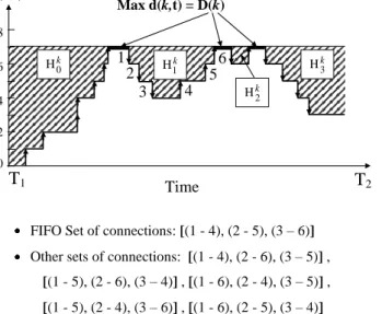
The chain-extraction procedure allows an arrival-departure connection for any pair within a given hollow (on each DF). The pairs considered are deleted, and the procedure continues. Figure 1 illustrates one DF atk. This d(k,t)has four hollows,
Hjk, j=0,1,2,3, withH1khaving arrivals of Trips 1, 2, and 3 and departures of Trips 4, 5, and 6. Below Figure 1 are the FIFO connections (within this hollow) as well as other alternatives; in all, the minimum fleet size atk, D(k), is maintained.
Max d(k,t) = D(k) 1 2 3 4 6 5 8 6 4 2 0
T
1 TimeT
2FIFO Set of connections: [(1 - 4), (2 - 5), (3 – 6)]
Other sets of connections: [(1 - 4), (2 - 6), (3 – 5)] ,
[(1 - 5), (2 - 6), (3 – 4)] , [(1 - 6), (2 - 4), (3 – 5)] , [(1 - 5), (2 - 4), (3 – 6)] , [(1 - 6), (2 - 5), (3 – 4)] k 0 H k 1 H k 2 H k 3 H d(k,t)
Fig. 1.Example of creating trips connections within one hollow,H1k, using the FIFO rule and all other possibilities while maintaining the minimum fleet size attained
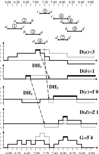
A nine-trip example with four terminals(a, b, c,andd) is presented in Table 1 and Figure 2; Table 1 shows the data required for this simple example.
Table 1.Input data for the problem illustrated in Figure 2
Trip No. Departure Terminal Departure Time Arrival Terminal Arrival Time Deadheading (DH) Trips Between Terminals DH Time (same for both
directions) 1 a 06:00 c 06:30 a – b 20 min 2 a 06:20 b 06:50 3 b 06:40 a 07:10 a – c 10 min 4 a 07:00 a 07:20 5 c 07:10 a 07:30 a – d 60 min 6 c 07:40 a 08:10 7 d 07:50 d 08:10 b – c 30 min 8 d 08:00 c 08:30 9 b 08:30 d 09:00 b – d 30 min c - d 20 min
Four DFs are constructed along with the overall DF. According to the NT proce-dure, terminald(whose first hollow is the longest) is selected for a possible reduction in D(d). The DH-insertion process continues using the criterion R=2. The first UR-DHC is DH1+DH2, and the second DH3. The result is that D(c) and D(d) are reduced from 1 to 0 and from 2 to 1, respectively; hence, N = D(S) = 5, and G is increased from 3 to 4 using three inserted DH trips. The five FIFO-based blocks are as follows: [1-5-DH2-9],[2-DH1-7],[3-DH3-6],[4],[8]. . b c c a a d a a a a b a d 2 6 5 1 3 4 7 c d b 9 c d 8 Fixed Schedule
d(
a
,t)
d(
b
,t)
D(
a
)=3
d(
d
,t)
4 3 2 1 0D(
b
)=1
3 2 1 0d(
c
,t)
3 2 1 0 -1 3 2 1 0 -1g(t)
4 3 2 1 0 6:00 6:20 6:40 7:00 7:20 7:40 8:00 8:20 8:40 9:00 Time 6:00 6:20 6:40 7:00 7:20 7:40 8:00 8:20 8:40 9:00 TimeG=3 4
D(
d
)=2 1
D(
c
)=1 0
DH
2DH
3DH
12.3.
Variable scheduling
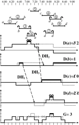
A small amount of shifting in scheduled departure times becomes almost common in practice when attempting to minimize fleet size or the number of vehicles required. However, the transit scheduler who employs shifting in trip-departure times is not al-ways aware of the consequences that could arise from these shifts. Ceder (2003, 2007b) presented methods, mostly according to the DF, to realize a variable trip schedule in an efficient manner.
Let [ti-∆i(−), ti+∆i(+)] be the tolerance time interval of the departure time of trip i, in which:∆i(−)= maximum advance of the trip’s scheduled departure time (the case of an early departure), and ∆i(+)= maximum delay from the scheduled departure time (the case of a late departure).
b c c a a d a a a a b a d 2 6 5 1 3 4 7 c d b 9 c d 8 Fixed Schedule d(a,t) d(b,t) D(a)=3 2 d(d,t) 4 3 2 1 0 D(b)=1 3 2 1 0 d(c,t) 3 2 1 0 -1 3 2 1 0 -1 g(t) 4 3 2 1 0 6:00 6:20 6:40 7:00 7:20 7:40 8:00 8:20 8:40 9:00 Time 6:00 6:20 6:40 7:00 7:20 7:40 8:00 8:20 8:40 9:00 Time G= 3 D(d)=2 1 0 D(c)=1 0 DH2 DH3 DH1
Fig. 3.The nine-trip example (of Figure 2), first with shifting and second with DH trip insertion, for reducing fleet size
The nine-trip example illustrated in Figure 2 is used for possible shifting depar-ture times in Figure 3, which employs the DF display. The tolerances of this example are∆i(+)=∆i(−)=5minutes for all trips in the schedule. Starting with shifting Trip 3 backward and Trip 4 forward by 5 minutes results in reducing D(a) from 3 to 2. This may be continued with shifting Trips 7 and 8 to reduce D(d) from 2 to 1.
Because no further shifting in departure times is feasible for the given tolerances, the process becomes one of searching for URDHC using DH trip insertion. This yields three DH trips resulting in Min N = G (Snew) = metricconverterProductID3, in3, in which Snewis the new schedule. The three blocks are determined by FIFO:[1-5-DH2 -9],[2-DH1-7-8], and[3-4-DH3-6]. In case a DH trip insertion is not allowed, the shift-ing process will end with Min N = 5 and the FIFO-based blocks:[1-5],[2-9],[3-4], [7-8],[9].
3.
Vehicle-chain construction using crew-cost approach
There are two predominant characteristics in transit-operations planning: (a) differ-ent resource requiremdiffer-ents between peak and off-peak periods, and (b) working dur-ing irregular hours. These characteristics result in split duties (shifts) with unpaid in-between periods. Often it called swing time. The inconvenience accompanying split duties led driver (crew) unions to negotiate for an extension of the maximum allowed driver’s idle time for which the driver can still get paid. It is common, therefore, to have a constraint in a labor union agreement specifying this maximum paid idle time (swing time), to be termed Tmax.
The crew-scheduling problem from the agency’s perspective is known to be the minimum crew-cost problem. With this minimum-cost orientation in mind, the DF (deficit function) properties can be used to construct vehicle chains (blocks) that take into account Tmax.In other words, to maximize idle times (swing times) that are larger than Tmax, and hence to reduce crew costs.
3.1.
Arrival-departure joinings within hollows
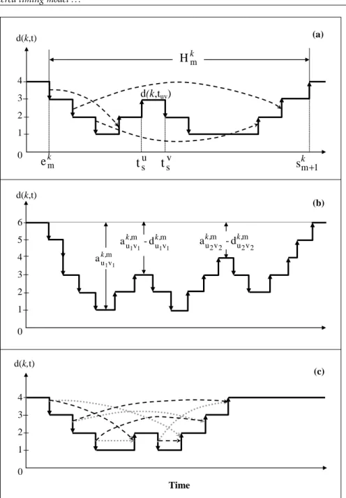
The following description uses the notation and definitions associated with the DFs. Each hollow of a DF, d(k,t) at terminalk, contains the same number of departures and arrivals, except for the first and last hollow at the beginning and end of the schedule horizon. This is due to the fact that each arrival reduces d(k,t) by one and each depar-ture increases it by one, so that the hollow starts and ends at D(k).
For a given hollow,Hmk, letImk be the set of all arrival epochstieinHmk, and letJmk be the set of all departure epochstjsinHmk. The difference in time between departure and arrival is defined as∆ij = tjs−tiefort
j
s > tieinHmk. The joining (connection) betweentieandt
j
sin a vehicle block is effectively the idle time between trips; hence, ∆ijmay represent this idle time. In addition a local peakuvis defined within hollow Hmk as d(k,tuv) betweentus and tve in which ekm < tus ¬ tuv ¬ tve < skm+1, where
Hk
of a local peak,uv, has more than one departure or arrival, then it suffices to refer to only one of them (asuorv). Letdkuv,mbe the number of departures inHmk before and includingtus, anda
k,m
uv be the number of arrivals inHmk beforetus.
Lemma 1. The number of arrival-departure joinings in hollowHmk beforetusmust bedkuv,m.
Proof. If some departure epochs before a local peak, uv, are left without a joining, it will be impossible to connect them with arrival epochs aftertve. That is, each departure epoch before and includingtus must have a joining to an earlier arrival time within Hmk. This can be seen in Figure 4(a).
Lemma 2. The number of arrival-departure joinings that can be constructed aftertvewithin
Hmk isakuv,m−dkuv,m
.
Proof. Given hollowHmk and local peakuv, then based onLemma 1and the charac-teristics of local peaks in hollows,dkuv,m, departure epochs must and can be joined to earlier arrival epochs inHmk; hence, the number of arrival epochs left over without joinings is
akuv,m−dkuv,m
for all local peaks. Figure 4(b) displays this explanation.
Lemma 3. The sum of all idle times within any hollow is a fixed number and independent of
any procedure aimed at joining arrival and departure epochs; that isP
i,j∆ij = constant.
Proof. LetHmk havenarrivals andndepartures. It is noted previously that the number of departures and arrivals are the same within each middle hollow (i.e., excluding the first and last hollows). Let two different n-joining arrangements with idle times∆1ij and∆2ijfor all joinings betweeni∈Imk andj ∈Jmk be expressed as follows:
X i,j ∆1 ij = X i,j tjs1−tie1=X j tjs1−X i tie1; and similarly X i,j ∆2 ij= X j tjs2−X i tie2
d(k,t) d(k,t) d(k,t) d(k,tuv) k m
H
a umv 1 1 k , d -a umv umv 1 1 1 1 k , k , a -d m v u m v u2 2 2 2 k , k , k me
t
sut
vss
km 1 Time (c) (b) (a) 4 3 2 1 0 6 5 4 3 2 1 0 4 3 2 1 0Fig. 4.Part (a) describes examples of arrival-departure joining to support Lemma 1; part (b) interprets Lemma 2; part (c) shows two 4-joining examples of Lemma 3
It is known that the sum of all departure or arrival times in a hollow is a fixed number; hencePi,j∆1ij=
P
i,j∆2ij = constant. Figure 4(c) further clarifies this argu-ment.
3.2.
Objective function and formulation
In constructing the blocks at each DF, the aim is to maximize the number of times in which∆ij Tmax; in other words, to reduce crew cost. At the same time, however, for cases in which∆ij< Tmax, from a crew’s fairness perspective, it will be reasonable to attempt to have equitable paid idle times. This was for a simple reason, to eliminate a situation in which some drivers will have long and some short paid idle times. In what follows is a formulation of the main objective and then a secondary objective.
For a given hollowHmk at terminalk, letxijbe a0−1variable associated with a trip-joining between the arrival of theithtrip toHmk and the departure fromHmk of thejth. The problem of finding the maximum number of idle times greater than or equal toTmaxin hollowHmk is as follows:
Problem P1. M axZ4= X i∈Ikm X j∈Jkm xij (2) Subject to: X j∈Jk m xij¬1, i∈Ikm (3) X i∈Ik m xij¬1, j∈Jmk (4) xij={0, 1}, i∈Ikm, j∈Jmk (5)
The binary decision variables are determined by:
xij = 1, tjs−tieTmax 0, otherwise
A solution with xij=1 indicates that joining trips i (arrival epoch) and j (depar-ture epoch) results in an idle time larger than or equal Tmax. Constraints (3) and (4) insure that each trip inHmk may be joined with, at most, one successor trip, and one predecessor trip, respectively.
Trips that were not joined in the solution of P1 are subject to a secondary objec-tive: equitable paid idle times. It is shown below that joinings with this secondary objective are based on the FIFO rule. Balancing∆ijfor∆ij<Tmaxis the same as mini-mizing the difference between each∆ijand its average∆¯ijeither by absolute difference or by least-square difference. The FIFO rule used for this balancing is stated in the fol-lowing theorem.
Theorem 1. Minimizing the least-square differences between∆¯ijand each∆ijfor alli∈Imk
andj∈JmkinHukis accomplished by constructing joinings using the FIFO rule.
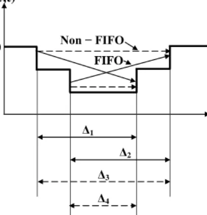
Proof. It is sufficient to prove Theorem 1 on a simple, but generalized example, as illustrated in Figure 5, with a hollow containing two arrivals and two departures.
i i
“tlm2011” — 2012/11/20 — 13:53 — page 35 — #35
i i
Two tiered timing model . . . 35
t Δ1 Δ2 Δ3 Δ4 d(k,t) D(k) Non − FIFO FIFO
Fig. 5.Example of a comparison of joinings based on FIFO and other rules
It may be shown that ∆1−∆ 2 + ∆2−∆ 2 < ∆3−∆ 2 + ∆4−∆ 2 (6) where∆is the average arrivdeparture joining length in the example. Using an al-gebraic expression, then (6) becomes
∆2
1+∆22−∆23−∆24<2∆(∆1+∆2−∆3−∆4) (7) Lemma 3states that∆1+∆2 =∆3+∆4, and hence the right-hand side of expression (7) is zero. FromLemma 3one can further obtain(∆1+∆2)2 = (∆3+∆4)2or∆21+ ∆2
2−∆23−∆24=2∆3∆4−2∆1∆2. The latter is inserted into (7) to yield
∆3∆4<∆1∆2 (8)
Based, again, onLemma 3, let∆3−∆1=∆2−∆4=Bor∆1=∆3−Band∆4=∆2−
B; these last two equations are inserted into (8) to obtain∆3(∆2−B)<∆2(∆3−B), which yields∆3>∆2. The last result must be correct from Figure 5, and therefore it agrees with expression (6).
4.
Maximum unpaid idle times
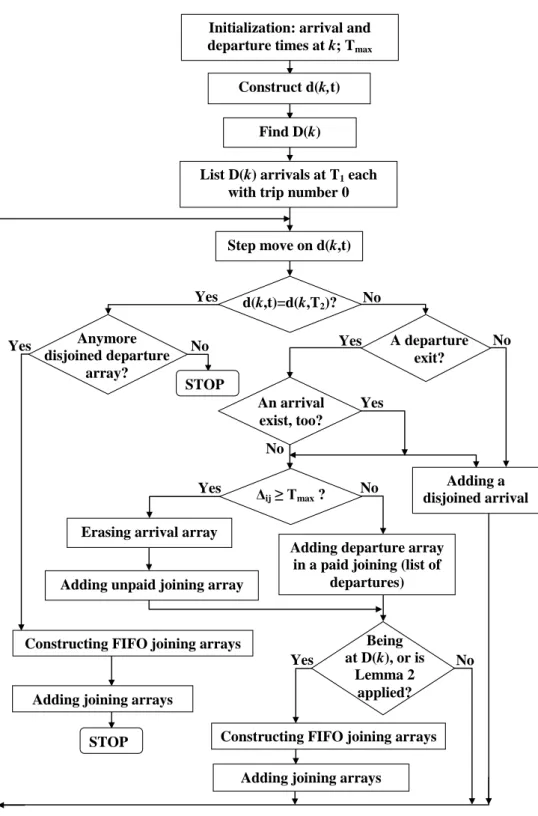
The mathematical programming formulation in Equations (2)–(5) is aimed at max-imizing the number of idle times that are longer than or equal to Tmax. However, this formulation may involve a very large number of computations (NP-Complete), hence entailing the use of another (more simplified) procedure. Such a procedure is described in a flow diagram in Figure 6 and contains both Tmaxand FIFO rule con-siderations; the latter is for joining arrivals and departures with paid idle times. Let us call this procedure algorithm TmF.
d(k,t)=d(k,T2)? A departure exit? Anymore disjoined departure array? Adding a disjoined arrival array Adding departure array
in a paid joining (list of departures) Erasing arrival array
Adding unpaid joining array
Constructing FIFO joining arrays
Adding joining arrays
Constructing FIFO joining arrays Adding joining arrays
STOP
STOP
Initialization: arrival and departure times at k; Tmax
Construct d(k,t)
Find D(k)
List D(k) arrivals at T1 each
with trip number 0
Step move on d(k,t) An arrival exist, too? Yes Yes Yes Yes Yes Yes No No No Being at D(k), or is Lemma 2 applied? No No No Δij ≥ Tmax ?
The input for algorithm TmF for each terminalkconsists of two arrays, the arrival and departure arrays, and a given Tmax. This input enables constructing DF atkand obtaining D(k) following the insertion of DH trips and the shifting of departure times for minimizing fleet size (see Section 2). Because D(k) vehicles are required atk, we assume their arrivals there to be at (or before) T1( the start of the schedule horizon). Algorithm TmF moves by steps on d(k,t), in which each step refers to a change in d(k,t) or the detection of a dot on d(k,t); the dot means that arrival and departure epochs at koverlapped att.
Algorithm TmF continues with a check of the end of the schedule horizon and detects the nature of the change (or dot) in d(k,t). For each departure epoch,∆ij is examined to determine whether it is greater than or equal to Tmax; if greater, then an unpaid joining array is added, otherwise a disjoined departure time array is added. Each arrival epoch (detected in a step move in Figure 6) is added as a disjoined arrival array. If a departure epoch is identified in a step move, the algorithm looks for a possible dot on d(k,t), adding its arrival epoch to the list of disjoined arrival arrays. At the end of the process, the algorithm constructs joining arrays from the disjoined arrival and departure arrays, using the FIFO rule. The complete process is shown in Figure 6.
5.
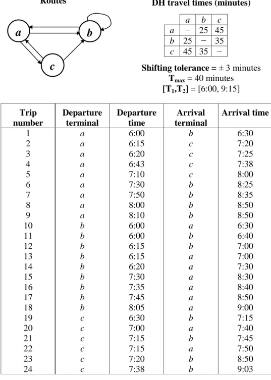
Real-life examples
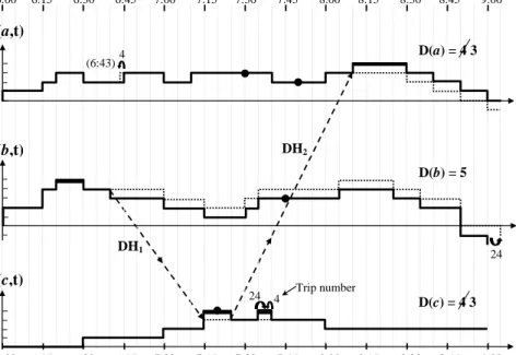
An example of constructing vehicle chains (blocks), including the employment of algorithm TmF, is shown in Figures 7–9. This example is based on real-life schedul-ing data from EGGED the large national bus carrier of Israel. The example, consist-ing of three terminals and a 24-trip schedule, is exhibited in Figure 7, includconsist-ing DH travel time matrix, shifting tolerance, Tmax, and schedule horizon. It should be noted, though, that DH travel time between terminalsbandcis considered in both directions although there is only a service route between c and b. The fleet-reduction procedure, involving the shifting of departure times and DH trip insertions, is shown in Figure 3; here it is applied to the example of Figure 7 in Figure 8. Two DH trips and two shifts are introduced into the process to reduce D(a) and D(c) from four to three, resulting in a fleet size of eleven vehicles. The shifts are shown in Figure 8 by their shifting length and trip number. It can be seen from this Figure that the only middle hollow containing more than a single departure is the second hollow of d(b,t); hence, only this hollow is subject to the process of algorithm TmF.
Figure 9(a) describes the solution for algorithm TmF in comparison with a so-lution based only on the FIFO rule in Figure 9(b). The trip numbers of the example, appearing in Figure 7 are added to Figure 9. AlgorithmTmF results in two unpaid joinings between the arrivals of trips 11 and 12 and the departures of trips 15 and 17, respectively. In both cases,∆ij >Tmax = 40 minutes. The remaining joinings in Figure 9(a) are based on the FIFO rule. The use of only the FIFO rule for the entire process results in only one unpaid joining (that between trips 11 and 15) as is shown in Figure 9(b).
DH travel times (minutes)
a
b
c
a
− 25 45
b
25 − 35
c
45 35 −
Shifting tolerance =
± 3 minutes
T
max= 40 minutes
[T
1,T
2]
= [6:00, 9:15]
Trip
number
Departure
terminal
Departure
time
Arrival
terminal
Arrival time
1
2
3
4
5
6
7
8
9
10
11
12
13
14
15
16
17
18
19
20
21
22
23
24
a
a
a
a
a
a
a
a
a
b
b
b
b
b
b
b
b
b
c
c
c
c
c
c
6:00
6:15
6:20
6:43
7:10
7:30
7:50
8:00
8:10
6:00
6:00
6:15
6:15
6:20
7:30
7:35
7:45
8:05
6:30
7:00
7:15
7:15
7:20
7:38
b
c
c
c
c
b
b
b
b
a
b
b
a
a
a
a
a
a
b
a
b
a
b
b
6:30
7:20
7:25
7:38
8:00
8:25
8:35
8:50
8:50
6:30
6:40
7:00
7:00
7:30
8:30
8:40
8:50
9:00
7:15
7:40
7:45
7:50
8:50
9:03
Routes
a
b
c
Fig. 7.Example consisting of 24 trips and 3 terminals for constructing vehicle chains with the Tmax
(6:43) 4 d(b,t) 24 DH1 DH2 D(b) = 5 d(c,t) 6:00 6:15 6:30 6:45 7:00 7:15 7:30 7:45 8:00 8:15 8:30 8:45 9:00 Time D(c) = 4 3 24 4 6:00 6:15 6:30 6:45 7:00 7:15 7:30 7:45 8:00 8:15 8:30 8:45 9:00 Time d(a,t) Trip number D(a) = 4 3 4 2 0 4 2 0 4 2 0
Fig. 8.The 24-trip example (depicted by three DFs) undergoing a DH trip-insertion procedure, combined with shifting departure times
(a) Joining based on TmF
Time
(b) Joining based on FIFO
d(b,t) 6:00 6:30 7:00 7:30 8:00 8:30 9:00 10 11 12 13 14 1 11 12 19 15 16 21 17 18 6 7 8 9 23 24 DH1 d(b,t) 6:00 6:30 7:00 7:30 8:00 8:30 9:00 10 11 12 13 14 1 11 12 19 15 16 21 17 18 6 7 8 9 23 24 DH1 4 2 0 4 2 0 D(k) = 5 D(k) = 5 Trip number
Fig. 9.Arrival-departure joinings for constructing vehicle chains (blocks) in the middle hollow of terminal b, utilizing in (a) the TmF algorithm, and in (b) the FIFO rule
The final phase of the arrival-departure joining process is to construct vehicle blocks. This will contain the joinings created and other FIFO-based joinings in order to make a complete set of blocks. The eleven blocks of the 24-trip-schedule example, based on algorithm TmF (at terminalb), are given by their numbers in the following list:[1-DH1-22-7],[10-4-24], [11-15],[2-23], [12-17],[13-5],[3-DH2-9],[14-6],[19-16], [20-8],[21-18]. The process based only on the FIFO rule results in the same blocks, except for the 5thand 9thblocks, which become[12-16]and[19-17], respectively.
Finally it is worth noting that the idea presented turned to be very useful in practice. It allows the scheduler to do things both manually and automatically. In addition of using this idea in the EGGED bus carrier, with about 3000 buses, it was implemented by the large KMB bus company in Hong Kong with about 4000 buses. In both cases this implementation resulted in a significant cost reduction.
6.
Concluding remark
The criteria for transit crew scheduling are based on an efficient use of manpower re-sources while maintaining the integrity of any work-rule agreements. The construc-tion of the selected crew schedule is usually a result of the following sub-funcconstruc-tions: (i) duty piece analysis; (ii) work-rules coordination; (iii) feasible duty construction; and (iv) duty selection. The duty-piece analysis partitions each vehicle block at selected relief points into a set of duty pieces. These duty pieces are assembled in a feasible duty-construction function. Other required information: travel times between relief points and a list of relief points designated as required duty stops and start locations. The focus of this work is related indirectly to the assembling of duty pieces using a practical minimum-cost approach in the process of constructing vehicle schedules.
From the transit agency’s perspective, the largest single cost item in the budget is the driver’s wage and fringe benefits. Because of the important implications of crew scheduling for providing good transit service, practitioners ought to comprehend the root of the problem, and be equipped with basic tools to be able to arrive at a solution. This work provides a useful tool using the characteristics of split crew duties (shifts) with unpaid in-between periods; these split duties are the result of different resource requirements between peak and off-peak periods. The analysis presented provides an optimal solution for maximizing the unpaid shift periods, hence reducing the crew costs, with the assurance of maintaining the minimum number of vehicles required.
References
[1] Banihashemi, M. and Haghani, A., (2000). Optimization model for large-scale bus transit
scheduling problems. Transportation Research Record, 1733, pp. 23–30
[2] Beasley, J. E. and Cao, E. B., (1996).A tree search algorithm for the crew scheduling problem. European Journal of Operational Research, 94, pp. 517–526
[3] Beasley, J. E. and Cao, E. B., (1998).A dynamic programming based algorithm for the crew
[4] Borndorfer, R., Lobel, A., and Weider, S., (2008).A Bundle Method for Integrated Multi-Depot
Vehicle and Duty Scheduling in Public Transit. Computer-Aided Systems in Public Transport (M. Hickman, P. Mirchandani, S. Voss, eds). Lecture notes in economics and mathematical systems, Vol. 600, Springer, pp. 3–24
[5] Carraresi, P., Nonato, M., and Girard, L., (1995).Network models, lagrangean relaxation
and subgradients bundle approach in crew scheduling problems. In Computer-aided Transit Scheduling. Lecture Notes in Economics and Mathematical Systems, 430 (J. R. Daduna, I. Branco, and J. M. P. Paixao, eds.), pp. 188–212, Springer-Verlag
[6] Ceder, A., (2002)A step function for improving transit operations planning using fixed and
vari-able scheduling, in Transportation and Traffic Theory, M.A.P. Taylor, (ed), pp. 1–21, Elsevier Science
[7] Ceder, A., (2003).Public transport timetabling and vehicle scheduling. Chapter 2 in Advanced Modeling for Transit Operations and Service Planning (W. Lam and M. Bell, eds.), pp 31–57, Pergamon Imprint, Elsevier Science
[8] Ceder, A., (2007a).Optimal Single-Route Transit Scheduling. Transportation & Traffic The-ory (R. Allsop, M. Bell, B. Heydecker, eds), ISTTT-17, Elsevier Science & Pergamon Pub., pp. 385–405
[9] Ceder, A., (2007b).Public Transit Planning and Operation: Theory, Modeling and Practice, El-sevier, Butterworth-Heinemann, Oxford, UK, 640 p.
[10] Ceder, A. and Stern, H.I., (1981).Deficit function bus scheduling with deadheading trip
inser-tion for fleet size reducinser-tion. Transportation Science, 15 (4), pp. 338–363
[11] Clement, R. and Wren, A., (1995).Greedy genetic algorithms, optimizing mutations and bus
driver scheduling. In Computer-Aided Transit Scheduling. Lecture Notes in Economics and Mathematical Systems, 430 (J. R. Daduna, I. Branco, and J. M. P. Paixao, eds.), pp. 213–235, Springer-Verlag
[12] Fores, S., Proll, L., and Wren, A., (1999).An improved ILP system for driver scheduling. In Computer-Aided Transit Scheduling. Lecture Notes in Economics and Mathematical Sys-tems, 471 (N. H. M. Wilson, ed.), pp. 43–61, Springer-Verlag
[13] Fores, S., Proll, L., and Wren, A., (2001). Experiences with a flexible driver scheduler. In Computer-Aided Scheduling of Public Transport. Lecture Notes in Economics and Math-ematical Systems, 505 (S. Voss and J. R. Daduna, eds.), pp. 137–152, Springer-Verlag [14] Freling, R., Huisman, D., and Wagelmans, A. P. M., (2001). Applying an integrated
ap-proach to vehicle and crew scheduling in practice. In Computer-Aided Scheduling of Public Transport. Lecture Notes in Economics and Mathematical Systems, 505 (S. Voss and J. R. Daduna, eds.), pp. 73–90, Springer-Verlag.
[15] Gertsbach, I. and Gurevich, Y., (1977).Constructing an optimal fleet for transportation
sched-ule. Transportation Science, 11, pp. 20–36
[16] Gintner, V., Kliewer, N. and Suhl, L., (2008).A Crew Scheduling Approach for Public Transit
Enhanced with Aspects from Vehicle Scheduling. Computer-Aided Systems in Public Trans-port (M. Hickman, P. Mirchandani, S. Voss, eds). Lecture notes in economics and mathe-matical systems, Vol. 600, Springer, pp. 25–42
[17] Haase, K., Desaulniers, G., and Desrosiers, J., (2001).Simultaneous vehicle and crew
[18] Haghani, A. and Banihashemo, M., (2002).Heuristic approaches for solving large-scale bus
transit vehicle scheduling problem with route time constraints. Transportation Research, 36A, pp. 309–333
[19] Haghani, A., Banihashemi, M., and Chiang, K. H., (2003).A comparative analysis of bus
transit vehicle scheduling models. Transportation Research, 37B, pp. 301–322
[20] Huisman, D., Freling, R., and Wagelmans, A.O.M., (2004).A robust solution approach to the
dynamic vehicle scheduling problem. Transportation Science, 38 (4), pp. 447–458
[21] Huisman, D., Freling, R., and Wagelmans, A. P. M., (2005).Models and algorithms for
inte-gration of vehicle and crew scheduling. Transportation Science, 39, pp. 491–502
[22] Kroon, L. and Fischetti M., (2001).Crew scheduling for Netherlands railways “destination:
cus-tomer.”In Computer-Aided Scheduling of Public Transport. Lecture Notes in Economics and Mathematical Systems, 505 (S. Voss and J. R. Daduna, eds.), pp. 181–201, Springer-Verlag
[23] Kwan, A. S. K., Kwan R. S. K., and Wren, A., (1999).Driver scheduling using genetic
algo-rithms with embedded combinatorial traits. In Computer-Aided Transit Scheduling. Lecture Notes in Economics and Mathematical Systems, 471 (N. H. M. Wilson, ed.), pp. 81–102, Springer-Verlag
[24] Kwan R.S.K and Kwan A.S.K., (2007).Effective Search Space Control for Large and/or Complex
Driver Scheduling Problems. Annals of Operations Research 155, pp. 417–435
[25] Laplagne, I., Kwan R.S.K., and Kwan A.S.K., (2009).Critical Time Window Train Driver Relief
Opportunities. Public Transport planning and Operations 1(1), pp. 73–85
[26] L ¨obel, A., (1998),Vehicle scheduling in public transit and lagrangean pricing. Management Science, 44 (12), pp. 1637–1649
[27] L ¨obel, A., (1999).Solving large-scale multiple-depot vehicle scheduling problems. In Computer-Aided Transit Scheduling. Lecture Notes in Economics and Mathematical Systems, 471 (N. H. M. Wilson, ed.), pp. 193–220, Springer-Verlag
[28] Lourenco, H. R., Paixao, J. P., and Portugal, R., (2001).Multiobjective metaheuristics for the
bus-driver scheduling problem, Transportation Science, 35(3), pp. 331–343
[29] Mesquita, M. and Paixao, J.M.P., (1999).Exact algorithms for the multi-depot vehicle scheduling
problem based on multicommodity network flow type formulations. In Computer-Aided Tran-sit Scheduling. Lecture Notes in Economics and Mathematical Systems, 471 (N. H. M. Wilson, ed.), pp. 221–243, Springer-Verlag
[30] Mesquita, M., Paias, A., and Respicio, A., (2009).Branching Approaches for Integrated Vehicle
and Crew Scheduling. Public Transport Planning and Operations 1(1), pp. 21–37
[31] Mingozzi, A., Boschetti, M. A., Ricciardelli, S, and Bianco, L., (1999).A set partitioning
approach to the crew scheduling problem. Operations Research, 47, pp. 873–888
[32] Paias, A. and Paixao, J.M.P., (1993).State space relaxation for set-covering problems related to
bus driver scheduling. European Journal of Operational Research, 71, pp. 303–316 [33] Shen, Y. and R. S. K. Kwan., (2001).Tabu search for driver scheduling. In Computer-Aided
Scheduling of Public Transport. Lecture Notes in Economics and Mathematical Systems, 505 (S. Voss and J. R. Daduna, eds.), pp. 121–135, Springer-Verlag
[34] Stern, H.I. and Ceder, A., (1983).An improved lower bound to the minimum fleet size problem. Transportation Science, 17 (4), pp. 471–477