Computer Interfaces
J. Asensio-Cubero1, J. Q. Gan1and R. Palaniappan2
1University of Essex,Wivenhoe Park, Colchester, Essex CO4 3SQ,United Kingdom 2University of Wolverhampton, Shifnal Road, Telford, TF2 9NT, United Kingdom
E-mail:[email protected],[email protected],[email protected]
Abstract. Objective:Multiresolution analysis (MRA) offers a useful framework for signal analysis in the temporal and spectral domains, although commonly employed MRA methods such as Daubechies wavelets may not be the best approach for brain computer interface (BCI) applications. Approach: Hereby we propose the use of a lifting scheme transform over graphs and a tailored simple graph representation for EEG data which results on a MRA system where temporal, spectral and spatial characteristics are used to extract motor imagery features. The transformed data is processed within a simple experimental framework to test the classification performance.Main Results:The proposed method can significantly improve the classification results obtained by various wavelet families using the same methodology. Preliminary results using common spatial patterns as feature extraction method show that we can achieve comparable classification accuracy to more sophisticated methodologies. From the analysis of the results we can obtain insights into the pattern development in the EEG data, which provide useful information for feature basis selection and thus for improving classification performance. Significance: Applying wavelet lifting over graphs is a new approach for handling BCI data. The inherent flexibility of the lifting scheme could lead to new approaches based on the proposed method which could further improve the classification performance here presented.
1. Introduction
Brain computer interfaces (BCI) are control systems that make use of the cognitive states of the user to operate a computer or similar device [1]. Although the idea was introduced more than 30 years ago [2], the field has rapidly grown during the last decade and a half. BCIs not only have a direct positive impact on users with disabilities in terms of quality of life and communication with their environment, but also offer new modes of human machine interaction for both disabled and healthy users.
Electroencephalography (EEG) is the signal acquisition technique for many BCI systems. EEG equipment is inexpensive compared to other technologies such as functional magnetic resonance imaging (fMRI) and, as it is a non-intrusive method, no surgical procedure is required to place the electrodes (unlike methods based on electrocorticogram (ECoG)).
In this study, we focus on a BCI paradigm known as Motor Imagery (MI). Limb movement imagination provokes a series of short lasting amplifications and attenuations in the EEG data known as event related desynchronisation (ERD) and event related synchronisation (ERS) [3]. ERD/ERS analysis has proven to be a complex task as it occurs in different parts of the cortex, at different frequencies, and during different time intervals. Furthermore, as EEG data is often of low amplitude and noisy, there is no consistency in the patterns among
different subjects, and worse still, the arising patterns can change within a session for the same subject. In many instances, researchers have used wavelet decompositions to study the EEG data behaviour due to their temporal-spectral capabilities.
Wavelets, or first generation wavelets (FGWs), offer a multi-resolution analysis (MRA) framework [4] where the signal is represented using small blocks (shiftings and dilations of the wavelet functionψat different resolutions), obtaining a more compact representation in both time and frequency domains. FGWs need a specificψfunction that is suitable to the domain of application. Therefore, different wavelet families are designed for different applications. Constructing an ad-hoc wavelet family for specific needs is far from easy, this is the reason why researchers commonly utilise well studied families such as Daubechies or Coifflets.
Wavelet lifting, known as the second generation wavelets, offers a new approach to MRA where the steps to build new wavelets are more straightforward. Another inherent advantage of the lifting scheme is the low resource consumption, as it can be calculated in-place. FGWs can also be implemented within the lifting scheme framework [5] considerably speeding up their performance. Several studies in the BCI field have taken advantage of this property [6] [7]. Wavelet lifting can be also applied in domains where the Fourier transform does not exist, such as unevenly sampled data, functions defined over surfaces and graphs [8], the latter being highly interesting.
In this study, we propose a new lifting scheme (LS) that can cope with the three domains involved in the ERS/ERD analysis (temporal, spectral and spatial domains). An MI trial can be represented as a fully connected simple graph where the nodes are the readings of the electrodes at a given instant. Therefore, an appropriately designed LS should be able to extract the temporal-spatial information, inherent in the graph representation, combined with the temporal-spectral features extracted during the MRA process. This concept can be also expanded to other BCI paradigms.
To the authors’ knowledge, the study here applies LS over graphs for the first time in the BCI domain, which is not only suitable for EEG data analysis, but also opens new avenues due to its flexible nature. The paper is organised as follows. The data acquisition is detailed in Section 2.1, Section 2.2 explains the lifting scheme over graphs, Section 2.3 describes the simple graph representation used on EEG data, Section 2.4 focuses on the feature extraction technique and pattern description, classification methods are covered in Section 2.5, and the experimental methodology is described in Section 2.6. The results obtained along with discussions are presented in Section 3. Finally, the conclusions are drawn in Section 4. 2. Methods
2.1. Data Acquisition
Two different data sets were used in this study. The first one was recorded in the BCI Laboratory at the University of Essex. The second dataset was obtained from the BCI Competition IV (dataset 2a) [9].
The Essex dataset (subjects prefixed withE-in the data analysis) contained three different classes: imaginary movements of right hand, left hand and feet. There were 12 healthy subjects: 58% female, 50% naive to BCI, and ages ranging from 24 to 50. The subjects sat in an arm-chair facing a computer screen, with 32 electrodes placed on the scalp following the extension of the 10-20 international location system. Initially, att= 0s, a fixation cross was printed on the screen, after two seconds (att= 2s) a cue was shown indicating the imaginary movement class to perform. The fixation cross and cue disappeared att= 8sindicating the end of the trial. The EEG data was recorded with a sampling frequency of 256 Hz during four
Figure 1. Numbering of the 15 electrodes used during the experimentation, which were allocated from FC3 to FC4, C3 to C4, and CP3 to CP4.
different runs, producing a total of 120 trials for each class.
The competition dataset (subjects prefixed withC-) contained four classes of imagined movement data: right-hand, left-hand, feet and tongue. From the available details found in [10] we know that eight of the nine subjects had an average age of23.8±2.5years, 37.5% were female, and all of them were BCI naive subjects. No information is provided regarding the ninth subject. The acquisition protocol was similar to the one used for the Essex dataset and it is fully explained in [11]. In this case, 22 channels were recorded with a sampling frequency of250Hz. During each of the two sessions, a total of 288 trials were recorded per subject.
For both datasets, we only use the channel subset as shown in Figure 1, which covers the major area of the motor cortex.
For experimental purposes both datasets were split into training and evaluation subsets. In the Essex dataset, the data from the first two runs were dedicated to training (180 trials), and the last two runs were used for evaluation (180 trials). The competition dataset was already evenly divided into two subsets, each with 288 trials.
2.2. Wavelet lifting over graphs
A multiresolution analysis system consists of a sequence of successive approximation spaces which obey a series of constraints to assure an approximation that is as close as required to the original signal [4] [12]. From the application point of view, such systems are highly useful as the analysed signals present different characteristics at different decomposition levels.
The discrete wavelet transform (DWT) is a specific example of an MRA system and it is defined as an addition of two different coefficient sets [13], which are related to the mother wavelet functionψ[n]and the father wavelet functionφ[n]:
x[n] =al0[n] + l0 X l=0 dl[n] al0[n] = 2l0−1 X k=0 Sl0,kφl0,k[n]
dl[n] =
2l0−1 X
k=0
Tl,kψl,k[n] (1)
Equation(1) shows the decomposition of the signalx[n]until the levell0. On one hand,
al0[n] corresponds to the father wavelet projection (approximation) of the original signal
onto the level l0. On the other hand, dl[n] defines the detail coefficients for every level
l. The equation shows how the detail coefficients are related to the approximation error. Due to the orthogonal nature ofdl[n], this calculation is relatively straightforward at every level of the decomposition. The elementsSl0,k andTl,k are the projection weights onto the different subspaces computed fork= 0. . .2l0−1. The continuous wavelet transform (CWT)
is analogously defined in the continuous domain.
Different mother wavelet functions (and their complementary father function) define what are known as wavelet families. Each family (such as Daubechies, Coifflets and Morlet) is designed with a specific purpose and has particular properties.
Due to their temporal-spectral capabilities, both discrete and continuous wavelet transforms have been extensively used in the BCI domain. The most common approach is to decompose the signal into a certain level taking into account which frequencies are suitable for the desired application, followed by a feature extraction process on the different coefficient sets. In [14], a P-300 based BCI was proposed using descriptive statistics from the different levels of a CWT. This scheme is also typical in motor imagery BCIs, as in [15] where a DWT was used in the same manner.
It is also common to find other studies in which wavelet-packets were employed [16]. Due to the large number of coefficient sets obtained from the decomposition, it is typical to perform a basis selection following the coefficient calculation. Some authors perform this task by manually selecting those packets corresponding to the most relevant frequency ranges [17], although automatic techniques can also be applied [18] [19] [20].
Although wavelet analysis is a powerful tool for signal representation, it requires a strong theoretical base to develop a new family which best suits a given problem. Wavelet lifting, known as the second generation wavelets, defines a simpler process to develop MRA systems without the mathematical complexity inherent to FGW designs [21].
A lifting scheme consists of iterations of three basic operations [22]:
• Split: Divide the original unidimensional signal xof length N ∗2 into two subsets, usually referred as odd (xo) and even (xe) elements. For convenience the parity of the element index is used,xo=x[2n+ 1]andxe=x[2n]forn∈ {0. . . N−1}.
• Predict: Obtain the wavelet coefficientsdof lengthN as the error of predictingxoin base ofxeusing apredictor operatorP.
• Update: Calculate the coarser approximation of the original signalaof lengthN by combiningxeanddusing anupdate operatorU.
The forward transform function is defined as:
d=xo− P(xe)
a=xe+U(d) (2)
In order to compute the analysis until the levell0 it suffices to setxli = ali−1 after
calculating the approximation set as described in Equation (2), although it is recommended to follow the index based approach described in [22] to profit from an in-place lifting transform. It is noteworthy that the decomposition is inherently orthogonal as it is based on the approximation error.
The inverse transform function is derived from Equation (2):
xo=d+P(xe)
xe=a− U(d)
An illustrative and relevant example of a lifting scheme design based on linear interpolation is given in [22] where the predict and update functions are interpolating scaling functions:
d[n] =xo[n]−1/2(xe[n] +xe[n+ 1]) (3) In order to preserve the original signal properties we must conserve the zeroth and first moments, resulting in the following update function:
a[n] =xe[n] + 1/4(d[n] +d[n+ 1]) (4) This transform is specially suited for linear data, although it can be extended using polynomial or spline interpolation to address signals from different nature. It is also possible to implement any FGW by defining the appropriatepredictandupdatefunctions for a faster implementation than the DWT [22]. The lifting scheme is also applicable to domains where the wavelet transform does not exist such as unevenly sampled data, surfaces, manifolds or trees.
In the present study we will focus on lifting over graphs [8] which has been explored in other domains and successfully applied to video compression [23].
Consider a graphG= (V, E)whereV is the node set of sizeN =No+NeandEthe edges linking those nodes. Let us assume thatV is split into the even and odd sets andEis represented using the adjacency matrixAdj. We rearrangeV andAdj so that the odd set of nodes (a vectorVoof sizeNo×1) is gathered before the even set (a vectorVeof sizeNe×1), obtaining the following structure:
˜ V = Vo Ve ˜ Adj = F No×No JNo×Ne KNe×No LNe×Ne ! (5)
The submatricesFandLinAdj˜ in Equation (5) contain the links joining elements within the same node sets and are discarded. On the other hand, the block matrixJ contains only edges linking odd elements to even elements and, analogously,Konly links even elements to odd elements. KeepingJandKassures that we have a disjoint even/odd assignment.
The lifting transform function is then defined using the different node sets and a weighted version of the block matricesJandK:
D=Vo−Jω×Ve
A=Ve+Kω×D (6)
In Equation (6) the prediction and update functions are defined as a matrix product P = Jω×V
e andU = Kω ×D, where Jω andKω are the weighted adjacency block matrices.
The predict matrix J is weighted row-wise applying the equation Jω i,j =
1 (P
jJi,j) for each row i and column j. The weighted version of K is analogously computed as
Ki,jω = 2∗(P1
jJi,j). These weights are directly extended from Equation (3) and Equation (4) respectively.
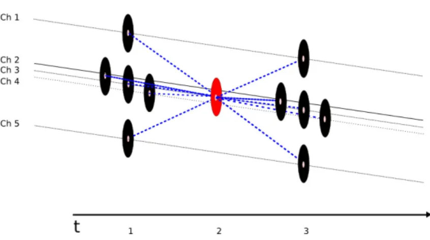
Figure 2.Details of the graph after the even/odd split. Even nodes (black circles) are used to compute the detail coefficients, approximating the odd nodes (red circles).
This weighting strategy is similar to the one originally proposed in [8], but it is specifically interesting to us as it corresponds to a discrete Laplacian filter for graphs [24], which in its simplest form is heavily used in the BCI literature.
The process described by Equation(6) is repeated on each level. For levell+ 1,V is set asAobtained in levell.
2.3. Simple graph representation for EEG data
Let us assume that an MI trialXT×CofTsamples andCchannels is contained in a simple graphGx= (Vx, Ex), whereVxdefines the nodes ( a flattened version ofX) and the edge setExis represented by an adjacency matrixAdjx:
Adji,jx =
(
1 Ifvx
i is connected tovxj
0 Otherwise (7)
The first step to build the lifting transform is to split the graph into even and odd subsets. For convenience, the odd set will correspond to the elements ofXat odd values oft, and the even set is calculated analogously. As a result, we obtain two different node vectorsvx
o and
vx e.
The adjacency submatricesKx andJxare configured such that they build a repetition of the structure as shown in Figure 2. For example, the odd nodevx
c3,t, located on the channel
c3 at instantt, is linked tovx
c3,t−1andv
x
c3,t+1as if we were applying a linear interpolation
approach. With the graph representation we also provide spatial information including the four neighbouring electrodes of the even nodevxc3,t−1: vcx1,t−1,vxc2,t−1,vxc4,t−1andvcx5,t−1; and four more neighbours ofvxc3,t+1:vcx1,t+1,vxc2,t+1,vxc4,t+1andvcx5,t+1.
This architecture is certainly not the only possible design, but it has the benefit of providing empty F and L submatrices and maintaining a channel oriented structure (obtaining the same amount of channels with the same amount of samples in every level of decomposition). Therefore, we will be able to compare this method with the results obtained from other MRA approaches.
2.4. Feature Extraction
One of the main issues in using wavelet decomposition for processing EEG is the large amount of data generated during the multi-resolution analysis. Therefore, it is always recommended to perform a feature extraction or feature reduction step. Common approaches are [20]:
• A subset of the wavelet coefficients. • Coefficient energies.
• Transformation of the coefficients by means of high order statistical methods such as principal component analysis or independent component analysis.
• Descriptive analysis of the wavelet coefficients.
In our case, we aimed to keep this step as simple as possible in order to focus on the lifting outputs, leaving a deep study of more sophisticated techniques for future research.
For every detail and approximation level we obtained 15 different sets of coefficients, one per channel, from which we computed the second moment of the coefficient distribution and applied a normalisation between 0 and 1:
fc,ld =norm(var(Dc,l))
fc,la =norm(var(Ac,l)) (8) In Equation (8)fd
c,lare the features obtained from the detail coefficients at each levell from the channelc, andfa
c,lcorresponds to the approximation coefficients.
Preliminary results indicated a superior performance by using the variance of the coefficients than other descriptive statistics or sub-band energy. Hence, this strategy was adopted.
2.5. Classification
The method used to classify the patterns from the MRA was the linear discriminant analysis (LDA). Despite its simplicity, LDA is broadly used in the BCI domain as it allows a good compromise between resource consumption and classification performance [25].
Kappa value [26] was used to measure the classification performance instead of the classification ratio. This measure gives a more accurate description of the classifier’s performance, taking into account the per class error distribution. The Kappa value was computed asκ= po−pc
1−pc , wherepois the proportion of units on which the judgement agrees (based on the output from the classifier and the actual label), andpcis the proportion of units on which the agreement is expected by chance.
2.6. Experimental Methodology
The initial step was to filter original data from 8 to 30 Hz, in order to attenuate external noise and artifacts. The filtered data was zero-centred and then each trial Xi of T samples was scaled by applyingXi= √1TXiorig(It−1t1
0
t), whereItis theT×T identity matrix and1t is aT dimensional vector with ones in it. Each trial was then segmented using a one-second window with an overlap of one fifth of a second.
The segmented data was then processed using a multi-resolution analysis approach (See Section 2.2) to the sixth level, producing twelve different coefficient sets, which were further processed to obtain the feature sets (See Section 2.4).
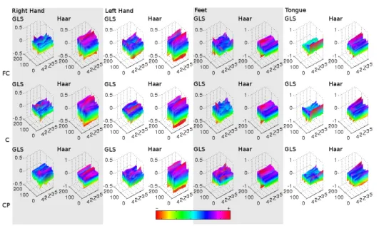
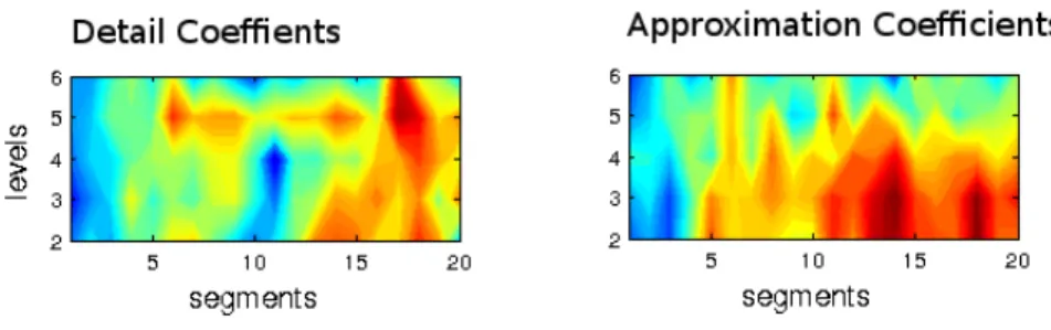
Figure 3.Average detail coefficients corresponding to the first level of decomposition for the subject C-3 using both GLS and Haar wavelets. The original segment was taken att= 4sand had a length of 256 samples. The data is split by classes so the different arising pattenrs are visible. The y axis represents the sample number and the x axis the electrode.
• Haar : Simplest FGW family related to the Daubechies family used mainly for examples in the literature.
• Db5 : Daubechies is broadly used in the BCI domain, though there does not seem to be a consensus on the filter length to use.
• Linear lifting scheme: Simplest wavelet lifting transform, frequently used as an introductory example in the literature.
• Graph lifting scheme: The newly proposed method.
The features from each level, each coefficient set (detail or approximation), and each temporal segment were classified with a separate LDA model. Therefore, for every trial to be classified, we obtained a total ofns∗l∗2LDA outputs, withnsbeing the number of segments andlthe number of levels. The final classification output for a given trial is computed as the majority voting of all the LDA outputs.
3. Results and Discussions
The first step to analyse the new MRA approach is comparing the coefficients obtained using the proposed LS method against the coefficients calculated using FGWs. Usually, the approach followed in order to give a visual comparison between two different MRAs would be to plot the decomposition of a signal using both methods. In our case, we show the difference, not only on a single channel, but on the whole set of signals.
Figure 3 and Figure 4 show the detail coefficients for the first and third levels of decomposition for both GLS and Haar approaches averaged over all the trials. Comparing the averages by class we see how the arising patterns differ when using different wavelets. While the Haar transform gives an even energy distribution across channels (the peaks in red colour and valleys in blue), the graph approach mixes the spatial information concentrating
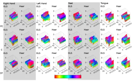
Figure 4.Average detail coefficients corresponding to the third level of decomposition for the subject C-3 using both GLS and Haar wavelets. The original segment was taken att= 4s
and had a length of 256 samples.The data is split by classes so the different arising pattenrs are visible. The y axis represents the sample number and the x axis the electrode.
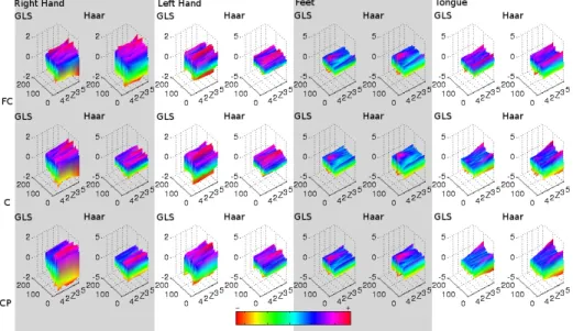
Figure 5.Average approximation coefficients corresponding to the first level of decomposition for the subject C-3 using both GLS and Haar wavelets. The original segment was taken at
t= 4sand had a length of 256 samples. The data is split by classes so the different arising pattenrs are visible. The y axis represents the sample number and the x axis the electrode.
Figure 6. Average approximation coefficients corresponding to the third level of decomposition for the subject C-3 using both GLS and Haar wavelets. The original segment was taken att = 4sand had a length of 256 samples. The data is split by classes so the different arising pattenrs are visible. The y axis represents the sample number and the x axis the electrode.
the energy in different temporal-spatial locations. On the other hand, Figure 5 and Figure 6 show a similar behaviour on the approximation coefficients on the first level for both wavelets, although the effect of the graph scheme becomes apparent on the third level.
Another interesting property showed by the GLS is the amount of energy produced by the detail coefficients. In Table 1, we observe that the new approach produces, in general, details with less energy than Db5 or, in other words, the error of approximating the original signals using GLS is smaller. This is true for the last four levels, although the energy in levels one and two is significantly higher for the graph based approach. The reason for this behaviour is the fact that the signal has been previously filtered between 8 and 30 Hz, and therefore we should expect Db5 to produce near to zero coefficients in the highest frequency bands. For Db5 the frequency bands for each level are: level 1,128−256Hz; level 2,64−128Hz; level 3,32−64Hz; level 4,16−32Hz; level 5,8−4Hzand level 6,4−2Hz. On the other hand, we can no longer refer to frequency bands in the graph lifting as the detail coefficients are enriched with the spatial information of the surrounding nodes. The behaviour of both decompositions is coherent with the correlation between amplitude and frequency present in EEG data. The energy of the signals decrease as we lower the frequency of analysis, obtaining relative small values at the end of the decomposition tree.
Another benefit from the lifting scheme is a low computational requirement. The whole trial decomposition is reduced to two matrix multiplications, decreasing by 20 times the processing time required when compared with a standard DWT implementation during the experiments.
Table 2 for the Essex dataset and Table 3 for the competition dataset show the Kappa values and the mean accuracy achieved using the experimental methodology explained in Section 2.6. Analysing the results, we can infer that the simple graph based approach performed better than any other approach on 85% of the subjects. A Wilcoxon’s ranksum test
Table 1.Comparison of the averaged energy between Graph and Db5 in the detail coefficients
Level Eng EnDb5 Hypothesis p-value
1 0.674±1.360 0.000±0.000 Eng≥EnDb5 p <0.05 2 0.105±0.250 0.039±0.046 Eng≥EnDb5 p <0.05 3 0.139±0.147 0.475±0.387 Eng≤EnDb5 p <0.05 4 0.085±0.080 1.424±1.679 Eng≤EnDb5 p <0.05 5 0.019±0.025 0.228±0.297 Eng≤EnDb5 p <0.05 6 0.006±0.011 0.034±0.043 Eng≤EnDb5 p <0.05 Mean 0.171±0.613 0.366±0.872 Eng≤EnDb5 p <0.05
Table 2.Results on the Essex dataset in terms of Kappa values. The mean accuracy is included at the bottom.
Subject Haar Db5 Linear LS GLS
E-1 0.399 0.389 0.469 0.504 E-2 0.526 0.336 0.475 0.584 E-3 0.401 0.449 0.375 0.421 E-4 0.421 0.361 0.453 0.790 E-5 0.267 0.239 0.224 0.268 E-6 0.296 0.215 0.313 0.354 E-7 0.419 0.401 0.509 0.683 E-8 0.096 0.037 0.057 0.130 E-9 0.296 0.200 0.275 0.356 E-10 0.362 0.446 0.446 0.622 E-11 0.194 0.144 0.110 0.121 E-12 0.244 0.261 0.202 0.346 Mean Kappa 0.327 0.290 0.326 0.432 ± ± ± ± 0.11 0.12 0.15 0.21 Mean Acc 0.553 0.527 0.551 0.624 ± ± ± ± 0.07 0.08 0.10 0.13
proves that this difference is statistically significant (p < 0.05) when comparing the graph approach with FWGs or the linear lifting scheme. This outcome gives evidence that FGW may not be the best MRA approach when dealing with MI-EEG data for BCI.
The reason for this improvement can be seen in Figure 7, which shows the averaged Kappa values over all the subjects in each level and each segment as a density plot. Each density plot is accompanied by the mean Kappa values for each level and each temporal segment. It is interesting to see how the GLS increases the Kappa values as effect of introducing the spatial information in those frequency bands filtered during the preprocessing. Examining the mean Kappa values per level and per segment we see that the performance for the graph decomposition is higher for all the segments and levels (apart from the level 6) when compared to Db5.
In Figure 8 we see how the tendency observed in Figure 7 regarding the Kappa value distribution per level is consistent for high scoring subjects, while low scoring subjects tend to develop a more sparse Kappa value distribution along the multiresolution analysis.
Table 3.Results on the competition dataset in terms of Kappa values. The mean accuracy is included at the bottom.
Subject Haar Db5 Linear LS GLS
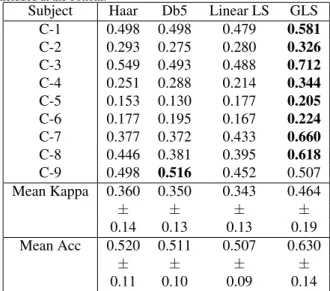
C-1 0.498 0.498 0.479 0.581 C-2 0.293 0.275 0.280 0.326 C-3 0.549 0.493 0.488 0.712 C-4 0.251 0.288 0.214 0.344 C-5 0.153 0.130 0.177 0.205 C-6 0.177 0.195 0.167 0.224 C-7 0.377 0.372 0.433 0.660 C-8 0.446 0.381 0.395 0.618 C-9 0.498 0.516 0.452 0.507 Mean Kappa 0.360 0.350 0.343 0.464 ± ± ± ± 0.14 0.13 0.13 0.19 Mean Acc 0.520 0.511 0.507 0.630 ± ± ± ± 0.11 0.10 0.09 0.14
Figure 7. Density plots of the Kappa values achieved on the evaluation data averaged over all the subjects. a)andb)correspond to the Kappa values achieved by the detail and approximation coefficient sets for GLS respectively,c)andd)correspond to Db5. The Y-axis represents each level of decomposition meanwhile the X-Y-axis represents the temporal segments. The boxplots over the density values correspond to the mean Kappa values over the segments (on top) and the accumulated Kappa values over the levels (on the right).
Figure 8. Density plots of the Kappa values achieved by the detail coefficients of GLS per segment and level of decomposition for two different subjects.a)Corresponds to subject E-7, andb)to subject E-8. High scoring subjects such as E-7 tend to have more compact Kappa value density plots.
Figure 9. Density plots of the Kappa values achieved by the detail and approximation coefficients by GLS per segment and level of decomposition for subject E-1 on the training set. This information can be used to select a basis for the evaluation set.
The obtained results can be easily enhanced by making use of the Kappa density plots. A simple heuristic can be proposed as best basis selection algorithm by simply selecting those levels and segments which perform the best on the training set. Figure 9 shows the distribution of the Kappa value for the subject E-1 when classifying the training set. In this case we can select the 5th level from the detail coefficients and from the 2nd to the 5th level from the approximation coefficients as they provide high Kappa values. The first five segments will be discarded as their colour in the density plot indicate a poor Kappa value. With the newly selected basis, the performance of classifying the evaluation set is increased from0.50to
0.63. However this procedure is highly time consuming, and therefore, it could be performed by automatic best basis selection methods such as local discriminant bases [27].
The performance achieved by the initially designed GLS would score the third place among the BCI competition results, although it is far from the0.57of Kappa value obtained by the competition winner. The feature extraction method exposed in Section 2.4 may be too naive to achieve a high classification accuracy. Therefore, in order to increase the performance, we propose to enhance the feature extraction using common spatial patterns (CSP), as it is broadly used in the literature and it has been proved to lead to high classification
Table 4.Results on the competition data set expressed as Kappa value for the proposed method using CSP and the winner from the BCI competition IV
Subject GLS + CSP Competition winner
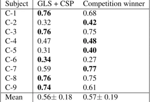
C-1 0.76 0.68 C-2 0.32 0.42 C-3 0.76 0.75 C-4 0.47 0.48 C-5 0.31 0.40 C-6 0.34 0.27 C-7 0.59 0.77 C-8 0.76 0.75 C-9 0.74 0.61 Mean 0.56±0.18 0.57±0.19
performance. As proposed in other studies, CSP was applied over each coefficient set [28] [29], projecting the signals onto the space defined by the transformation matrix, and calculating the logarithm of the sum of the three first and three last components [30].
The obtained results from applying CSP at each level and each segment are comparable to those achieved by the competition winner as shown in Table 4, even though our classification model is simpler than the one used in the competition, in which an one-against-the-rest naive bayes classifier was used and the CSP features were selected using mutual information [31]. A baseline Kappa value for comparison is given by applying CSP on the first level (original signal only) which results in an average Kappa value of0.52±0.21.
4. Conclusions
This study is a first attempt of applying MRA over graphs to extract temporal-spatial-spectral features for BCI applications. Overall, we have built a new LS that obtains better classification performance for 85% of the subjects studied than FGWs under the same conditions. Even with simple feature extraction techniques, the proposed method is able to achieve competitive results.
It is indicated that the classification performance can be improved by choosing a more sophisticated experimental setup. In the present study we show how using a more complex feature extraction method, namely CSP, leads to results comparable to ones achieved by the competition winner. Selecting an appropriate basis is also a common approach when dealing with MRA data, and we have presented proofs on how this fact also applies to GLS, leaving room for more improvement in the future research.
The proposed method has proved to obtain valuable information from the decomposition coefficients where first generation wavelets are incapable due to their design principles. The addition of spatial information to the MRA decomposition contributes to a more complete signal representation, but we have not yet explored the benefits of this approach in a packet based model.
The possibilities to follow this line of research for further investigation are enormous. The static graph structure proposed here can be rearranged in various manners to better extract classification features, like adding connections with various time delays to improve the shift-invariant properties of the analysis. Dynamic graph generation to exploit user specific data relationships could be another improvement to the basic model.
The update and predict functions proposed here can also be easily modified and improved. A weighted Laplacian filter definition would allow fine tuning of the decomposition and obtain more interesting features. Other approaches such as B-spline interpolation could also result in highly interesting performance. We can also think of approaches that adapt the functions aiming at the class separability instead of focusing on energy minimisation. Acknowledgments
The first author would like to thank the EPSRC for funding his Ph.D. study via an EPSRC DTA award.
References
[1] A. Nijholt and D. Tan. Brain-computer interfacing for intelligent systems.IEEE Intelligent Systems, 23(3):72– 79, 2008.
[2] J. J. Vidal. Toward direct brain-computer communication. Annual Review of Biophysics and Bioengineering, 2(1):157–180, 1973.
[3] G. Pfurtscheller and F. H. Lopes da Silva. Event-related EEG/MEG synchronization and desynchronization: basic principles. Clinical Neurophysiology, 110(11):1842–1857, 1999.
[4] I. Daubechies. Ten Lectures on Wavelets. Society for Industrial and Applied Mathematics, 2006.
[5] W. Sweldens. The lifting scheme: A construction of second generation wavelets. SIAM Journal on Mathematical Analysis, 29(2):511, 1998.
[6] M. Murugappan, M. Rizon, R. Nagarajan, S. Yaacob, I. Zunaidi, and D. Hazry. Lifting scheme for human emotion recognition using EEG. InInternational Symposium on Information Technology., volume 2, pages 1–7. IEEE, 2008.
[7] B. Graimann, J. E. Huggins, S. P. Levine, and G. Pfurtscheller. Toward a direct brain interface based on human subdural recordings and wavelet-packet analysis. IEEE Transactions on Biomedical Engineering, 51(6):954–962, 2004.
[8] S. K Narang and A. Ortega. Lifting based wavelet transforms on graphs. InConference of Asia-Pacific Signal and Information Processing Association, pages 441–444, 2009.
[9] C. Brunner, R. Leeb, G. R. Muller-Putz, A. Schlogl, and G. Pfurtscheller. BCI competition 2008 - Graz data set A. http://www.bbci.de/competition/iv/desc_2a.pdf, 2008.
[10] M. Naeem, C. Brunner, R. Leeb, B. Graimann, and G. Pfurtscheller. Seperability of four-class motor imagery data using independent components analysis. Journal of neural engineering, 3(3):208, 2006.
[11] C. Brunner, R. Leeb, G. R. Muller-Putz, A. Schlogl, and G. Pfurtscheller. BCI competition 2008 Graz data set A. 2009.
[12] E. Aboufadel and S. Schlicker. Discovering Wavelets. Wiley Online Library, 1999. [13] P. S Addison. The Illustrated Wavelet Transform Handbook. Institute of Physics Publ., 2002.
[14] V. Bostanov. BCI competition 2003-data sets Ib and IIb: feature extraction from event-related brain potentials with the continuous wavelet transform and the t-value scalogram. IEEE Transactions on Biomedical Engineering, 51(6):1057–1061, 2004.
[15] B. G. Xu and A. G. Song. Pattern recognition of motor imagery EEG using wavelet transform. J. Biomedical Science and Engineering, 1:64–67, 2008.
[16] J. Sherwood and R. Derakhshani. On classifiability of wavelet features for EEG-based brain-computer interfaces. InInternational Joint Conference on Neural Networks., pages 2895–2902. IEEE, 2009. [17] S. Yan, H. Zhao, C. Liu, and H. Wang. Brain-computer interface design based on wavelet packet transform and
SVM. InInternational Conference on Systems and Informatics, pages 1054–1056. IEEE, 2012.
[18] B. Yang, G. Yan, R. Yan, and T. Wu. Adaptive subject-based feature extraction in braincomputer interfaces using wavelet packet best basis decomposition. Medical Engineering & Physics, 29(1):48–53, 2007. [19] B. Yang, G. Yan, T. Wu, and R. Yan. Subject-based feature extraction using fuzzy wavelet packet in
braincomputer interfaces. Signal Processing, 87(7):1569–1574, 2007.
[20] W. Ting, Y. Guo-zheng, Y. Bang-hua, and S. Hong. EEG feature extraction based on wavelet packet decomposition for brain computer interface. Measurement, 41(6):618–625, 2008.
[21] W. Sweldens. Wavelets and the lifting scheme: A 5 minute tour. Zeitschrift fur Angewandte Mathematik und Mechanik, 76(2):41–44, 1996.
[22] R. L Claypoole Jr, R. G Baraniuk, and R. D Nowak. Adaptive wavelet transforms via lifting. InIEEE International Conference on Acoustics, Speech and Signal Processing., volume 3, pages 1513–1516. IEEE, 1998.
[23] E. Martinez-Enriquez and A. Ortega. Lifting transforms on graphs for video coding. InData Compression Conference, pages 73–82. IEEE, 2011.
[24] M. Wardetzky, S. Mathur, F. Kalberer, and E. Grinspun. Discrete Laplace operators: no free lunch. InACM International Conference Proceeding Series, volume 257, pages 33–37, 2007.
[25] B. Blankertz, K. R Muller, D. J Krusienski, G. Schalk, J. R Wolpaw, A. Schlogl, G. Pfurtscheller, J. R Millan, M. Schroder, and N. Birbaumer. The BCI competition III: validating alternative approaches to actual BCI problems. IEEE Transactions on Neural Systems and Rehabilitation Engineering, 14(2):153–159, 2006. [26] J. Cohen. A coefficient of agreement for nominal scales. Educational and Psychological Measurement,
20(1):37–46, 1960.
[27] N. F Ince, A. H Tewfik, and S. Arica. Extraction subject-specific motor imagery time-frequency patterns for single trial EEG classification. Computers in Biology and Medicine, 37(4):499–508, 2007.
[28] E. A Mousavi, J. J Maller, P. B Fitzgerald, and B. J Lithgow. Wavelet common spatial pattern in asynchronous offline brain computer interfaces. Biomedical Signal Processing and Control, 6(2):121–128, 2010. [29] J. Asensio-Cubero, J. Q. Gan, and R. Palaniappan. Extracting common spatial patterns based on wavelet lifting
for brain computer interface design. InThe 4th Computer Science and Electronic Engineering Conference (CEEC), pages 160–163. IEEE, 2012.
[30] H. Ramoser, J. Muller-Gerking, and G. Pfurtscheller. Optimal spatial filtering of single trial eeg during imagined hand movement. IEEE Transactions on Rehabilitation Engineering, 8(4):441–446, 2000. [31] C. Zheng Yang, W. Chuanchu, G. Cuntai, Z. Haihong, P. Kok Soon, H. Brahim, and T. Keng Peng. BCI
competition IV dataset 2a submission by institute for infocomm research, agency for science, technology and research singapore I2R, A*STAR. http://www.bbci.de/competition/iv/results/ds2a/ KaiKengAng_desc.pdf, 2008.