Air Force Institute of Technology
AFIT Scholar
Theses and Dissertations Student Graduate Works
3-24-2016
An Evaluation of Forecasting Methods that Could
be Used in the Brazilian Air Force Uniform
Distribution Process
Leandro Valviesse de OliveiraFollow this and additional works at:https://scholar.afit.edu/etd
Part of theOperations and Supply Chain Management Commons
This Thesis is brought to you for free and open access by the Student Graduate Works at AFIT Scholar. It has been accepted for inclusion in Theses and Dissertations by an authorized administrator of AFIT Scholar. For more information, please [email protected].
Recommended Citation
Oliveira, Leandro Valviesse de, "An Evaluation of Forecasting Methods that Could be Used in the Brazilian Air Force Uniform
Distribution Process" (2016).Theses and Dissertations. 374.
AN EVALUATION OF FORECASTING METHODS THAT COULD BE USED IN THE BRAZILIAN AIR FORCE UNIFORM DISTRIBUTION PROCESS
THESIS MARCH 2016
Leandro Valviesse de Oliveira, Captain, Brazilian Air Force AFIT-ENS-MS-16-M-122
DEPARTMENT OF THE AIR FORCE AIR UNIVERSITY
AIR FORCE INSTITUTE OF TECHNOLOGY
Wright-Patterson Air Force Base, OhioDISTRIBUTION STATEMENT A.
The views expressed in this thesis are those of the author and do not reflect the official policy or position of the United States Air Force, Department of Defense, or the United States Government, the corresponding agencies of any other government, the North Atlantic Treaty Organization or any other defense organization.
AFIT-ENS-MS-16-M-122
AN EVALUATION OF FORECASTING METHODS THAT COULD BE USED IN THE BRAZILIAN AIR FORCE UNIFORM DISTRIBUTION PROCESS
THESIS
Presented to the Faculty Department of Operational Sciences Graduate School of Engineering and Management
Air Force Institute of Technology Air University
Air Education and Training Command In Partial Fulfillment of the Requirements for the
Degree of Master of Science in Logistics and Supply Chain Management
Leandro Valviesse de Oliveira Captain, Brazilian Air Force
March 2016
DISTRIBUTION STATEMENT A.
AFIT-ENS-MS-16-M-122
AN EVALUATION OF FORECASTING METHODS THAT COULD BE USED IN THE BRAZILIAN AIR FORCE UNIFORM DISTRIBUTION PROCESS
Leandro Valviesse de Oliveira Captain, Brazilian Air Force
Committee Membership:
Dr. Jeffrey Ogden Chair
Dr. Michael Kretser Member
iv AFIT-ENS-MS-16-M-122
Abstract
Every year the Brazilian Air Force (BAF) spends the equivalent of approximately 15 million dollars for uniforms. These purchases come from a tight budget, are executed through public procurement processes, and are tied to Brazilian acquisition regulations, which are often very strict. For this reason, lead times are unpredictable. It can take anywhere from one month to a year to replenish an item.
The purpose of this research is to analyze the forecasting process performed at a BAF military organization named Sub-directorate of Supply (SDS) with the intent of building an algorithm comprised of a selection of forecasting models in order to help SDS optimize its inventory investments.
With this in mind, monthly sales, prices, and inventory records from January of 2010 to July of 2015 were extracted from a database and converted to a standard spreadsheet format. Several forecasting models were evaluated and applied to randomly selected items from the database to create the algorithm.
In the final analysis, it was concluded that two models precisely depicted the behavior of sales in BAF’s stores. These two models were then utilized to develop the forecasting tool that may prove valuable in future BAF uniform purchasing decisions.
v AFIT-ENS-MS-16-M-122
My eternal love and gratitude to my wife, for your priceless love, support, understanding, and words of encouragement that have always made me reach farther.
vi
Acknowledgments
I wish to thank my committee members who were more than generous with their
expertise and precious time. A special thanks to Dr. Jeffrey Ogden, for his guidance and support throughout the course of this thesis effort. The insight and experience was certainly appreciated. I would also like to thank my reader, Dr. Michael Kretser for his valuable contribution to this research endeavor. His comments and expertise were highly appreciated.
I am forever indebted to Mrs. Annette Robb, International Military Student Officer, to Mrs. Clara Delgado for their encouraging contributions in new language adaptation; and Mr. Victor Grazier for reviewing my work. Their participation was essential to the success of this study.
Finally, I would like to thank my classmates, American and International Students, who were very supportive throughout this program. I truly valued your contributions, team efforts, and friendship.
vii
Table of Contents
Abstract ... iv
Table of Contents ... vii
List of Figures ... x List of Tables ... xi I. Introduction ... 1 Purpose ... 1 Background ... 1 Problem Statement ... 3 Research Objectives ... 3 Research Questions ... 4 Methodology ... 4
Assumptions and Limitations of the Study ... 5
Organization ... 5
II. Literature Review ... 7
Overview ... 7
Methods ... 7
Forecasting and Inventory Control ... 9
Statistical Significance Assessment ... 11
Forecast Quality ... 12
Smoothing the Bullwhip Effect in Seasonal Supply Chains ... 15
Forecasting Role in the Supply Chain (Costantino, Di Gravio, Shaban, & Tronci, 2015) ... 16
What Experts Say ... 17
Simple Versus Complex Forecasting ... 18
Forecastability ... 20
Combining Forecasts ... 21
Forecasting and Inventory Control ... 23
III. Methodology ... 25
Overview ... 25
Data Collection ... 25
Item Selection ... 27
viii
Methodology Used to Address the Research Questions ... 28
1. What metrics are currently being utilized by the Supply Division? ... 28
2. How can the forecasting process for uniform sales be improved in the SDS? ... 28
3. How to best assess accuracy of forecasting sales in the SDS? ... 37
4. Is it possible to build an algorithm where historical sales data can be evaluated and the best forecast suggested? ... 42
IV. Results and Analysis ... 44
Overview ... 44
Forecasting in place at SDS ... 44
Forecasting methods ... 47
Practical use of the algorithm ... 53
Coat ... 54 Trousers ... 56 T-shirt ... 58 Hat ... 60 Final dispositions ... 62 V. Discussion ... 65 Overview ... 65
The Process Currently in Place ... 65
Similar Studies ... 67
Conclusion ... 68
Recommendations ... 71
Limitations ... 73
Future Research ... 73
Appendix A. Naïve forecast sample ... 75
Appendix B. Simple Linear Regression sample ... 76
Appendix C. Trend... 77
Appendix D. Dummy variables ... 78
Appendix E. Trigonometry (4-year cycle) ... 79
Appendix F. Trigonometry (2-year cycle) ... 80
Appendix G. Trigonometry (1-year cycle) ... 81
Appendix H. Autocorrelation (4-year cycle) ... 82
ix
Appendix J. Autocorrelation (1-year cycle)... 84
Appendix K. Decomposition Multiplicative (12 months) ... 85
Appendix L. Decomposition Multiplicative (4 months) ... 86
Appendix M. Decomposition Additive (12 months) ... 87
Appendix N. Simple Exponential Smoothing ... 88
Appendix O. Holt's Trend Corrected ... 89
Appendix P. Additive Holt-Winters (4 months) ... 90
Appendix Q. Additive Holt-Winters (12 months) ... 91
Appendix R. Multiplicative Holt-Winters (4 months) ... 92
Appendix S. Multiplicative Holt-Winters (12 months) ... 93
Appendix T. ARIMA ... 94
Appendix U. Comparison Chart item 1 - St Dumont medal 20yrs ... 95
Appendix V. Comparison Chart item 2 - PT short officer women ... 96
Appendix W. Comparison Chart item 3 - Blue skirt ... 97
Appendix X. Comparison Chart item 4 – Collar insignia ... 98
Appendix Y. Comparison Chart item 5 – Plastic clip ... 99
Appendix Z. Comparison Chart item 6 – White Air Force t-shirt ... 100
Appendix AA. Comparison Chart item 7 – Shoulder badge ... 101
Appendix AB. Comparison Chart item 8 – 2nd Sgt hat badge ... 102
Appendix AC. Comparison Chart item 9 – Blue jacket for men ... 103
Appendix AD. Comparison Chart item 10 – ABU Blouse ... 104
Appendix AE. Comparison Chart item 11 – Blue hat for men ... 105
Appendix AF. Comparison Chart - Algorithm – ABU Coat ... 106
Appendix AG. Comparison Chart - Algorithm – ABU Hat ... 107
Appendix AH. Comparison Chart - Algorithm – ABU Trousers ... 108
Appendix AI. Comparison Chart - Algorithm – ABU T-shirt ... 109
Appendix AJ. Comparison Chart - Algorithm – Black buckle ... 110
Appendix AK. Comparison Chart - Algorithm – Black sock ... 111
Appendix AL. Thesis quad chart ... 112
x
List of Figures
Figure 1. Automated vertical storage in SDS ... 45
Figure 2. Example of the comparison between Sales and Inventory ... 47
Figure 3. Validity assumptions for coat forecasting residuals ... 55
Figure 4. Graphical output of forecasted values ... 56
Figure 5. Validity assumptions for trousers forecasting residuals ... 57
Figure 6. Graphical output of forecasted values ... 58
Figure 7. Validity assumptions for t-shirt forecasting residuals ... 59
Figure 8. Graphical output of forecasted values ... 60
Figure 9. Validity assumptions for hat forecasting residuals ... 62
xi
List of Tables
Table 1. ARIMA identification ... 35
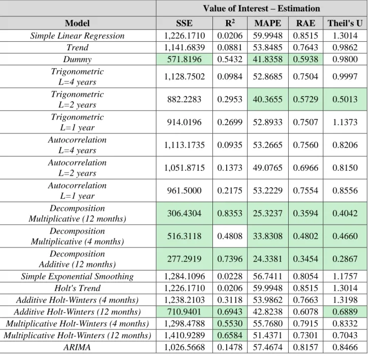
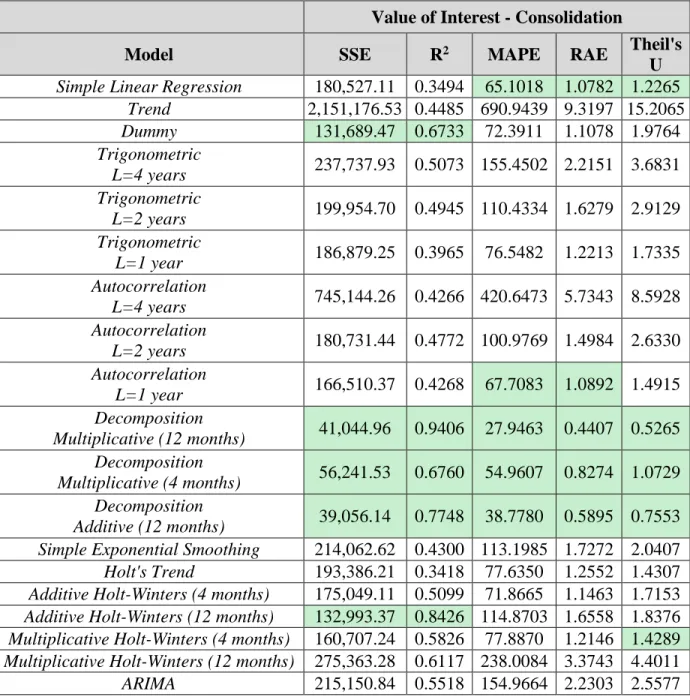
Table 2. Example of a comparison chart for the estimation period ... 48
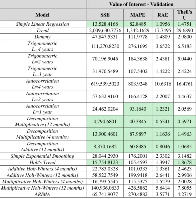
Table 3. Example of a comparison chart for the validation period ... 49
Table 4. Example of a consolidation chart ... 50
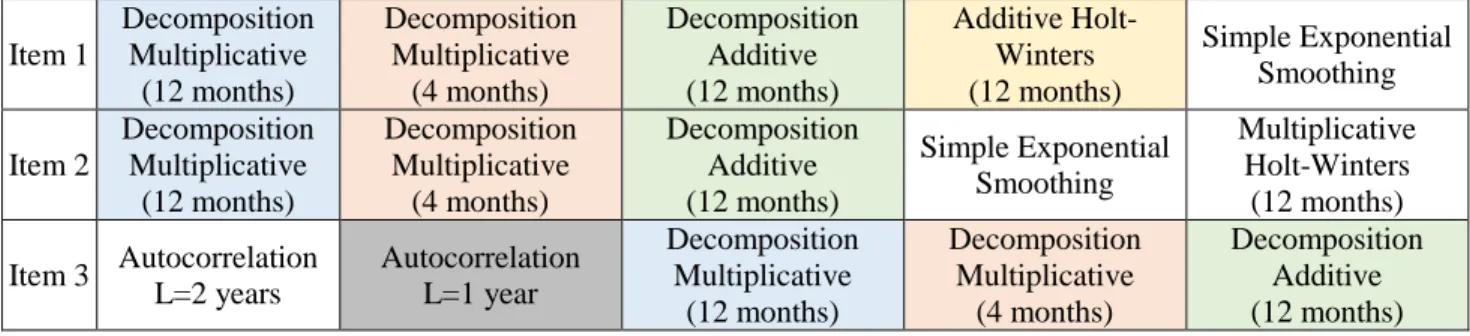
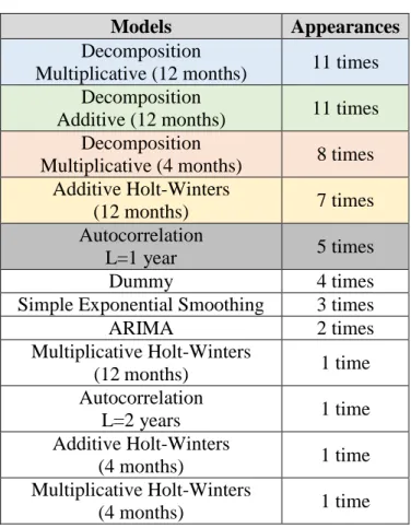
Table 5. Models selection ... 51
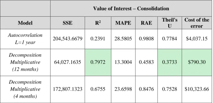
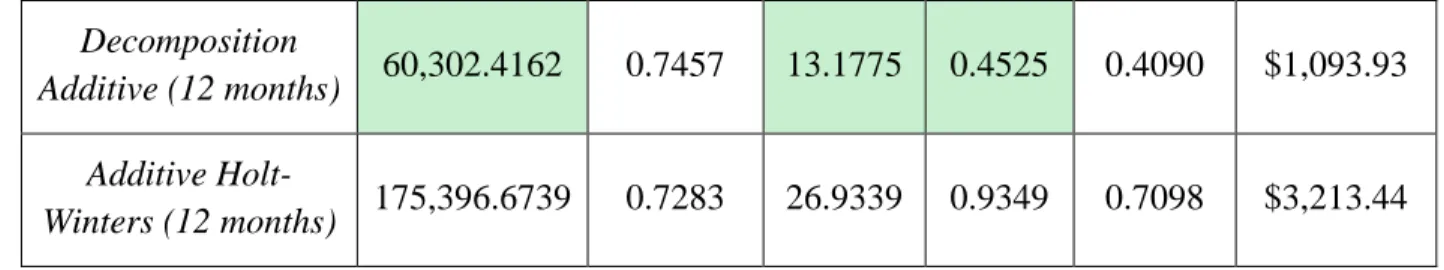
Table 6. Final models’ accountability ... 53
Table 7. Algorithm output for coat sales forecast ... 54
Table 8. Algorithm output for trousers sales forecast ... 56
Table 9. Algorithm output for t-shirt sales forecast ... 58
Table 10. Algorithm output for hat sales forecast ... 60
Table 11. Algorithm output for black buckle sales forecast ... 63
1
AN EVALUATION OF FORECASTING METHODS THAT COULD BE USED IN THE BRAZILIAN AIR FORCE UNIFORM DISTRIBUTION PROCESS
I. Introduction Purpose
Every year the Brazilian Air Force (BAF) spends the equivalent of approximately 15 million dollars in uniforms for its military. These purchases come from a tight budget and are executed through public procurement processes, according to the Brazilian acquisition
regulations. This compendium of regulations obliges the bidding commission to always buy from the cheapest supplier. Despite having issues in this area, this research will focus on the previous step to acquisition itself: the forecast.
The purpose of this research is to analyze a process performed by the Supply Division of a BAF military organization named Sub-directorate of Supply (SDS). This study aims to
identify opportunities for improvement as well as applicable performance evaluation metrics that could be applied to the process in order to drive management actions toward quality and
performance enhancements. The actual expected product of this study, however, is an algorithm comprising a selection of forecasting models that can be valuable in purchasing decisions in the future.
Background
The Sub-directorate of Supply, located in São Paulo, is the main unit in theBAF responsible for forecasting, acquiring, and distributing uniforms. The process of uniform
2
distribution is performed through two main depots. The first is stationed inside the boundaries of SDS. The second is located in Rio de Janeiro, in a Unit named Intendancy Central Depot (ICD). From these two units, uniform items are distributed to warehouses located in 64 Air Force Bases, which will distribute either to end-users (i.e. militaries), or to other lower-level units.
The ranks in BAF are distributed as enlisted and officers. The enlisted ranks are, literally translated, Recruits, First-class Soldiers, Corporals, Third Sergeant, Second Sergeant, First Sergeant, and Sub-officer. The officer ranks are Second Lieutenant, First Lieutenant, Captain, Major, Lieutenant Colonel, and Colonel. All Recruits, First-class Soldiers, andCorporals are entitled to use their uniforms while serving the Air Force, receiving them from the respective organizations they are assigned to, free of charge. At pre-determined periods of time (which varies according to the uniform) they have the right to renew their uniforms. Either when renewing or leaving the active duty, they are expected to return every piece of uniform found in their possession.
In contrast, all military members with ranks of Third Sergeant and above are eligible to receive a military clothing allowance. These military personnel can buy their uniforms in one of the 29 Regional Uniform Stores (RUS) dispersed around the country, positioned inside BAF Units.
This research focuses on the latter case as it aims to setup a framework that can be applied to a specific sales behavior. However, the results can certainly be beneficial for both cases, serving as a starting point to a variety of cases such as previously described, related to whom is entitled to the right of receiving their uniforms free of charge.
3
Problem Statement
Initially, it was detected that the volume of sales and inventory levels were incompatible, with excess inventory for some items, and empty shelves for others. Furthermore, after
analyzing the process for forecasting uniform sales, there was a visible sign that no scientific methods are currently being used to predict how much of each item has to be purchased to replenish the warehouse.
Additionally, there does not appear to be a procedure or metric currently in place at the Supply Division regarding its inventory policy. Ultimately, the unpredictable lead time for most of the items, due to Brazil`s acquisition regulations, further complicates the decisionfor
managers to determine what inventory policy to use.
Research Objectives
The primary objective of this research was to identify potential flaws in the forecasting process that could be recognized as ineffective and inefficient, proposing potential solutions according to the literature on this subject. This would allow proposing specific actions for enhancing the overall performance of the Supply Division in SDS.
Secondarily, this research attempted to recommend an algorithm with a set or a
combination of forecasting models that enhances the SDS acquisitions, enabling all the 29 RUSs to have the right items, at the right moment, in the right amount. The concept was that the algorithm had to be functional and easily implementable.
4
Research Questions
In order to address the objectives outlined for this study, some investigative questions were formulated and needed to be answered throughout the paper, as follows:
1. What metrics are currently being utilized by theSupply Division?
2. How can theforecasting process for uniform sales be improved in theSDS?
3. How to best assess accuracy of forecasting sales in theSDS?
4. Is it possible to build an algorithm where historical sales data can be evaluated and the best forecast suggested?
Methodology
The present study is mainly quantitative, although some qualitative aspects related to the context in which forecasting is being processed in SDS had to be clarified in order to provide the necessary support for the research. With this intention, SDS regulations were examined in order to identify what categories of metrics were effective in the timeframe researched. Moreover, information regarding this feature was obtained from the responses provided in an interview with the head of the Supply Division.
As far as the quantitative part, all aspects of the data collection and cleansing, as well as the tools employed, were given special care in order to preserve reliability in the results.
A deep analysis throughout a variety of forecast methods and accuracy parameters was performed with care prior to their selection. In addition, all formulas were written from scratch to ensure exactness of the calculations. Afterwards, a comparison chart was built to facilitate
5
displaying and highlighting the best results. Further details on the methodology used in this research are stated in Chapter III.
Assumptions and Limitations of the Study
An important assumption in this study was that an accurate forecasting process results in valuable data that serves as a subsidy to allow management to make reasonable decisions on purchasing, given the current inventory policies.
The focus of this study was primarily quantitative, although it is evident that the subject covered in this paper is directly attached to qualitative aspects. In other words, forecasting is strictly related to inventory control and lead times. The latter two, despite being sensitive issues in SDS, were not treated by the present research. Thus, this research focused strictly on the calculations involving the forecasting process, not with their interaction.
The absence of metrics currently being taken regarding inventory holding cost rate on inventory policies, such as storage, obsolescence, and opportunity costs (as well as accurate information about lead times) prevented a more comprehensive approach to the problems revealed.
Organization
Chapter I offers the necessary background to understand the context of the process under study as well as provides the purpose, the problem that was brought to attention, the objectives of this research and the research questions. Chapter I also provides an overview on the theoretical
6
background that guided the analysis and on the methodology along with some of the assumptions and limitations applied to this study.
Chapter II gives a conceptual foundation with the theoretical background that guided this research in terms of the methodology adopted for data analysisand accuracy measurements, expressing the opinions of experts concerning the concepts covered.
Chapter III gives special attention to applying the methodologies used in this research, particularly with respect to the procedure for data collection, statistical analysis, and the criteria adopted.
Chapter IV analyzes and displays the results obtained by applying the models developed in this study in an attempt to solve the problem and answer the Research Questions previously stated. Also in this chapter, further investigation exposed thoughts necessary to exhaust the possibilities and produce solid outcomes.
Chapter V presents the conclusions of this research, as well as recommendations for further investigation in the area.
7
II. Literature Review
Overview
This chapter explores theoretical perspectives and previous research findings that can help in developing a tailored response for the analysis to be performed in the present research. It contains aspects, such as some key methods available, the relationship between forecasting and inventory control, assessment of statistical significance, forecasting accuracy, comparison
between simple and complex forecasting, and procedures and rules used for combining forecasts.
Methods
In the book “Principles of Forecasting,” Professor John Scott Armstrong of the Wharton
School, University of Pennsylvania, addresses problems related to finance, marketing, personnel, and production, covering all types of forecasting methods: judgmental methods, such as Delphi, role-playing, and intentions studies, and quantitative methods, including econometric methods, expert systems, and extrapolation. Some methods, such as conjoint analysis, analogies, and rule-based forecasting, integrate quantitative and judgmental procedures. In each area, he identifies what is known as “if-then clauses” (e.g. “if the results are required tomorrow, then I will need two additional people to perform testing today”) and summarizes evidence on these principles (JS Armstrong, 2002).
Nevertheless, before reaching a higher level of knowledge, it is important to start with basic principles, rules, and definitions. Following, they are briefly presented in order to provide the reader with an initial framework.
8
There are two broad categories of forecasting techniques: qualitative methods and quantitative methods. According to Hyndman & Athanasopoulos, (2014), qualitative methods are well-developed, structured approaches to obtaining good forecasts without using historical data, while quantitative methods are based on algorithms of varying complexity and can be applied when two conditions are satisfied. These conditions are: numerical information about the past is available, and it is reasonable to assume that some aspects of the past patterns will continue into the future (Hyndman & Athanasopoulos, 2014).
There is a wide range of quantitative forecasting methods, often developed within specific disciplines for specific purposes. Each method has its own properties, accuracies, and costs that must be considered when choosing a specific method. Most quantitative forecasting problems use either time series data (collected at regular intervals over time) or cross-sectional data (collected at a single point in time) (Bowerman, Connell, & Koehler, 2005).
Time series data are of interest for this study as the data collected refers to sales
information encompassing 67 months. This type of data is particularly useful when one wants to forecast something that is happening over time and thus is subject to externalities. These
methods can be the simplest to deploy and yet quite accurate, particularly over the short term. Quantitative forecasting methods analyze patterns in historical data in an attempt to use past patterns to predict future patterns.
The methods designed for time series can use models as simple as the moving average or as complex as the ARIMA models. In the first case, the forecast is the average of the previous determined number “x” of observations or periods, where "x" is a number that best apply for that time series. For instance, if there is monthly sales data being forecasted, a 12-month (period)
9
moving average might be used, where always the forecast for the next month is the average over the past 12 months.
Simple averaging observations, however, may not work well enough when there is trend or seasonality in the data. In that case, other techniques, such as exponential smoothing, may be more appropriate.
With moving average, every data point has identical weight in calculating forecast. With smoothing methods, more importance is placed on the most recent data than on the historical data. If there is trend present in the data, placing more weight in recent observations will make the forecast more likely to reproduce the trend.
Moving averages and simple exponential smoothing techniques are available in Excel and easy to execute. That is part of the great advantage of time series methods: they are generally simple, cheap to run, and relatively easy to interpret (Hyndman & Athanasopoulos, 2014).
There are more complex time series techniques as well, such as Box-Jenkins models that can deal with data with trends and seasonality. The Box-Jenkins ARIMA model is a
combination of the AR (autoregressive) and MA (moving average) models, with the "I" standing for "Integrated" (NIST/SEMATECH, 2013). Chapter III will provide more in-depth descriptions of the methods and their models selected to perform the data analysis in this study.
Forecasting and Inventory Control
According to Gardner (1990), “forecasting is a prerequisite to inventory decisions in practice”. This topic appears very convenient to be discussed since it has the scope of combining forecasting and inventory control. In fact, the decision over inventory strategy can be made over
10
a tradeoff curve between service level and inventory investment. By improving forecast accuracy this curve should be shifted in such a way that both improves customer service and reduces inventory investment. To accomplish such calculations, a high number of metrics should be taken into account, most of which do not exist in the Military Organization focus of this study.
Although a combination of Forecasting and Inventory Control would be the perfect approach for this study, as will be seen in Chapter IV, the inventory policies in Sub-directorate of Supply (SDS) are complex enough for another thesis topic, due to several aspects. Here we can emphasize, as an example, the unpredictable lead times that result from the Brazilian Acquisition Law. As Arraes, K. G. G. observed, “The fact that the bidding process derived in Brazil during the Portuguese colonization might be one of the reasons why it is still so attached to formal procedures”. Due to this excess of formal procedures, a purchase, depending on its complexity, can last between one month and one year (Arraes, 2011).
Likewise, the lack of metrics at SDS, including inventory holding cost rate, on inventory policies, such as storage, obsolescence, and opportunity costs; and information about lead times will be discussed. For this reason, in this research we will keep a focus on the obvious: an accurate forecasting process will result in valuable data that will serve as a subsidy to allow management to make reasonable decisions on purchasing, given the actual inventory policies. In other words, forecasting processes will affect inventory policies, but not the other way round.
11
Statistical Significance Assessment
The concern with the quality of the results was a constant in this research, leading to search previous papers that address most of the common issues faced when a forecasting process has to be implemented, and statistical significance tests are no exception. According to Mayer (2012), when testing independent variables for statistical significance, achieving a satisfactory result (i.e. a significant p-value) means the statistic is consistent, that the procedures were followed properly and the right (significant) variables were selected. It does not denote that the finding is relevant. Rather, significance is a statistical term that tells how likely it is that a relationship exists (Mayer, 2012).
When there are many possible predictors (independent variables), it is necessary to develop some strategy for selecting the best predictors to use in a regression model. A common approach is to plot the forecast dependent variable against a particular predictor in order to look for any noticeable relationship. The flaw in this procedure is that it is not always possible to see the relationship from a scatterplot, especially when there are the effects of other predictors not accounted for (Chatfield, 2000). Another common approach is to do a multiple linear regression on all independent variables and disregard all variables whose p-values are greater than 0.05. To start with, statistical significance does not indicate predictive value. This is not a good strategy because the p-values can be misleading when two or more predictors are correlated.
Armstrong (2007) states that tests of statistical significance harm scientific progress in forecasting. Even when done properly, significance tests are dangerous. He concludes that tests of statistical significance are harmful to the development of scientific knowledge in a number of ways. For example, there is a bias against publishing papers that fail to reject the null
12
hypothesis, although papers that fail to reject null hypotheses might contain important findings, while those that have significant results can be very trivial. (Armstrong, 2007)
Another reason is that they distract the researcher from the use of proper methods. Researchers might address questions that can only be answered by significance tests, rather than studying problems that are important. It leads researchers to think that they have completed the analysis, even though much remains to be done. The focus should be on those producing reasonably good predictions (e.g. good effect sizes) instead of good p-values (Kostenko & Hyndman, 2008).
Only when we know whether we are dealing with a large or a trivial effect size will we be able to interpret its meaning and, so to speak, the substantive significance of our results. The substantive significance of a result, in contrast, has nothing to do with the p-value and everything to do with the estimated effect size. Substantive significance is the size of the effect that an independent variable has on the dependent variable, and is more important than statistical significance.
Forecast Quality
Despite not being possible to evaluate the entire supply chain in this study, special
preoccupation was dedicated to improving the forecast accuracy, one of the most important tasks in supply chain management, for it affects several elements in the system. The investment in inventory, for instance, is tied directly to forecast results, allowing the reduction of the safety-stock levels if a certain degree of improvement is met.
13
As with any analytical technique, nevertheless, one should not use it indiscriminately or assume the results are absolute truths. In fact, all forecasts are invariably wrong. It is just a matter of how wrong they are. Therefore, the effort should be to try to find a model that provides the most adequate approximation to the data behavior in a way that best accomplishes the task.
Thus, combined with the concept of effect size mentioned in the previous section, error measurement statistics play a critical role in tracking forecast accuracy, monitoring for
exceptions, and benchmarking forecasting processes. Interpretation of these statistics can be risky, particularly when working with low-volume data or when trying to assess accuracy across multiple items (e.g., SKUs, locations, customers, etc.).
For forecast accuracy, one can understand it as a measurement based on forecast error, which is simply the difference between the actual response (also called dependent variable) and the predicted values to that variable (Hoover, 2009). It is not acceptablethat any set of forecasts have larger errors, on average, than those produced by a naïve forecast, the crudest forecast conceivable (e.g. using the preceding actual information as a forecast). Therefore, this method (naïve forecast) can be used as a benchmark, and established as the lower bound when evaluating forecast quality (Morlidge, 2013). In other words, he states that it should be the least desired, or accepted quality level for a model to be considered for use.
In order to assess the potential of a forecast to add more value (how much improvement it is possible to make), it is necessary to identify the lower bound of forecast error. Attempts to find methods to measure forecastability have been unsuccessful on the self-referential nature of the problem: it is only possible to assess the performance of a forecasting method by examining
14
its inputs or its outputs in comparison with an unspecifiable set of several possible methods (J. S. Armstrong, 2001).
Hoover (2009) and Armstrong (2001) have proposed alternative ways of assessing forecastability. As expected, these methods are somewhat complex and consequently more difficult to implement and interpret.
A “perfect” forecasting algorithm would describe the past signal, leaving only errors that represent pure noise and are hence unavoidable. Since the errors from a naïve forecast are a way to measure the observed amount of noise in data, there might be a mathematical relationship between the naïve forecast errors and the lowest possible errors from a forecast. Therefore, avoidability sets a theoretical lower bound to the forecast error that is independent of the forecaster and the available tool set, and it can be quantified using a common error metric such as Mean Squared Error (MSE) or Mean Absolute Error (MAE) (MORLIDGE, 2014).
Thereby, it was found that, under ordinary circumstances, ratios between forecast errors from a model and forecast errors of a naïve forecast, which gives a measurement called Relative Absolute Error (RAE), can provide benchmarks with which one can examine, if only
unavoidable error has been eliminated.
The implication is that forecasting methods could expect at best to reduce forecast error by about 30% below that of the naïve forecast. Morlidge (2014) presented evidence that a 0.7 limit of forecastability was theoretically supported when data had no trend and seasonality. However, it was theoretically possible to beat an RAE of 0.7 if there was trending and other patterns present in the data, although an RAE of about 0.5 seemed to represent a practical limit on what could be achieved (MORLIDGE, 2014).
15
On the other hand, an RAE greater than one suggests that forecast error from the chosen method is actually worse than the naïve forecast error, an undesirable situation. Unfortunately, although it should be easy to out-perform the naïve forecast, it was found that such a result occurs about half the time with supply-chain data (MORLIDGE, 2014).
An advantage of using the naïve forecast as a benchmark is that it implicitly incorporates the notion of volatility, since the naïve forecast has the same level of variation as the variable itself (Morlidge, 2013). According to him, errors associated with the naïve forecast are also probably a better predictor of forecastability for time series purposes than the Coefficient of Variation because they measure period-to-period variation in the data.
Ultimately, the safety stock needed to meet a given service level is determined by the forecast error. If the RAE of a forecast model is 1.0, yielding the same error on average as a naïve forecast, the buffer inventory set by the naïve errors is appropriate. If a forecast model has an RAE below 1.0, however, it means that the business needs to hold less inventory than that indicated by the naïve, indicating less inventory investment is required. This is how forecasting adds value to a supply chain: the greater the level of absolute errors below those of the naïve forecast, the less stock is needed and the more value is added (Morlidge, 2014).
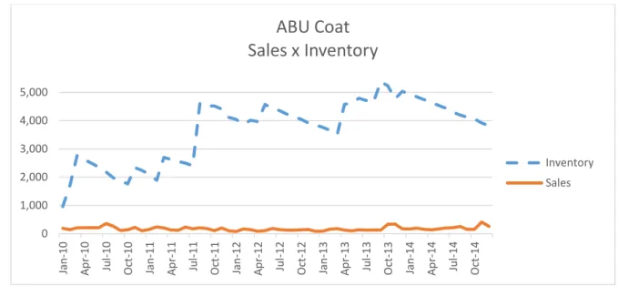
Smoothing the Bullwhip Effect in Seasonal Supply Chains
The bullwhip effect occurs when the end links of the supply chain make decisions that can over- or under-estimate the product demand, creating amplified fluctuations in inventory levels of the entire supply chain. An example of the comparison between Sales and Inventory will be seen in Chapter IV, demonstrating this phenomenon as a problem currently faced by SDS
16
and deserves special mention. In this matter, Costantino, Di Gravio, Shaban, & Tronci (2014) state that “smoothing inventory decision rules have been recognized as the most powerful approach to counteract the bullwhip effect.”
Paik & Bagchi (2007)confirmed, through computer simulation, that the bullwhip effect should be mitigated by effective information flow and channel coordination, showing the important influence of all elements of a supply chain. According to his study, “in order to control the bullwhip effect, retailers need to share the actual demand information with their partners”. However, they concluded that demand forecast updating was among the most significant variables that cause the bullwhip effect.
Long lead times lead safety stocks to increase, rising the fluctuation in demand to more significant levels. Using the exponential smoothing method, for example, continually updates future demand forecasts as new demand data become available (H. L. Lee, Padmanabhan, & Whang, 1997). Still, according to these authors, the order ‘send to the supplier’ reflects the forecasted needs for replenishing stock and necessary safety stock. With long lead times, safety stocks will naturally grow, leading to a growth in order quantities over time, as the forecasting information will become outdated.
Forecasting Role in the Supply Chain (Costantino, Di Gravio, Shaban, & Tronci, 2015)
Costantino et al., (2015)evaluated the role of forecasting in the supply chain. According to them, “although forecasting is an essential component in the inventory management of supply chains, it has been recognized as a major cause of ordering and inventory instability in supply chains”. As researchers investigate the impact of the bullwhip effect problem caused by
17
different available forecasting methods, they aim to selecting what parameters should be used under various operational conditions.
They proposed a forecasting system based on a statistical process control that can avoid frequent reactions to demand changes, counteracting the bullwhip effect, without affecting the inventory performance. This system uses two control charts integrated to decision rules to estimate the expected demand and control the inventory position. The first control chart represents a simple forecasting mechanism to predict the demand based on current variation of incoming orders/demand through a set of decision rules without over/under-reaction to demand changes. The second control chart controls the inventory position and allows order smoothing.
Their study considered the impact of the forecasting methods on the bullwhip effect investigating the effects of inventory variance in inventory costs, proving that the proper selection of forecasting methods and their parameters can help improve both ordering and inventory stability in supply chains. After all, the results confirmed the significant contribution of lead-time to the bullwhip effect and they concluded that “improved forecasting (using control charts) to control sensitivity to demand changes can reduce the contribution of longer lead-times to both the bullwhip effect and the inventory variance.”
What Experts Say
Green & Armstrong (2015) state that when it comes to forecasting, some subjects such as how to choose a method, or forecastability are always controversial issues, and usually discussed with passion. This section brings together the opinion of experts in these matters to help address basic, and yet fundamental, concerns that arose during the research.
18 Simple versus Complex Forecasting
The supra-mentioned authors affirm that, despite the common belief among scientists that scientists should make every effort in favor of simplicity, a trend toward complexity remains popular among researchers, forecasters, and clients. The evidence is that the popularity of complexity increases as its incentive is strengthened in different ways. They reveal that researchers are rewarded for publishing in highly ranked journals, which favor complexity. Forecasters can use complex methods to provide forecasts that support decision-makers’ plans. Clients may be reassured by the apparent sophistication implied by incomprehensibility. The titles and abstracts of forecasting papers in academic journals attest to the proliferation of complex methods. Not only managers, but also evenpractitioners and many researchers, are likely to struggle to comprehend typical forecasting papers (Green & Armstrong, 2015).
Simplicity in forecasting has the evident advantage of inspiring engagement by facilitating understanding. In addition, simplicity helps in detecting mistakes, significant omissions, irrelevant variables, unsupported conclusions, and even fraud. That said, there are still some reasons forecasters avoid simplicity. If the method is intuitive, reasonable, and simple, there is a fear that the client will probably not hire the forecaster, preferring, instead, to do their own forecasting. Moreover, complexity is often persuasive, even if its content is questionable. Researchers are aware that they can advance their careers by writing in a complex way. Clients might prefer (complex) forecasts that support their plans, developing complex methods that can be used to provide forecasts that support a desired outcome. It is all a matter of incentives, that is, how situations are rewarded and, in consequence, reinforced (Green & Armstrong, 2015).
In fact, incentives have been the cornerstone of human existence. An understanding of human behavior as it expresses itself in the sometimes-foggy mist of incentives is the key to
19
clearly comprehending its function. Indeed, many people in different cultures and lifestyles, who might have a natural tendency to be honest, find subtle ways of, and reasons for, cheating to move forward their position, or even to support their preferences when incentives are strong enough (Levitt & Dubner, 2006).
Simplicity avoids, or minimizes, this possible misbehavior. Although the concept of simplicity in forecasting is difficult to define, simple forecasting, for the purpose of this research, will be considered as a process that is understandable and, mostly, auditable to forecast users. Specifically, the forecasting process must be understandable with respect to methods,
representation of prior knowledge in models, relationships among the model elements, and relationships among models, forecasts, and decisions.
A good example illustrates the comparison between simple and complex forecasts: Bayes’ method has the advantage of providing another way to incorporate prior knowledge in forecasting models. However, the method has the disadvantage of being too complex for most people to understand. Experts have been unable to find evidence that Bayesian approaches yield ex ante (based on forecasts rather than actual results) forecasts that are more accurate than forecasts from simple, evidence-based methods. The Makridakis Competition (also known as M-Competition), organized by the Prof. Spyros Makridakis, aims to evaluate and compare the accuracy of different forecasting methods, including tests of Bayesian forecasting for 1 to 18 period-ahead forecasts for 997 time series. As results, forecasts from simple methods, including naïve forecasts on deseasonalized data, were more accurate than Bayesian forecasts on the basis of mean absolute percentage error (MAPE). Forecasts from the benchmark deseasonalized single exponential smoothing method reduced error by 12.4 percent. Bayesian forecasts were not included in subsequent M-Competitions. The result was that simply averaging forecasts
20
from different methods yields forecasts that reduced error, on average, by 5 percent across five studies compared to those from Bayesian approaches (Graefe, Küchenhoff, Stierle, & Riedl, 2015; S. Makridakis et al., 1982).
A simple combination of methods also provides an operational benchmark. Ahead, circumstances under which combining forecasts is beneficial in terms of results are explored.
Forecastability
As previously mentioned, popular approaches are based on comparisons of forecast accuracy with a benchmark such as the accuracy of a naïve forecast, where the actual value for a period is used as the forecast for the subsequent period (i.e. no change forecast). Metrics
employed in this approach are ratios of forecast errors from a designated model to the naïve forecast errors, and include Theil’s U statistic, the Relative Absolute Error or RAE, the Mean Absolute Percentage Error or MAPE, as well as the concept of forecast Value Added (Gilliland, 2013).
A benefit of using the naïve forecast as a benchmark is that it implicitly integrates the concept of volatility, since the naïve forecast has as much variation as the dependent variable itself. Errors associated with the naïve forecast are also probably a better predictor of
forecastability for time series purposes than, for example, the Coefficient of Variation (CoV) because they measure period-to-period variation in the data. For instance, a series in which successive observations are highly positively correlated may drift away from the sample mean for several periods, thereby contributing to a high CoV. On the other hand, the errors from a
21
naïve forecast will be relatively small because the successive observations are similar(Small & Wong, 2001).
Using a small set of easily calculated measures, such as RAE, Theil’s U, MAPE, and others, does appear to provide an objective and rational platform for constructing a set of forecast-improvement strategies tailored to a product portfolio or segment, setting the goal to maximize the overall outcome (i.e. considering the measures altogether).
Compared to similar classifications but based on conventional error metrics, these parameters bring a number of benefits, such as allowing one to assess the forecast quality by comparing cross-model same-measure results; providing a quick and simple approach for dealing with items that are forecasted poorly and where the scope for improvement does not warrant the effort (the naïve forecast); and helping to set meaningful goals, individualized to the nature of the product and the dataset behavior within a portfolio.
Combining Forecasts
Combining forecasts can reduce errors arising from faulty assumptions, bias, or mistakes in data. This procedure refers to the averaging of independent forecasts. Sometimes also
referred to as composite forecasting, this technique can be based on different datasets or different methods or both. The averaging is done using a rule that can be replicated, such as taking a simple average of the forecasts. To improve forecasting accuracy, one would combine forecasts derived from methods that differ substantially and draw from different sources of information. It is indicated, when not too costly, that it is sensible to combine forecasts from at least five
22
described. The equal weighting rule is appealing because it is simple and easy to describe, and offers a reasonable starting point. If there is good domain knowledge, or information on which method should be most accurate, it is of good sense to use different weights. Either way, the use of trimmed mean (a method of averaging that removes the largest and smallest values before calculating the mean) is desirable if you combine forecasts resulting from five or more methods. Combining forecasts is especially useful when there is uncertainty about which method is most accurate and when it is important to avoid large errors. When compared with errors of the typical individual forecast, combining reduces errors (Js Armstrong, 2001).
Another way of combining forecasts is by decomposition. This technique provides a path to simplicity for many forecasting problems. Decomposition in forecasting consists of breaking down or separating a complex problem into simpler elements before forecasting each element. Decomposition can be used with any forecasting method. Actually, the routine is most useful when different elements of the forecasting problem are forecasted by different methods, when there is valid and reliable information about each element, when the elements are subject to different causal forces, and when they are easier to predict than the whole. The separated forecasts of the elements are then combined. Decomposition is, therefore, a strategy for simplifying problems.
The relationships among the elements of the decomposed problem should be simple. Decomposition based on additive relationships is ideal. This approach is also referred to as segmentation. Decomposition based on multiplicative relationships is somewhat more complex, bearing the risk that errors will multiply. In this approach, the elements are multiplied together to obtain a forecast of the whole. Multiplicative decomposition is often useful for simplifying complex problems (Green & Armstrong, 2015).
23 Forecasting and Inventory Control
If properly related, the choice of forecasting model directly affects the amount of investment needed to support any target level of customer service. Alternative forecasting models define, each, a unique tradeoff curve between inventory investment and customer service. Careful selection of the forecasting model for an inventory system can enhance the customer service provided by a fixed investment, shifting the tradeoff curve to a higher level in parallel with its respective axis that is maintaining a constant inventory investment (Gardner, 1990).
The characteristics of the time series of inventory demands should then be analyzed in order to identify alternative forecasting models. However, since it is difficult to measure the cost of delay time in any inventory system (i.e. greater lead time), it is similarly difficult to determine where the tradeoff curve should operate (i.e. what combination between inventory investment and service level is optimal for that particular system).
Tradeoff curves between inventory investment and customer service are broadly used to support decisions in inventory control. However, it is generally accepted practice to select a specific forecasting model for an inventory and thus to establish one tradeoff curve to work with (Gardner, 1990).
Additionally, little research was found showing a relation between forecasting and
inventory decisions, yet not closely related to this study. For instance, Lee & Adam (1986) show that the size of forecast errors influences the choice of lot-sizing rules in material requirements
24
planning systems for manufacturing inventories. In distribution inventories, Eppen & Martin (1988) show that forecast errors can seriously distort projections of customer service.
After presenting the key aspects of the theories that form the framework for the investigation to be carried out under the present research, it is necessary to provide the reader with appropriate details regarding the methodology that will be employed for both data collection and analysis. This is the subject of the next chapter of this paper.
25
III. Methodology
Overview
This chapter provides details about data collection and the methodology used for analysis. Specifics of both the statistical analyses and the criteria for ordering and selecting the best results are also provided.
Data Collection
Every research project needs data to help answer questions, to understand a specific issue or totest a hypothesis. According to Patton (2014), “When one examines and judges
accomplishments and effectiveness, one is engaged in evaluation. When this examination of effectiveness is conducted systematically and empirically through careful data collection and thoughtful analysis, one is engaged in evaluation research” (Patton, 2014).
For this reason, special attention was given to this step. As the number of fields associated with each line item was considerable, it was important to determine which fields would be appropriate for this study. The selection of which fields to be collected was discussed with a software engineer, whose concern was with data integrity. Therefore, the engineer provided only audited data that was proven consistent. This gave reliability to the research, but also created constraints which prevented a more comprehensive study. As discussed in the previous chapter, for the same reasons that led to the conclusion that a simple forecast is better than a complex one, we will employ a simple data structure. The purpose is to make it as simple as possible for ease of use and understanding to ensure that the BAF Unit is able to adopt the
26
potential recommendations without undue complication in either its integration or utilization, and without hindering the effectiveness and accuracy of the final results.
Researchers can obtain their data by getting it directly from the subjects they are
studying. The resulting information is referred to as primary data. Another type of data, called secondary data, is that which has already been gathered by someone else. An advantage of using primary data is that researchers are collecting information for the specific purposes of their study. In essence, the questions the researchers ask are tailored to elicit the data that will help them with their study.
In this research, the data obtained were tailored to the research questions; that is, pulled from a large ERP database, from which only specific fields were chosen. The data needed by the present research can be considered primary, obtained directly from the organization in which the process is being analyzed. The system (ERP)’s engineer and manager have made the recorded data available.
The records were extracted from a PostgreSQL database, which is an open source object-relational database system, and wasconverted to a regular spreadsheet format, which allowed analyses to be performed. The data contained information about monthly sales and inventory over the course of five years (2010 to 2014) and the first seven months of 2015, as well as the items’ prices.
Once received, the data have been comprehensively cleansed and organized in order to be prepared for the research. In this way, all the records have been screened for any sort of
inaccuracy as well as any missing data points, in which case those data points would not be considered for this research. The analysis includes only data points for which a complete and
27
precise set of records are available. This was a necessary effort prior to the beginning of the study itself. However, as the ERP system contains its own audit, fortunately there were no records with missing information, with the exception of those in which no information was recorded for the reasons described below.
Item Selection
The selection of the items to be studied was another matter addressed with care, at the risk of jeopardizing the entire study. The first concern was to make sure that the items were picked randomly. In order to accomplish this, since there were 240 data points with sales information, a new column was inserted, and 240 random numbers were created using the “=rand” function in Microsoft Excel®. All the cells were then ordered by the column containing
the random numbers, from smallest to largest values to create a randomly ordered listing. The selection of the items occurred from the top row (with smallest random numbers) to the bottom.
Once the data was ordered, it was noticed that there were several missing data points in some of the data fields (i.e. zero sales) due to the implementation of new items, as well as item removal due to obsolescence. These missing data points differ from those observed due to lack of integrity in the data. Differently, in these cases the absence of information occurred, for instance, because an item became obsolete in January of 2012, which reduced the sales
information available to 24 months only (from January of 2010 to December of 2011). In order to keep the utility of this research to its maximum, the items with missing data points were disregarded and discarded from the selection process.
28
Tools
The next step is to find proper tools with which analyses can be run. In this particular case, MS Excel® was the primary tool utilized, as well as SAS’s statistical software solution: JMP®. Both are robust and reliable software, widely used for statistical analyses.
Methodology Used to Address the Research Questions
This section describes the methods and procedures used to address the formulated research questions.
1. What metrics are currently being utilized by the Supply Division?
To better understand the context of this study, SDS regulations were carefully examined in order to identify what categories of metrics were effective in the timeframe researched. It was then revealed that none of the documents examined disclose what types of measurements are to be used. Consequently, the information regarding this aspect of the research was obtained from the responses provided in the interview with the head of the Supply Division.
2. How can theforecasting process for uniform sales be improved in the SDS?
A proper forecast process is fundamental as a tool to optimize expenditures as well as to adjust inventory policy. Therefore, a deep analysis throughout a variety of forecast methods was necessary. Following are the methods evaluated in this research and their respective
descriptions. They were chosen for being the most commonly used by practitioners as well for the ease of use.
29 Time Series Regression
Time series regression is a statistical method for predicting a future response based on the response history (known as autoregressive dynamics) and the transfer of dynamics from relevant predictors fitting straight lines to patterns of data. In a linear regression model, the variable of interest, called “dependent” variable, is predicted from k other variables, called “independent” variables, using a linear equation. Notation wise, Y indicates the dependent variable (in this study, referring to the total monthly sales of a specific item), while X1, X2, …, Xk represent the
independent variables. Thus, the assumption is that the value of Y at time t in the dataset is determined by a linear equation:
(1)
Where β0 is known as theintercept of the model, and is the expected value of Y when all
Xs are equal tozero. βi’s are the coefficients of the variables Xi.
𝜀
𝑡 is the error term in timeperiod t. The betas together with the mean and standard deviation of the epsilons are the parameters of the model. In this research, three types of models were created in order to verify whether there were any kinds of seasonal variations or trends in the data. The first model was created using dummy variables to represent the months of the year, assigning 1 to the observed month and 0 to all others. The formula used in this case was the following:
(2)
The second model used trigonometric functions (sine and cosine) in anattempt to describe seasonal patterns. In order to test for seasonal trends, three seasonal periods (L) were
30
used, with 4-month, 2-month and 1-month periods, for the trigonometric functions, as can be seen in the following formula:
(3)
Then, an autocorrelation component was added to a simplified version of the
trigonometric function. This last factor was obtained by multiplying the previous residual (
ε
t-1)to a correlation coefficient (named
𝜙
) betweenε
t andε
t-1. As in the previous model, threeseasonal periods (L) were used, with 4-month, 2-month and 1-month periods, for the trigonometric functions. The formula for this model is the following:
(4)
(5)
Here a is assumed to be an error term (often called a random shock) with mean zero, which satisfies the constant variance, independence, and normality assumptions. Afterwards, a 4th-order polynomial model was developed in anattempt to yield a better prediction than the linear regression equation provides, with the following formula:
(6)
Decomposition
Although decomposition models are strictly an intuitive approach, they are very useful when a time series data exhibits trend, seasonal, and cyclical effects, and parameters of the time
31
series do not change over time. In practice, this method provides a forecasted point estimate “decomposing” the data into distinct components. For this study, two decomposition methods were used, namely multiplicative and additive, each one with three components: trend, seasonal, and cyclical. Following is an overview of these three components and a brief explanation of how they affect the behavior of the time series. Subsequently, the description of the models will be presented.
Trend
A trend exists when there is a long-term increase or decrease in the data. This change over time is not necessarily linear. Sometimes a trend “changing direction” will be referred to when it might go from an increasing trend to a decreasing trend or vice versa (Hyndman & Athanasopoulos, 2014).
Seasonal
Seasonality can be defined as the periodic fluctuations in a determined pattern. A
common example can be found in retail sales, which tend to peak for the Christmas season and to decline quickly after the holidays. Thus, the time series of retail sales will typically show
increasing sales from October through December, followed by rapidly declining sales in January (NIST/SEMATECH, 2013).
Cyclical
A cyclical pattern exists when data exhibit a rise-and-fall pattern that does not occur within afixed period. The duration of these fluctuations is usually at least 2 years (Hyndman & Athanasopoulos, 2014).
32
Additive and Multiplicative Methods
The multiplicative decomposition model is useful when the modeling time series displays increasing or decreasing seasonal variation. The equation for themultiplicative decomposition model is the following:
(7)
The additive decomposition model is appropriate when the time series exhibits constant seasonal variation (Bowerman et al., 2005).
The equation for additive decomposition model is the following:
(8)
Exponential Smoothing
Exponential smoothing is the most effective forecasting method when components of the time series change over time. This method weighs the actual time series values unequally, with more importance placed on the most recent data rather than earlier historical data. There are several models in exponential smoothing as expressed in (Bowerman et al., 2005), each method with a unique power to make predictions.
Simple Exponential Smoothing
This smoothing assumes that the time series has no systematic trend or seasonal
components. Nevertheless, it has a mean (or level), which may change over time. Given such a form of data, a practical approach is to take a weighted average of past values (Bowerman et al., 2005; NIST/SEMATECH, 2013).
33
The equation of thesimple exponential smoothing method is the following:
Yt = β0 +
ε
t (9)Holt’s Trend Corrected Exponential Smoothing
This method to forecast time series involves introducing a term to take into consideration the possibility of a series exhibiting some sort of trend, which can be constant or non-constant. The equation of Holt’s trend corrected exponential smoothing method is the following where the additional term represents a fixed rate of change:
Yt = (β0 + β1t) +
ε
t (10)Holt-Winters
Holt’s method can be enhanced to deal with time series containing both trend and seasonal components. The Holt-Winters method has additive and multiplicative versions.
TheAdditive Holt-Winter method is more useful for constant seasonal variation while the multiplicative Holt-Winter method is more useful for increasing seasonal variation (Bowerman et al., 2005).
The equations of the Holt-Winter methods are the following:
Additive Holt-Winters:
34
Multiplicative Holt-Winters:
Yt = (β0 + β1t) x SNt x IRt +
ε
t (12)Box-Jenkins
The Box-Jenkins method, named after the statisticians George Box and Gwilym Jenkins, applies autoregressive moving average ARMA models to find the best fit of a time series model to past values of a time series. The Box-Jenkins ARMA model is a combination of the AR (autoregressive) and MA (moving average) models. ARMA models aim to describe the autocorrelations in the data (NIST/SEMATECH, 2013).
The first step in developing a Box-Jenkins model is to determine whether the time series is stationary and if there is any significant seasonality that needs to be modeled. A stationary time series is one whose properties do not depend on the time at which the series is observed. Analyzing the data in Time Series Basic Diagnostics in JMP®, we can identify the behavior of
both theSample Autocorrelation Function (SAC) and the Sample Partial Autocorrelation Function (SPAC). A nonstationary time series will exhibit a SAC function that dies down slowly, while a stationary series will exhibit a SAC that either cuts off or dies down quickly.
Box and Jenkins recommend differencing non-stationary series one or more times to achieve stationarity. Doing so produces an ARIMA model, with the "I" standing for
"Integrated". In addition, if there was anincreasing trend in data, a pre-differencing transformation had to be performed in order to remove it using, for example, the natural logarithm.
35
If the data series were already stationary, no differencing transformation was added to the potential models. As for an initial investigation of the SAC and SPAC, when the SAC died down, and the SPAC cut off, an autoregressive model was selected. When the SAC cut off, and SPAC died down, a moving average model was selected. Finally, when both died down, a mixed model was selected. This procedure enabled initial combinations of models, as a starting point from which the determination of the best models was pursued.
ARIMA models are also capable of modeling a wide range of seasonal data. A seasonal ARIMA model is formed by including additional seasonal terms in regular ARIMA models, being necessary to determine the number of periods per season (Bowerman et al., 2005; Hyndman & Athanasopoulos, 2014; NIST/SEMATECH, 2013).
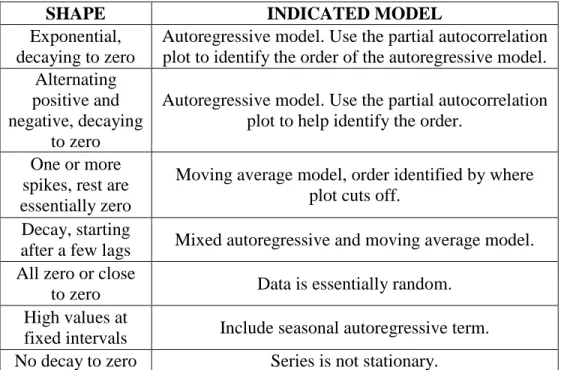
The following chart may be of some help in identifying the proper ARIMA model: (NIST/SEMATECH, 2013)
Table 1. ARIMA identification
SHAPE INDICATED MODEL
Exponential, decaying to zero
Autoregressive model. Use the partial autocorrelation plot to identify the order of the autoregressive model. Alternating
positive and negative, decaying
to zero
Autoregressive model. Use the partial autocorrelation plot to help identify the order.
One or more spikes, rest are essentially zero
Moving average model, order identified by where plot cuts off.
Decay, starting
after a few lags Mixed autoregressive and moving average model. All zero or close
to zero Data is essentially random. High values at
fixed intervals Include seasonal autoregressive term. No decay to zero Series is not stationary.
36 Choosing the methods
A template spreadsheet containing 19 models, encompassing all the methods described above, was the foundation of the data analysis. Each item, out of 240 available items, was chosen individually at a time, following the table with the randomly ordered items, from the top to the bottom.
As the sales information was plugged into the template, it was replicated to every model by linking the cells from each model tab to the original where the numbers were pasted.
Subsequently, only minor adaptations were required to calculate a forecast at each model tab as well as all other formulas to calculate the accuracy parameters (i.e. residual statistics) necessary to assess thequality of the models. The parameters will be listed and described in next section.
Finally, a tab containing a comparison chart with links to all parameters of all models was filled, and the conditional formatting tool found in MS Excel® highlighted the five best results of
each parameter among all models. From all 19 models, the five with more highlighted
parameters were selected to compose another comparison chart, with each item and its respective five best models.
The latter step was repeatedly performed, with the creation of one spreadsheet for each item evaluated, and the construction of the comparison chart with each item observed and its respective five best models. Every time one model appeared five times in the second comparison chart, this model was elected. The number of items evaluated was selected in order to yield to yield five elected models. More details of this procedure will be provided when describing the construction of the comparison chart.
37 Validity Assumptions
An important step, after having the five best models, is to verify whether the validity assumptions hold for all of them. That is, the residuals should be tested regarding normality, independence, and constant variance. Informal procedures such as diagnostic plots of residuals versus time, as pertains to time series, are recurrently used to assess the validity of these
assumptions as well as to identify possible outliers. Violation of the latter two of the
assumptions (independence and constant variance) required root data transformation or removal of outlying observations.
3. How to best assess accuracy of forecasting sales in the SDS?
A good approach to test the expectations of a model and to convincingly compare its forecasting performance against other models is to perform anout-of-sample validation. To do so, 12 data points of the sample data were withheld from the model estimation process for post validation, leaving 48 data points for model estimation (totaling 60 data points, or 5 years worth of data). The data which were notheld out (i.e. theestimation period) were used to help select the model and to estimate its parameters. Hence, the selected model is used to make predictions for the holdout data in order to perceive how accurate they are and to determine whether their residual statistics are similar to those that the model made within the sample of data that was fitted, a process called validation. Forecasts made in the estimation period are not fully "authentic" because data on both sides of each observation are used to help determine the forecast.
The model is then tested on data within the validation period, and forecasts were generated beyond the end of the estimation and validation periods. For the study’s purposes,