Dynamic Asset Allocation with Liabilities
∗
Daniel Giamouridis
†, Athanasios Sakkas
‡, Nikolaos Tessaromatis
§European Financial Management, forthcoming
Abstract
We develop an analytical solution to the dynamic multi–period portfolio choice problem of an investor with risky liabilities and time varying investment opportuni-ties. We use the model to compare the asset allocation of investors who take liabilities into account, assuming time varying returns and a multi–period setting with the asset allocation of myopic ALM investors. In the absence of regulatory constraints on asset allocation weights, there are significant gains to investors who have access to a dynamic asset allocation model with liabilities. The gains are smaller under the typical funding ratio constraints faced by pension funds.
Keywords: Strategic Asset Allocation; Dynamic Asset Allocation; Asset-Liability Man-agement, Return Predictability, Myopic Investors
JEL Classification: G11, G12, G23
∗We are grateful to the editor John Doukas and three anonymous referees for their constructive comments. Furthermore, the paper has benefited from comments by Andrew Ang, Michael Rockinger, Stephen Zeldes and participants at Fourth Joint BIS-World Bank Public Investors Conference, Washington DC 2012, at the Dauphine–Amundi Chair in Asset Management 2012 Annual Workshop, Paris 2012 and Nineteenth Inter-national Conference “Forecasting Financial Markets”, Marseille 2012. We are grateful for financial support from the “Dauphine-Amundi Chair in Asset Management”. Daniel Giamouridis also greatly acknowledges financial support from the Athens University of Economics and Business Research Center (EP-1681-01, EP-1994-01). Any remaining errors are our own responsibility.
†Daniel Giamouridis is a Director, Quantitative Solutions, Bank of America Merrill Lynch. The views expressed in this paper are his own and do not necessarily reflect those of Bank of America Merrill Lynch. Daniel Giamouridis is also affiliated with LUMS, Cass Business School, and the EDHEC-Risk Institute. This work was largely competed when Daniel Giamouridis was an Associate Professor of Finance in the Department of Accounting and Finance at Athens University of Economics and Business. E-mail address: [email protected].
‡Athanasios Sakkas is a Lecturer (Assistant Professor) in Finance, Southampton Business School, Uni-versity of Southampton, United Kingdom. E-mail address: [email protected].
§Nikolaos Tessaromatis is a Professor of Finance, EDHEC Business School and EDHEC Risk Institute, France. E-mail address: [email protected] .
1
Introduction
It is known since the work of Samuelson (1969) and Merton (1969; 1971; 1973) that long– term investors might judge risks very differently from short–term investors and hence hold different portfolios. Although Merton (1971; 1973) developed an analytical framework for understanding the portfolio demands of long–term investors, empirical implementation of his work lagged far behind due to the difficulty of solving Merton’s intertemporal model (Campbell and Viceira, 2002). The importance of liabilities in strategic asset allocation has also been long recognized by both practitioners and academics with analytical discrete– time solutions available only under static, one–period horizons. In this paper we develop an analytical solution to the dynamic multi–period portfolio choice problem of an investor under time–varying investment opportunities. We then use the model to compare the asset allocation of investors who ignore the time–varying properties of future asset risks and returns (myopic investors).
A brief taxonomy of multi–period portfolio choice solutions in an asset–only framework is provided in Jurek and Viceira(2011, JV hereafter). JV identify three types of approaches to optimal portfolio selection. First, optimal portfolios can be obtained as exact analyti-cal solutions for special cases of the multi–period portfolio choice problem in a continuous time setting (Kim and Omberg, 1996; Sorensen, 1999; Wachter, 2002; Brennan and Xia, 2002; Chacko and Viceira, 2005; Liu, 2007). Second, optimal portfolios can be determined with numerical methods (Brennan et al., 1997; Brandt, 1999; Barberis, 2000; Lynch, 2001; Dammon et al.,2001;Detemple et al.,2003;Brandt et al.,2005;Koijen et al.,2010). Third, optimal portfolios can be computed in closed-form through approximate analytical methods (Campbell and Viceira, 1999; 2001;2002, Campbell et al., 2003). JV also discuss the short-comings of these approaches and propose an analytical recursive approach which results in a closed–form solution for the dynamic multi-period portfolio choice problem.
Multi–period portfolio choice is particularly relevant for investors who invest with the objective to finance a long–term stream of liabilities. Best known examples of such investors are pension funds, foundations, and endowment funds. It is also relevant to individual investors who manage their own retirement funds or build portfolios to finance their children’s education. In this paper we study the portfolio choice problem of this type of investors, a problem that is generally referred to as Asset Liability Management (ALM hereafter).
Leibowitz (1987) andSharpe and Tint(1990) are the first papers that incorporate liabili-ties in a single period context. Since then the literature on portfolio choice in a multi–period context in the presence of liabilities parallels developments in the asset-only portfolio choice
literature. In a continuous setting Boulier et al. (1995) formulate a dynamic programming model of pension fund behavior. Sundaresan and Zapatero (1997) formulate and solve a continuous time model for the strategic asset allocation of a defined benefit pension fund taking into account the marginal productivity of the employee under a constant investment opportunity set. Rudolf and Ziemba (2004) assume time-varying investment opportunities and develop a four-fund theorem for intertemporal surplus optimization.
A second strand of the literature, closer to asset-liability modeling practice,1 uses stochas-tic programming techniques (Cari˜no et al., 1998; Cari˜no and Ziemba, 1998; Geyer and Ziemba,2008) to find optimal asset weights. A third approach is based on simulation ( Bins-bergen and Brandt,2014). These approaches are however subject to the criticisms expressed in JV in the context of asset–only portfolio choice. Stochastic programming techniques for example face the cost of tractability; the traditional numerical methods cannot handle more than a few state variables, magnifying the effects of estimation risk even further; and the ALM models carried out under a continuous time context have been mostly studied under a constant investment opportunity set.
Another strand of the ALM literature, closer in spirit to our paper, uses approximate analytical solutions and extends the asset–only models introduced by Campbell and Vi-ceira (1999; 2001;2002) and Campbell et al. (2003) by incorporating liabilities. Hoevenaars et al. (2008, HMSS hereafter) is a significant contribution in this literature. HMSS assume that an investor with risky liabilities chooses the optimal portfolio weights at the begin-ning of the investment horizon and rebalances to the initial allocation at a rebalancing time shorter than the investment horizon.Barberis(2000) describes the latter strategy as myopic rebalancing; it is myopic because the investor ignores the information available at the re-balancing time. Myopic investors maintain the initial static solution, through rere-balancing, until the end of the horizon. In contrast, dynamic investors follow a dynamic investment strategy where the portfolio weights take into account changes in the investor’s investment opportunity set. Using the myopic asset-liability model (M–ALM thereafter), HMSS find significant differences in the portfolio allocations of investors who ignore liabilities.
Our principal contribution in this paper is that we develop a model which results in a closed–form solution for the dynamic multi–period portfolio choice problem in the presence of liabilities (D–ALM thereafter). Our model nests the asset–only model of JV. It is analytically tractable and hence allows the study and interpretation of factors affecting optimal portfolio
1ALM based on stochastic programming and used in practice include the Russel–Yasuda Kasai model described in Cari˜no et al. (1998) and the Towers Perrin–Tillinghast ALM approach presented in Mulvey et al.(2000).
choice in an ALM framework. The model we propose can accommodate any number of assets and state variables. To develop the proposed model we build on JV and HMSS. Our representative investor is endowed with power utility over the ratio of assets and liabilities, as opposed to over assets only, at a fixed horizon; she can invest in many risky and a riskless asset. The investment opportunity set is time–varying and captures the variation in risk premia, interest rates, and the state variables. The optimal investment policy that we derive has a simple structure; it is comprised of myopic and intertemporal hedging terms. The novel feature of our model is that we show analytically how the intertemporal hedging demand – which appears in the asset–only multi–period portfolio choice literature – is also driven by the correlation between the innovations of liabilities and the innovations in the changes of the state variables.
In our empirical investigation we take into account practical considerations. We incor-porate short–sales or borrowing constraints, as in Brandt et al. (2009). We also consider a regulatory environment in which pension funds face minimum and maximum funding ratio constraints. The model we develop allows us to study the structure of optimal portfolios as well as the utility implications associated with holding these portfolios. In this respect, we provide new empirical insights that are useful both for ALM researchers but also for the practice of ALM. Furthermore, with the incorporation of inflation–indexed bonds in the list of potential investment assets, we are able to study the allocation to inflation–indexed bonds in the portfolios of long–term ALM investors. Campbell and Viceira (2002) argue that inflation–indexed bonds are important for long–term asset–only investors since both bonds and (rolling) short-term bills are subject to real interest rate variations over time. Inflation-indexed bonds are even more important for ALM investor with inflation sensitive liabilities.
Our empirical results can be summarized as follows. We find that optimal portfolios obtained using the D–ALM are different in many respects with optimal portfolios obtained for myopic ALM investors. Myopic investors hold portfolios which contain more equity and inflation-indexed bonds than D–ALM investors. The higher allocation to equities and indexed bonds is at the expense of a lower position in nominal bonds. This conclusion does not change when we impose short-sell or funding ratio constraints.
The differences in the composition of D–ALM optimal portfolios and M–ALM optimal portfolios have significant utility implications. In particular, we find that a M–ALM investor suffers large utility losses relative to the portfolios suggested by the D–ALM. The losses are increasing in the length of the investment horizon and decreasing in the degree of relative risk
aversion. The economic benefits of the D–ALM over the M–ALM strategy reflect the benefits from pursuing a dynamic investment strategy that exploits information about asset time-varying returns and risks and hedging abilities. The D–ALM provides the optimal strategic and tactical asset allocation portfolios for investors with multi–period horizons and liabilities. A moderate risk aversion M–ALM investor, assuming leverage is not allowed, is prepared to pay up to 1.14% per month to gain access to the D–ALM. The maximum management fee increases for more conservative investors. In the presence of minimum and maximum funding ratio constraints, like those faced by defined benefit pension funds in practice, the utility losses are smaller but remain significant. Imposing tight funding constraints reduces but does not eliminate the benefits from hedging dynamically the investment opportunity set and liabilities.
Comparing the composition of optimal portfolios obtained with the proposed model with optimal portfolios obtained for AM investors (as in JV), we find that the two approaches generate different asset allocations. While equity allocations are similar, nominal bond al-locations tend to be lower for ALM investors compared to the alal-locations of AM investors. In contrast, ALM portfolios contain substantially more inflation–indexed bonds than AM portfolios, reflecting the liability hedging properties of inflation–indexed bonds. The dif-ferences in the composition of the optimal portfolios between the two approaches translate to substantial losses for a moderate and highly risk averse AM investor in the presence of liabilities which increase as the investment horizon increases.
The rest of the paper is organized as follows. Section 2 specifies the investment setting and derives the closed–form expression of asset weights for ALM optimal portfolios. Section3 introduces the data and presents the results of the estimation of the dynamics of the available investment opportunities. Section 4 examines the structure of optimal portfolios obtained through the D–ALM and M–ALM strategies. Section 5 investigates the utility implications associated with the M–ALM strategy and Section 6 examines the implications for asset allocation and utility of funding ratio constraints and alternative liability benchmarks and we also benchmark key empirical results to JV. Finally, Section7 concludes. The Appendix provides a detailed derivation of all the analytical results in the paper.
2
The setting
In this Section we outline the details of the dynamics of the investment opportunities that are available to our investor; an investor that determines her holdings such that she will be able
to finance a long–term stream of liabilities. We then define her multi–period portfolio choice problem. Finally we apply an analytical recursive approach which results in a closed-form solution and hence a closed–form expression for the optimal investment policy.
2.1
The dynamics of the available investment opportunities
We model the dynamics of the available investment opportunities through a VAR(1) spec-ification as in Campbell and Viceira (2002).2 We augment the investment opportunity set
with the investor’s liabilities. Hence, our economy is one where expected returns, liabilities, and interest rates are time-varying and are jointly determined through:
zt+1 =Φ0+Φ1zt+vt+1 (1)
In equation (1), zt+1 denotes a column vector whose elements are the log returns on the asset classes we consider as potential investments, the liabilities (an appropriate proxy is considered as we discuss below), and the values of the state variables at time t + 1. Φ0 is a vector of intercepts, Φ1 is a square coefficient matrix, and vt+1 is a vector of zero mean innovation process. We assume these innovations are homoskedastic and normally distributed, that is vt+1
i.i.d.
∼ N(0,Συ).Chacko and Viceira (2005) argue that the persistence
and volatility of risk do not affect the portfolio rule of long-term investors. For ease of reference we can re-write the vector zt+1 as:
zt+1 = rtb,t+1 xA,t+1 xL,t+1 st+1 (2)
where rtb,t+1 denotes the log real return on the T-bill; xA,t+1 is a vector of log real excess returns on all other assets (considered as potential investments) with respect to the real return on T–bills, that is xA,t+1 = rA,t+1−rtb,t+1 ; xL,t+1 is a vector of log excess returns on the liabilities with respect to the real return on T–bills, that is xL,t+1 =rL,t+1−rtb,t+1 ;
2Campbell and Viceira(2002) provide a comprehensive review of the applications of the VAR specification for modelling the intertemporal behaviour of asset returns and their application to the portfolio choice problem. Much of the dynamic portfolio choice literature utilizes a VAR(1) as a compromise between the size of the model and the estimation error. Other modelling approaches combine dynamic asset allocation with a regime–switching model which is beyond the scope of the paper (see for example Ang and Bekaert
and, finally, st+1 is a vector with the realizations of the state variables that are believed to be important in determining asset prices. All returns are defined in real terms in excess of realized inflationπt. We can also write the variance–covariance matrix of the shocksvt+1 as:
Συ = σtb2 σ>tbA σ>tbL σ>tbS σtbA ΣAA σ>AL Σ > AS σtbL σAL σL2 σ>LS σtbS ΣAS σLS ΣSS (3)
The elements on the main diagonal are σtb2, the variance of the real return on the T-bill;ΣAA, the variance–covariance matrix of unexpected excess asset returns;σ2L, the variance
of the unexpected excess liabilities returns; and ΣSS, the variance-covariance matrix of the
shocks to the state variables. The off-diagonal elements are the covariances of the real return on the T–bill with excess returns on all other assets and liabilities,σtbAandσtbL, respectively;
the covariances of the real return on the T-bill and shocks to the state variables, σtbS; the covariance of assets and liabilities σAL; and the covariances of excess returns and liabilities with shocks to the state variables ΣAS and σLS, respectively.
2.2
The investor’s optimization problem
In the multi–period portfolio choice problem the investor targets a specific payoff at a given investment horizon and takes into account the changes in the anticipations for the distribu-tion of asset returns or relevant factors. Investors that determine their holdings such that they will be able to finance a long–term stream of liabilities are concerned with the value of their assets relative to the value of their liabilities; not the absolute value of their assets. For example, a pension fund, should ensure that it covers future pension payments with their assets, without the need for further contribution. Therefore, within an ALM context, the investor’s utility optimization problem is expressed with respect to her funding ratio Ft at
time t. The funding ratio is defined as the ratio of Assets (A) over Liabilities (L), i.e. the funding ratio at time t is Ft = At/Lt.3 The investor is assumed to have Constant Relative
Risk Aversion (CRRA hereafter) preferences on the terminal funding ratio. We assume that at each decision point the investor’s liability has a constant maturity.4 Hence we specify her
3 Leibowitz et al. (1994), McCarthy and Miles (2013), Binsbergen and Brandt (2014), and HMSS are studies, among others in the ALM literature, that seek optimal asset allocations through maximization of the investor’s funding ratio utility.
4For pension funds that means that the fund is closed to new entrants and that the value of contributions is equal to the present value of the new liabilities created. Like HMSS we assume that the pension fund is in
utility function at the terminal datet+K as: u(Ft+K) = ( 1 1−γF 1−γ t+K f or γ 6= 1 log(Ft+K) f or γ = 1 (4)
where γ is the relative risk aversion coefficient. We follow JV in that we assume that the investor chooses the portfolio weights αALM,t+K−τ between times t and t+K −1 so as to
maximize the expected value of the utility function, that is:
maxEt[u(Ft+K)] (5)
which we can re-write through equation (4) as: {αALM,t+K−τ}ττ=1=K = argmax
1
1−γEt[exp{(1−γ)rF,t→t+K}],when γ 6= 1 (6)
{αALM,t+K−τ}ττ=1=K = argmaxEt[rF,t→t+K],whenγ = 1 (7)
The subscript in the portfolio weight vectorαALM,t+K−τ in equations (6) and (7) corresponds
to the time at which the portfolio weights are chosen and the superscript denotes the time remaining. rF,t→t+K denotes the funding ratio log-return between time t and t+K , that
is the logarithmic return of the asset portfolio rA,t→t+K minus the logarithmic real return
on the liabilities rL,t→t+K . To compute rF,t+1, which is rF,t+1 = rA,t+1 −rL,t+1 we use a standard log-linear approximation ofrA,t+1 following Campbell et al.(2003) and JV among others. Campbell et al. (2003) and JV use the following log–linear approximation to the portfolio return rA,t+1, rA,t+1 ≈ α>AM,t xA,+1+12σ2A
− 1 2α
>
AM,tΣAAαAM,t +rtb,t+1, where
rtb,t+1 denotes the T–bill rate, αAM,t the allocation to risky assets and σ2A is the vector
consisting of the diagonal elements of the variance covariance matrix of the risky assets. The log return on the wealth portfolio is a linear combination of the excess returns, volatilities and covariances on the benchmark asset (i.e. T–bill rate) and the risky assets. Campbell et al.(2003) argue that the log–linear approximation torA,t+1 becomes increasingly accurate as the frequency of portfolio rebalancing increases and it is exact in the continuous limit. We subtract the return on liabilities (rL) from both sides of the equation. Hence, the log–linear
approximation to the log funding ratio return rF,t+1 can be expressed as: rF,t+1 ≈α>ALM,t xA,t+1+ 1 2σ 2 A − 1 2α > ALM,tΣAAαALM,t−xL,t+1 (8) where σ2
A is the vector consisting of the diagonal elements of ΣAA. In equation (8) the
benchmark asset is the investor’s liability – hence the negative sign – whereas in Campbell et al. (2003) and JV the benchmark asset is the T–bill rate.
2.3
The optimal investment policy
We solve for the optimal dynamic optimization problem based on standard backwards re-cursion as in JV. The first step of this process involves the derivation of the portfolio rule (policy function) and the corresponding value function in the last period. In the second step we define the portfolio rule of the period preceding the last period as a function of the value and the policy function coefficients from the terminal period. The last step involves iterating this relationship to derive the solution to the ALM multi–period portfolio choice with dynamic rebalancing.
More specifically in the first step we define the optimal portfolio policy of an investor with one period remaining to the terminal date t+K :
α(1)ALM,t+K−1 = 1 γΣ −1 AA Et+K−1[rA,t+K −rtb,t+K] + 1 2σ 2 A−(1−γ)σAL (9) where Et+K−1[rA,t+K−rtb,t+K] =HA(Φ0+Φ1zt+K−1) (10) andHAis a matrix operator that selects the rows corresponding to the vector of asset excess
returns xA from the target matrix.
Equation (9) is the myopic or one–period mean–variance efficient portfolio rule. The op-timal myopic portfolio has two components. Aspeculativecomponent, which is the tangency portfolio, usually referred to as the Performance Seeking Portfolio (PSP):
1 γΣ −1 AA Et+K−1[rA,t+K−rtb,t+K] + 1 2σ 2 A (11)
a hedging component, the Liability Hedge Portfolio (LHP):5 1− 1 γ Σ−AA1σAL (12)
which depends only on the variance–covariance matrix of asset returns and the covariance of asset returns with the liabilities.
Under the assumption of time-varying expected returns and homoskedasticity, the PSP changes with the investment opportunities in contrast to the LHP which remains constant across the investment opportunities. Log utility investors (γ = 1) hold only the PSP, while highly risk adverse investors (γ → ∞) hold only the LHP.
In the second and third steps we derive the solution to the ALM multi–period portfolio choice with dynamic rebalancing (see ??):
α(ALM,tτ) +K−τ = 1γΣ−AA1 Et+K−τ[rA,t+K−τ+1−rtb,t+K−τ+1] +12σ2A−(1−γ)σAL −1− 1 γ Σ−AA1ΣA B(τ−1) > ALM,1 + BALM,(τ−1)2+B(τ−1) > ALM,2 Et+K−τ[zt+K−τ+1] (13) where ΣA = h σtbA ΣAA σ>AL Σ>AS i and B(τ−1) > ALM,1, B (τ−1) ALM,2 and B (τ−1)>
ALM,2 are functions of the remaining investment period, the coefficient risk aversion γ and the coefficients of the VAR system. The multi–period optimal portfolio obtained through equation (13) has two components too. The first component:
1 γΣ −1 AA Et+K−τ[rA,t+K−τ+1−rtb,t+K−τ+1] + 1 2σ 2 A−(1−γ)σAL (14)
is the myopic component given by equation (9). The optimal myopic portfolio in equation (14) combines the PSP, i.e. equation (11), and the LHP, i.e. equation (12). It is a function of one–period expected returns and the conditional variance–covariance matrix of one–period returns of assets and liabilities.
The second component:
1− 1 γ Σ−AA1ΣA B(τ−1) > ALM,1 + BALM,(τ−1)2+B(τ−1) > ALM,2 Et+K−τ[zt+K−τ+1] (15)
is the ALM–intertemporal hedging component. The ALM–intertemporal hedging component
is the unique element of our model. It differs from the intertemporal hedging component which was first introduced byMerton(1969;1971;1973) under an AM context. It is the prod-uct of two factors. The first termΣ−AA1ΣAcaptures the ability of assets to hedge changes in the
investment opportunities, taking also into account the instantaneous correlation with the lia-bilities, a correlation that it is not considered in the intertemporal hedging component of Mer-ton. The second term,1− 1
γ Σ−AA1ΣA B(τ−1) > ALM,1 + BALM,(τ−1)2+B(τ−1) > ALM,2 Et+K−τ[zt+K−τ+1] , captures the effect of changes in investment opportunities on the investor’s marginal utility. It corresponds to the ratio of the cross–partial derivative of the value function with respect to funding ratio and the vector of state variables, and, the product of funding ratio and the second derivative of the value function with respect to funding ratio.
For simplicity we can rewrite equation (13) as:
α(ALM,tτ) +K−τ =A(ALM,τ) 0+A(ALM,τ) 1zt+K−τ (16)
where A(ALM,τ) 0 and A(ALM,τ) 1 can be deduced from equation (13). Equation (16) shows that the solution to the ALM multi–period portfolio choice with dynamic rebalancing is an affine function of the vector of state variables zt+K−τ. This suggests that as in JV A
(τ)
ALM,0 and
A(ALM,τ) 1 (and hence also the optimal investment policy), depend on the time remaining to the terminal horizon date but are themselves independent of time.
Some special cases of equation (16) deserve further attention. We show in ?? that for a log utility investor (γ = 1) or a constant investment opportunity set (Φ1 = 0) the dynamic portfolio choice problem converges to a myopic portfolio choice problem. In addition, an infinite risk averse investor (γ → ∞) invests in the least–risky portfolio which is independent of the vector of unconditional expected returns; under a constant investment opportunity set the infinite risk averse investor holds the LHP.
One limitation of analytical approaches is that they cannot accommodate portfolio con-straints explicitly. In our empirical analysis we adopt Brandt et al. (2009). We impose short–sales constraints by truncating the negative portfolio weights in equation (16) at zero and renormalizing the optimal weights in order to sum to one, that is:
α+ALM,i,t= max [0,αALM,i,t]
PN
j=1max [0,αALM,j,t]
3
Data and model calibration
In this Section, we discuss the investment opportunity set we consider and the data we use in our empirical analysis. We additionally discuss the estimation procedure and the estimates of the fitted dynamics of the available investment opportunities. Finally, we present the term structure of risk of the asset classes as well as the term structure of the correlation of the asset classes with liabilities.
3.1
Assets, liabilities and state variables
The framework we propose is a general one and hence its empirical implications can be investigated with any number of asset classes and state variables. In the empirical imple-mentation of the model we present later we assume that the investor has access to equities, nominal bonds, cash and inflation-linked bonds.
The empirical implementation of the D–ALM portfolio choice problem also requires a measure of investors’ liabilities. The liability structure however depends on the particular circumstances of the investor. From an individual investor’s perspective for example the retirement portfolio’s objective is to maintain the investor’s standard of living after retire-ment. We can therefore assume that the investor aims for a positive real return and hence that her “liability” is similar to an inflation-indexed bond. From the perspective of a de-fined benefit pension fund we can assume that the age cohorts and vested pension rights per cohort are constant over time and future benefits are fully indexed to inflation. We also assume that future contributions equal the present value of the liability created. Under these conditions the liabilities of the pension fund could be proxied by the returns of an inflation–indexed portfolio with duration equal to the duration of the pension’s liabilities. The choice of inflation–indexed bonds as a proxy for liabilities allows us to gain empirical insights with the proposed model in the context of a very general, yet representative, type of liability. The drawback of this choice is that risks that may affect the dynamics of liabilities, such as actuarial, longevity and demographic risks, are not taken into account. Future work should focus exclusively on the integration of such risks with market risks in the strategic asset allocation problem (see, e.g. Bisetti et al. (2016)).
When index–linked bonds do not exist or there is a short history of indexed bond prices, index–linked bond prices could be estimated from nominal bond yields. This is the approach taken in studies based on US data where indexed–bonds (TIPS) first appeared in 1998. Before the introduction of TIPS, Campbell and Shiller (1997) use short–term real interest
rates and the expectations theory of the term structure to create a hypothetical series for index–linked bond returns. Kothari and Shanken (2004), and HMSS use the observed yield on long term nominal bonds and assumptions about expected inflation and the inflation premium to calculate real yields for indexed bonds. This approach generates a long history of data which however it is subject to estimation errors.6 To isolate potential estimation
errors of this kind, we use information about inflation–indexed bonds prices and yields from the UK. The first indexed–linked bond was introduced in the UK in the budget of 1981 and the first bond was traded in 1982. Prices and yields are available since then providing the longest history of real yields compared to other developed markets.
We source data from DataStream. All data are in pounds. Stock returns are represented by the UK Datastream value-weighted stock index (including distributions). We proxy for nominal bonds through the DataStream’s UK twenty-year constant maturity bond, for inflation-indexed bonds through the FTSE British Government Index Linked All Maturities index and for the cash we use the UK interbank 3–months rate.
As proxies of the state variables that determine the dynamics of stock excess returns, bond excess returns and interest rates as per equation (1) we use a set of common variables used in previous research.7 These include the dividend–price ratio (DY) on the UK value– weighted stock index; the short–term nominal interest rate; the term spread (the difference between the ten–year treasury constant maturity rate and the three–month T–Bill rate) and the ex–post real rate of return on a 3 month Treasury bill (the difference between the return on the three-month UK Treasury bills and the inflation rate). We consider the ex–post real rate as the real return on an investable asset (cash) as well as a state variable. JV find that the utility losses of dynamic investors who do not rebalance their portfolios on a monthly basis increase as the rebalancing frequency decreases. We therefore base our analysis on monthly data covering the period January 1982 to December 2014.
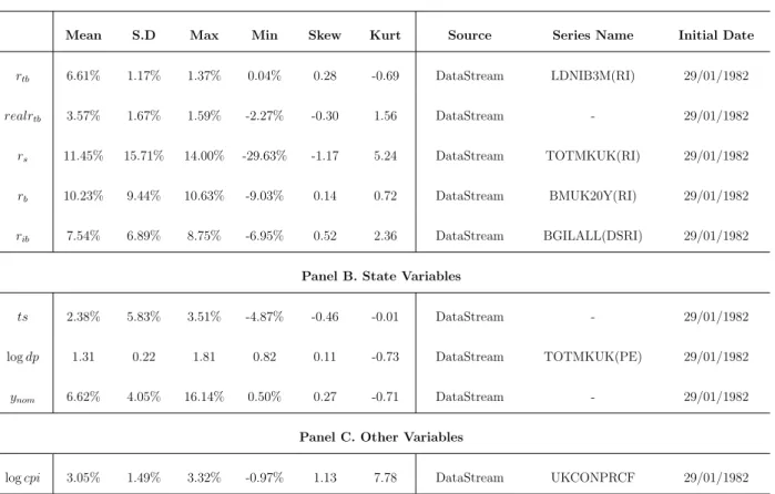
Table 1presents the descriptive statistics of monthly nominal returns of the asset classes and state variables included in the VAR model for the entire period. The returns of the assets classes are expressed in nominal terms. The mean and the standard deviation are annualized. Equities achieved the highest annual nominal mean return (11.45%), albeit
6Campbell and Viceira(2009) study the differences between synthetic and actual index-linked returns. They find that synthetic yields are lower on average and less volatile compared to actual ones. Additionally, they observe a correlation equal to 0.70 for the period 1982–2008.
7Key papers in this literature are Campbell and Shiller (1988; 1991; 1998; 2005),Fama and Schwert (1977), Campbell(1987),Glosten et al.(1993),Fama and Bliss (1987), Fama and French (1989), Campbell et al.(2003),Campbell and Viceira(2005). The evidence on predictability are controversial (Bossaerts and Hillion,1999;Welch and Goyal,2008).
only slightly higher than the return of nominal bonds (10.23%). During the period, the realized equity premium vis a vis nominal long-term bonds were significantly lower to the long-term historical average. Inflation–indexed bonds had a return of 7.54% per annum, lower than equities and nominal bonds. Equity returns are negatively skewed and have the highest kurtosis among all asset classes. Volatility is much higher for stocks (15.71%) than for nominal bonds (9.44%) and real bonds (6.89%); nominal bonds are more volatile than indexed bonds.
3.2
VAR estimates and term structure of risk and correlation
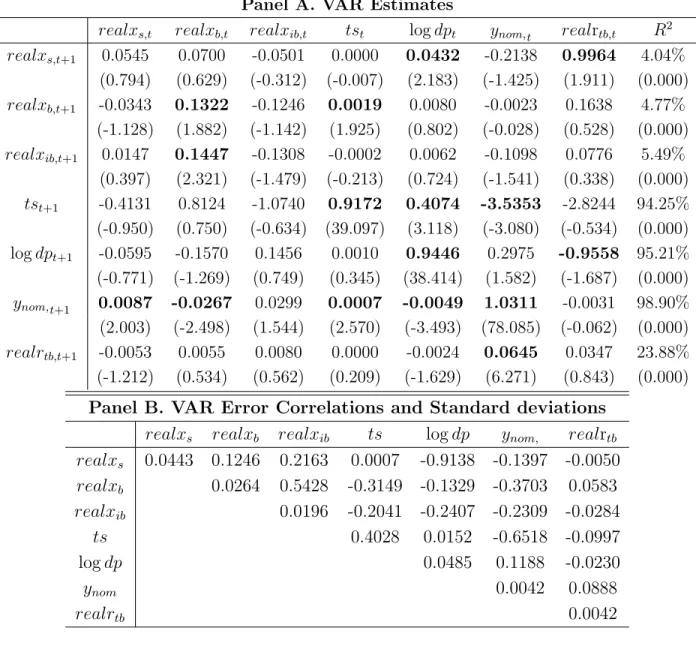
We present the estimates of the parameters of equation (1) in Table 2.8 Panel A of Table 2 shows the slope coefficient parameter estimates of the VAR system. Panel B of Table 2 reports the standard deviations (in the diagonal) and the correlations (off-diagonal elements) of the innovations. As in previous studies, we find that excess stock returns are predictable by the dividend–price ratio and the short term real interest rate. For the excess nominal bond return its lagged return and the term spread are important, statistically, variables that predict future bond premia. A high spread and nominal bond return are associated with higher future nominal bond returns. The short term nominal yield is a strong predictors of the real interest rate. Finally, an increase in short term nominal interest rate is associated with lower returns for indexed bonds and by implication liabilities. TheR2 for the equations of the excess market and bond as well as the liabilities returns are fairly low but typical of estimates reported in the predictability literature.Campbell and Thompson (2008) argue that whileR2 increases at lower frequencies, even low values are associated with economically meaningful outcomes. Evidence in Rapach and Zhou (2013) for stock returns suggests that even a small degree of predictability can produce substantial utility gains.
The dynamics of the state variables we document are consistent with the empirical lit-erature (Brennan et al., 1997; Campbell and Viceira, 2002; Campbell et al., 2003). The coefficients of the dividend–price ratio, the nominal short interest rate, and the term spread suggest persistent autoregressive processes. The maximal eigenvalue of the coefficient ma-trix equals 0.9933, implying that the VAR is stationary with a half-life of about 7 years. The system is stable, but close to being integrated of order one. We do not make any ad-justment in the coefficient estimates of the VAR system for possible biases related to near
8Incorporating parameter and model uncertainty is beyond the scope of this paper but results in
Hoeve-naars et al.(2014) suggest that taking this uncertainty into account will increase the allocation to nominal bonds at the expense of equity allocation as the investment horizon increases.
non-stationarity of some time series (Brennan et al., 1997; Campbell and Viceira, 2002; Campbell et al., 2003). Campbell and Yogo (2006) argue that the processes for the state variables are highly persistent rather than unit-root processes.
The results presented in Panel B of Table2suggest that the innovations to the dividend– price ratio are negatively correlated with unexpected excess returns on equities. The negative correlation between shocks to the dividend–price ratio and shocks to stock excess returns combined with the positive relation between the dividend–price ratio and subsequent stock returns is consistent with mean reversion in stock prices. A decrease in the dividend–price ratio following an increase in stock prices is associated with high returns today but followed by higher expected returns in the future. Mean reversion in stock prices is also indicated by the positive relation between the short term real rate and future stock returns and the negative correlation between shocks to returns and interest rates. The term spread reinforces the mean reversion of stock returns. The most important variables for nominal bond excess returns are the term spread and the short term real rate. The effects of these variables on the future behavior of bond returns are opposite. The term spread predicts positively future bond returns while shocks to the term spread and bond returns are negatively correlated. The combined effect is consistent with mean reversion in bond prices. In contrast, the positive relation between bond returns and real rates and the positive correlation between innovations to the real rate and bond returns suggest mean aversion. Which effect dominates is an empirical issue. The VAR estimates for the real interest rate are consistent with findings in the literature (seeCampbell and Viceira(2005) and HMSS) and are indicative of increased risk with the horizon (mean aversion). Finally, future real bond returns and hence liabilities are positively related with short term real rates and negatively related to short term nominal rates. Shocks to indexed–bond returns are strongly negatively correlated with shocks to the nominal short yield.
The VAR model provides a convenient framework to calculate the conditional term struc-ture of volatilities and correlation of asset returns, assuming that the VAR model capstruc-tures correctly the dynamics of asset returns.
As shown in the Appendix, Figure B1 presents the term structure of risk of T-bills, equities, nominal and real bonds/liabilities. We find that equities are less risky in the long run, whilst nominal bond return volatility exhibits mild mean aversion as in Campbell and Viceira (2005). T–bills are riskier in the long run. Liability returns, as proxied by real bond returns, exhibit also a mean averting behavior, implying that liability risk is higher in the long run. The latter magnifies the importance of considering liabilities in a dynamic asset
allocation policy.
Figure B2 shows the correlation structure of asset returns with real returns on liabilities. In the short-term, equities are weakly correlated with liabilities; in the medium and long term the correlation declines to about zero. Real returns on nominal bonds with constant maturity are positively correlated with returns on liabilities at all investment horizons; at short horizons the correlation is about 55% and increases in the long run to 80%.9Finally,
T–bills are a bad liability hedge at all investment horizons, due to their negative correlation with liabilities.
4
Portfolio allocations in the presence of liabilities
In this Section we provide an investigation of the D–ALM implications for portfolio manage-ment. We are interested in particular at the differences between the optimal mean-variance portfolios generated by the dynamic asset liability model (D–ALM) and the optimal port-folios generated by a single period mean-variance approach that incorporates liabilities (the M–ALM). For each model, we derive two sets of optimal weights. One is derived through equation (16), and a second set of optimal weights is derived with short-selling constraints through equation (17).To compute the allocations we assume a long–term expected real return on the T-bill equal to 2% per year, a return on the value-weighted stock index of 7% per year, a return on the nominal bond index of 4% per year, and a return on the real bond of 3.5% per year. We believe that these premia represent a reasonable compromise between historical averages (based on data covering the period January 1982 to December 2014) and historical/forward-looking estimates reported inDimson et al.(2008;2011).Campbell and Viceira(2002) make similar assumptions, i.e. riskless real interest rate of 2% per year, equity premium of 4% per year. We also assume an inflation risk premium of 0.5% based on Kothari and Shanken (2004). To generate the asset allocation weights we use the long term expected returns and the VAR model to generate time varying forecasts of returns, combined them with equation (16) to get one set of asset allocation weights per future time period for the dynamic asset-liability investor. In particular, we impose long–term views on asset returns and risk premia by adjusting the constant term of the proposed VAR model. The constant term can be derived as Φ∗0 = (I−Φ1)µ, whereµis a (n×1) vector containing the long–term means of
9Kothari and Shanken(2004) find that the correlation between nominal and real bonds is 0.53 and 0.58 when nominal and real returns are used respectively.
the risk premia and state variables. Hence, the transformed constant Φ∗0 and the estimated coefficient matrix Φ1 (shown in Table 2) are used to generate the asset allocation weights.
Finally, the state variables are at their long run historical mean.
For both the M–ALM and the D–ALM cases we assume that portfolio decisions are made monthly. The main difference between M–ALM and D–ALM is that under the dynamic asset-liability setting the optimal weights today depend on the time–varying expectations of returns and risks. In contrast, under M–ALM portfolio weights today take into account the expected return, volatility and correlations to the horizon but assumes that the investor does not take into account monthly time varying opportunities. Dynamic investors take into account not only the short–term return and risk characteristics of assets but also their ability to hedge liabilities and provide a hedge against changes in the opportunity set.
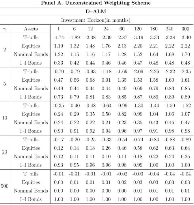
Table 3 reports asset class weights for the D–ALM and M–ALM investor for different investment horizons (from 1 to 300 months) and different attitudes towards risk (different risk aversion parameters). Panel A of Table 3 tabulates the allocations for portfolios with no constraints on portfolio weights. Note that for the one month horizon both dynamic and myopic investors hold exactly the same portfolios. For reasonable risk aversion parameters, both myopic and dynamic investors would borrow to invest in the risky assets. The negative weight of cash reflects the increased volatility and the negative correlation of short term interest rates with liabilities.
Low and moderate risk averse dynamic investors invest in general less in equities than myopic investors. In contrast, dynamic investors invest more in nominal bonds for different risk aversion parameter and horizons. The allocation to inflation–indexed bonds tend to be higher for dynamic rather than myopic investors as the horizon increases.
For the myopic investor, an increase in the investment horizon is associated with increased demand for equities and nominal bonds and decreased demand for index linked bonds. For the myopic investor asset allocation weights depend on expected returns, risks and the corre-lation between asset and liabilities. The increasing weight of equities as the horizon lengthens reflects the decrease in equity volatility due to mean reversion of stock prices. The increasing weight in nominal bonds reflects two opposing forces: the good liability hedging properties of nominal bonds and the increased volatility of bonds at longer horizons. More conservative investors tend to put a large part of their portfolio to indexed bonds at the expense of both equities and nominal bonds, assets that are only partial hedges against liabilities.
Dynamic investors, in addition to their concerns to match liabilities, also take into account the predictability of asset returns. The main differences in portfolio weights compared to
the myopic investor is that as the investment horizon increases, the dynamic investor invests more in equities and nominal bonds financed by more borrowing than the myopic investor. The additional weight in bonds and equities reflects the ability of nominal bonds and stocks to hedge changes in the opportunity set. Indexed bond weights are almost stable at all investment horizons.
To gain further insights on the drivers of the differences in portfolio allocations and the role of state variables in their variation we turn our eye to Tables 2 and 3. For equities the most important driver of equity allocations is the dividend yield. An increase in the market dividend yield is associated with an increase in expected equity returns and an increase in the intertemporal hedging demand for equities. For nominal bonds, a negative innovation in the term spread reduces expected returns and increases the hedging demand for bonds
Panel B in Table 3 shows optimal weights for dynamic and myopic investors assuming borrowing is not allowed. Borrowing to invest may be unrealistic for most investors and in particular for pension funds. We observe that short–selling constraints have a significant impact on portfolio allocations. Both dynamic and myopic investors increase the weight of stocks as the horizon increases. Equities are attractive because volatility falls. For example dynamic investors with risk aversion equal to 5 increase the equity weights from 28% when the investment horizon is one month to 48% when the horizon is 300 months. For the myopic investors equity holdings increase from 28% to 63%. Myopic investors assume a lower volatility as a result of equity mean reversion than dynamic investors who use the full term structure of volatility estimates and therefore use on average higher volatility estimates in the asset allocation construction process.
Myopic investors with moderate risk aversion (γ = 5) allocate 29% in nominal bonds in the short term and the weight decrease to 17% for long term investors. Similarly, dynamic investors start with 29% at the monthly horizon and invest 25% at the 300 month horizon. The decrease in bond holdings as the horizon increases reflects the mean aversion properties of nominal bond prices discussed in Section 3. Myopic investors invest less than dynamic investors since they use, on average, a higher volatility estimate (mean aversion) in the asset allocation process. The asset allocation weight of indexed bonds is slightly over 40% and decreases to 20% at 25 years investment horizon. More conservative investors (higher risk aversion parameters) switch from equities and nominal bonds to indexed bonds as expected. The fall in bond portfolio weights as the horizon increases reflects the mean averting prop-erties of nominal bonds whilst the increase in equity weights reflects the mean reversion properties of stocks.
Overall, the evidence presented in this Section suggests that dynamic optimal portfolios are different to myopic optimal portfolios primarily in their allocations to nominal bonds (for all investors and moderate to long investment horizons). Dynamic investors tend to allocate less in equities and more in indexed bonds. We study the economic implications of these differences in the next Section.
5
The economic value of dynamic rebalancing
The empirical results presented above suggest that a dynamic ALM investor holds a different portfolio compared with the portfolio held by a myopic ALM investor. In this Section we investigate the utility implications associated with these differences.
We measure the economic implications of different allocations through the certainty equivalent (CE hereafter) of the funding ratio Ft, which is defined as follows:
FCE =u−1
EhuFfT i
(18) To compute the CE, we first simulate 10,000 paths of the VAR system for the monthly fre-quency. We compute the optimal asset allocation policy through equation (16), the realized terminal funding ratio, and the realized utility of the terminal funding ratio along each path. Finally, we compute the average realized utility across paths and based on equation (18) we obtain the CE. The value function with periods remaining is:
max 1 1−γEt+K−τ " exp ( (1−γ) τ X i=1 rF,t+K−τ α(ALM,tτ+1−i+)K+i−(τ+1) )# (19)
The utility loss of a myopic investor who does not use the D–ALM is calculated as the percentage difference between the CE of the M–ALM strategy and the CE of the D–ALM strategy. The asset allocation of the myopic investor will be the same throughout a given investment horizon while the optimal asset mix of the dynamic investor will be time varying reflecting changes in expected returns and risks. The management fee quantifies the “profit’ or “loss’ that a dynamic achieves by holding a different portfolio to the constant mix adopted by the myopic investor.
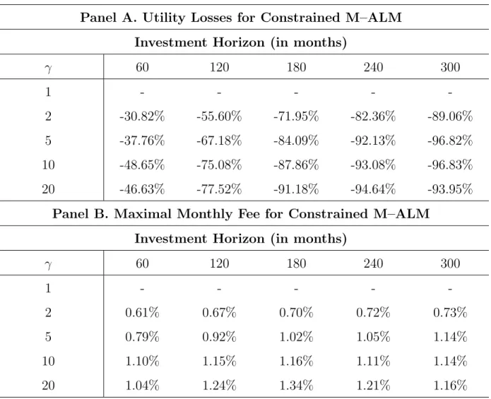
We report the results of this analysis in Table 4, considering an investor who faces short selling constraints. Panel A reports the utility losses of the M–ALM strategy over D–ALM. Panel B reports the largest monthly management fee an investor who now uses the M–ALM
would be prepared to pay to gain access to the D–ALM. JV highlight that fees re-scale the utility losses to facilitate comparisons across investment horizons.
As Panel A shows there are significant utility losses from not using the D–ALM. Utility losses increase as the horizon lengthens but conservative investors lose more than more risk tolerant investors. Our analysis suggests that a M-ALM investor with experiences utility losses that range from -37.76% (5-year investment horizon) to -96.82% (25-year investment horizon). The differences in the CE we document translate to management fees that range from 0.79% (5-year investment horizon) to 1.14% (25-year investment horizon) per month (Panel B). Additionally, the management fee increases significantly as investor risk tolerance falls. For a twenty five year investment horizon the maximum monthly management fee ranges from 0.73% (for a risk aversion of 2) to 1.16% (for a risk aversion of 20). The management fees for M–ALM investors who allow leverage in order to gain access to the D– ALM strategy range from 1.83% (5-year investment horizon) to 6.49% (25-year investment horizon) per month.
Our analysis to this point considers inflation–indexed bonds as possible investment assets. In what we present below we relax this assumption. Investing in inflation-indexed bonds might not be possible or desirable for a number of reasons. First, inflation indexed bonds are less liquid than nominal bonds (D’Amico et al., 2014; G¨urkaynak et al., 2010; Pflueger and Viceira, 2011). Second, despite the sharp growth of the linker market,10 a number of countries do not issue inflation-indexed bonds. Third, many investors might regard inflation indexed bonds unacceptable investments when the real yield to maturity is close to zero or even negative.11
We report the results of this analysis in Table 5, considering an investor who faces short selling constraints. Panel A reports the utility losses of the M–ALM strategy over the D– ALM strategy. Panel B reports the largest monthly management fee an investor who now uses the M–ALM would be prepared to pay to gain access to the D–ALM. We observe significant utility losses from not using the D–ALM strategy. A moderate risk averse M– ALM investor for example with experiences utility losses that range from -22.74% (5-year investment horizon) to -89.43% (25-year investment horizon). These losses translate to a maximal monthly management fees that range from 0.43% (5- year investment horizon) to 0.75% (25-year investment horizon) per month.
10Based on the Barclays Capital World Government Inflation-Linked Bond Index (WGILB) in April 2012, the global market value of inflation-indexed bonds was $2.0 trillion: US ($866 billion), UK ($549 billion), France ($235 billion), Italy ($132 billion).
The evidence in this Section overall suggests that the economic benefits of pursuing optimal portfolios with the D–ALM model are substantial. The outperformance over the M–ALM strategy is due to the implicit pursuance of tactical asset allocation within the strategic asset allocation framework. The D–ALM model exploits the predictability in the investment opportunity set while the M–ALM does not. This predictability has been shown to provide sizeable economic benefits even in instances when it is marginal.
6
Additional Analysis
In this section we study the effects of minimum and maximum funding constraints and alter-native liability benchmarks that include equities on asset allocation weights and utility for M–ALM and D–ALM investors. We also study the asset allocation and utility differences of a liability driven investor (dynamic ALM model) and an investor without liabilities (dynamic AM model, as in JV).
6.1
The economic value of dynamic rebalancing with funding ratio
constraints
The empirical evidence presented in the previous section shows substantial utility benefits if an investor with liabilities switches from M–ALM to D–ALM. The benefits are reduced but remain significant when the investor operates under short–selling constraints. Investing un-der short-selling constraints represents the typical investment framework in which individual investors invest. Defined benefit pension funds face, in addition to short-selling constraints, constraints with respect to the minimum funding ratio. In many countries regulations or internal pension fund rules dictate that when the funding ratio of the pension fund is close to, or below, a minimum threshold the sponsor of the pension fund is asked to increase contri-butions until it reaches the target value. There are also regulations and customary practices in many countries which “force” pension funds whose assets are much higher than liabilities to cease contribution until the surplus disappears (contribution holiday). In this Section we investigate the utility losses associated with the presence of funding ratio constraints.
Pugh (2006) provides a comprehensive review on the regulations of the pension funds in the OECD countries. Minimum fund requirements whether imposed by legislation or not aim to protect plan member benefits. For example, for Dutch pension funds the minimum funding level is set at 105%, while the maximum (or target) funding ratio is on average 130%.
For UK pension plans there is no minimum funding level imposed by regulation but each pension fund is required to adopt a statutory funding objective. In the UK pension funds face a maximum funding level constrain which dictates that pension fund assets should not exceed 105% of accrued liabilities.
The imposition of minimum and maximum funding level constraints means that outcomes below the minimum funding level and above the maximum funding level are not possible. In our analysis we assume that the fund sponsor increases immediately contributions when the asset liability ratio reaches the minimum fund level.12Similarly when the asset to liability ra-tio reaches the maximum funding level we assume that the fund sponsor ceases contribura-tions until the funding ratio falls below the maximum funding level. In the simulations we pursue to address these issues we assume (a) that the asset liability ratio should not fall below 1 and (b) that the target minimum funding level is 90% (asset/liability ratio of 90%). In both cases that contributions cease when the asset to liability ratio reaches 135%. We recognize that the nature of our model does not allow to internalize the funding ratio constraint in the optimal solution as in approaches that involve numerical analysis (see, e.g. Berkelaar and Kouwenberg(2010)).
The effect of minimum–maximum funding ratios on the distribution of funding ratios is significant. The median funding ratio for the M–ALM strategy increases from 97% in the five–year horizon to a modest 113% at the end of twenty five years. Increasing the minimum funding ratio from 90% to 100% and keeping the same maximum funding ratio (135%) leads as expected to better future funding ratios. The median funding ratio increases from 102% in the five-year horizon to 108% at the end of twenty five years (see Table B1, Panels B and C, Appendix). Imposing a min–max funding ratio constraint of 90%-135% reduces considerably the median funding ratios for the D-ALM investor too. At the end of twenty five years the median funding ratio is 129%. Similarly if the minimum funding ratio is 100% the median funding ratio at the twenty five year horizon is slightly higher at 130% (see Table B2, Panels B and C, Appendix).
In relative terms, the M–ALM strategy suffers from lower minimum funding ratios. For instance, the minimum funding ratio for the M–ALM strategy is 0.01 at the twenty five year horizon, while the minimum funding ratio for the D–ALM strategy is 0.91 over the same horizon. Moreover, in the absence of funding ratio constraints the median/mean funding ratio of the D–ALM strategy is always higher than the median/mean funding ratio of the
12In practice the pension fund with the sponsor and the advice of the pension fund’s actuary agree a multi– year plan of increased contributions or a contribution holiday until the deficit or surplus are eliminated.
M–ALM strategy, across all investment horizons. The latter are consistent with the results we present earlier, i.e. that the D–ALM strategy exhibits utility benefits over the M–ALM for a constrained investor in the absence of regulatory constraints. Imposing a min-max funding ratio constrain of 90% (100%) -135% reduces considerably the difference of the median/mean funding ratios between the two strategies.
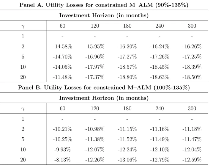
To investigate the economic value of the D–ALM strategy in the presence of funding ratio constraints we calculate the utility loss from using the M–ALM (instead of the D–ALM) strategy as well as the associated management fee with results reported in Table 6 and Table 7 respectively. For example, a M–ALM investor with γ = 5 experiences utility losses that range between -14.70% (5-year investment horizon) and -17.25% (25-year investment horizon) for a min-max funding ratio constraint of 90% -135%. The utility losses are lower when the asset liability ratio is required to stay in the 100% - 135% range. Similarly, from the results reported in Table7we show that the largest monthly management fee an investor who currently uses the M–ALM would pay to gain access to the D–ALM ranges from 0.25% (5-year horizon) to to 0.06% (25-year horizon).
Collectively, the evidence in this Section suggests that imposing tight funding constraints reduces but does not eliminate the benefits from hedging dynamically the investment oppor-tunity set and liabilities.
6.2
Asset Liability Management vs. Asset Management: Asset
Allocation and Utility Implications
In this Section we examine the structure of the optimal portfolios and the utility implications of the proposed ALM model compared with the AM model developed by JV. The data inputs are the same as those described in section 4.
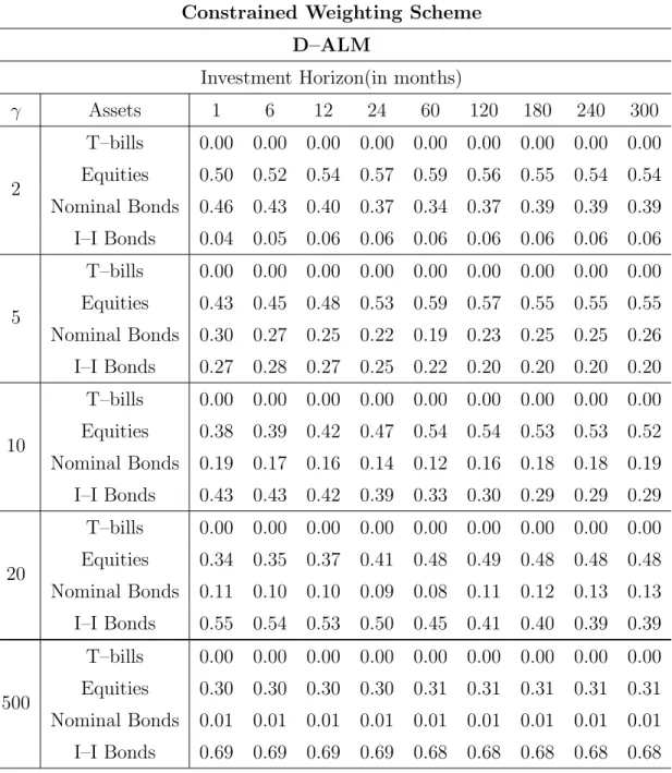
Table 8 reports the asset allocation at any investment horizon ranging from 1 to 300 months (25 years) and risk-aversion levels ranging from 2 to 500 (γ = 2,5,10,20,500) for both the dynamic ALM and AM models. Panel A of Table 8 tabulates the allocations for portfolios with no constraints on portfolio weights. Panel B in Table 8 presents the optimal weights assuming borrowing is not allowed. The 1–month mean percentage portfolio allocation corresponds to the one–period (myopic) asset allocation.
We begin our discussion with the case of unconstrained portfolio weights. For low and moderate levels of risk-aversion equity allocations are similar for both AM and ALM models. Equity allocations increase as the investment horizon increases and decrease as risk aversion increases. The allocation to equities when γ = 5 for example ranges from 0.56 (0.56) in 6
months to 1.61 (1.62) in 300 months for an ALM (AM) investor.
We observe significant differences in the allocations to inflation–indexed bonds. These differences are almost entirely attributable to the myopic portfolio. The myopic allocation to real bonds for an investor with for example is 73% and only increases to 89% for the same investor with a twenty five year investment horizon. On the other hand, the allocation to real bonds for the AM investor who ignores liabilities is very low (even negative) both across different levels of risk-aversion and investment horizons. For an ALM investor the allocation to inflation indexed bonds is increasing in the degree of risk aversion.Brennan and Xia(2002) also find that optimal real terminal wealth portfolios are tilted towards inflation–indexed bonds as risk–aversion increases, and are entirely invested in inflation–indexed bonds in the limit.
AM and ALM investors allocate similar amounts to nominal bonds for low levels of risk aversion and moderate levels up to five-year investment horizon, but the differences become material for relatively high risk aversion levels. ALM optimal portfolios comprise lower allocations to nominal bonds than AM optimal portfolios. The lower allocation to nominal bonds in the ALM optimal portfolios seems to come “at the expense” of higher allocation to inflation-indexed bonds relative to AM optimal portfolios. The increasing allocation to inflation indexed bonds reflects the myopic and intertemporal hedging demand for inflation-indexed bonds by an ALM investor to hedge real liabilities.
The allocation to T–bills is negative regardless of the length of the investment horizon and the level of risk aversion in ALM optimal portfolios; T–bills are a bad liability hedge asset class since their correlation with liabilities is negative at all investment horizons. On the other hand, AM optimal portfolios with moderate and high levels of risk aversion are heavily invested in T–bills, especially at short horizons.
Assuming for short–selling constraints, both dynamic ALM and AM investors increase their allocation to stocks as the investment horizon increases. ALM optimal portfolios com-prise lower allocations to equities than AM optimal portfolios for moderate and high levels of risk aversion. For example dynamic ALM (AM) investors with risk aversion equal to 5 increase the equity weights from 28% (45%) when the investment horizon is one month to 48% (56%) when the horizon is 300 months.
AM investors with moderate risk aversion (γ = 5) allocate 45% in nominal bonds in the short term and the allocation decreases to 39% for long term investors. ALM investors start with 29% at the monthly horizon and invest 25% at the 300 month horizon. The asset allocation to real bonds for AM investors is almost negligible at all investment horizons and
levels of risk aversion. For ALM investors is slightly over 40% and remains constant over the horizon.
Our analysis so far finds that the composition of the optimal portfolios that we obtain when we use the proposed model is different from the composition of the optimal portfolios obtained through the model in JV. Hence, we need to investigate the utility implications that are associated with these differences. Our analysis utilizes the certainty equivalent of the funding ratio, as defined in section5. For the AM strategy (JV), we compute the optimal allocation policy, the realized terminal funding ratio, and the realized utility of the terminal funding ratio along each path. We therefore consider that the AM investor has the same liabilities as the ALM investor.
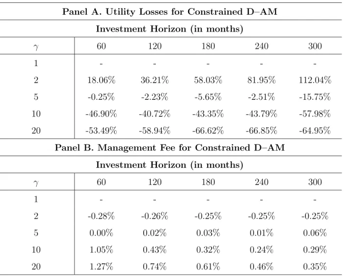
Table 9reports the utility losses of the D–AM strategy over D–ALM (Panel A) and the largest monthly management fee an investor who now uses the D–AM would be prepared to pay to gain access to the D–ALM (Panel B). We consider an investor who faces short selling constraints. The utility loses for investor with γ = 5 who allocates her wealth according to JV, range from -0.25% (1–month investment horizon) to -15.75% (300–months investment horizon). Accounting for liabilities, under short-sale constraints, makes little difference to the asset allocation and utility of AM and ALM investors with low to moderate risk aversion (γ <5). For pension funds with young membership and few retired members, liabilities do not play an important role in their asset allocation decision. For more risk averse investors (γ >5) liabilities play a very important role in the determination of the optimal asset mix. At an investment horizon of 300 months for example, the utility losses from disregarding liabilities range from -15.75% (γ = 5) to -64.95% (γ = 20). The differences in CE overall translate to management fees that range between 0.06% and 0.35% per month or between 0.72% and 4.20% per annum, respectively.
Collectively, we observe material differences between optimal ALM and optimal AM port-folios in inflation–indexed bonds and T–Bills (for all investors), and in equities and nominal bonds (for moderate to highly risk-averse investors). HMSS find also significant differences in the portfolio allocations of myopic asset-liability investors who ignore liabilities. Further-more, the economic benefits of pursuing optimal portfolios with our model are significant for moderate and highly risk averse investors. The economic benefits over the JV strategy arise from the intertemporal liability hedging portfolio. This portfolio is a unique element of our model. As we highlight earlier, it takes into account the correlation between the innovations of liabilities and the innovations in the changes of the state variables.
6.3
Alternative Liability Benchmark
The asset allocation of investors with liabilities depends critically on the properties of the investor’s liabilities. In our model liabilities are exogenously determined following the ap-proach of other papers in the academic literature (Hoevenaars et al., 2008; Amenc et al., 2009;Binsbergen and Brandt,2014). In practice a pension fund’s liabilities will be a function of many parameters defined in the pension fund rules. Partial or full indexation of pensions in payment and the particular mix of active, deferred and retired members are two of the most important characteristics of a pension’s liabilities.
Index–linked bonds will be the appropriate benchmark for a pension fund’s fully indexed Accumulated Benefit Obligations (ABO). It will also be a good proxy for a mature pension fund’s Projected Benefit Obligations (PBO). For defined benefit plans PBO liabilities will depend on economic productivity. To hedge part of PBO liabilities Black (1989), Lucas and Zeldes (2006;2009), Waring(2011) among others suggest that equities might provide a better hedge assuming that wage growth and equities are positively correlated.13
For mature pension funds with full or partial indexation of pensions in payment a portfolio of index–linked bonds and equities would be a more appropriate liability benchmark. The exact mix of equities and index-linked bonds will depend on the particular characteristics of the pension fund but a 30% equity, 70% index–linked bonds portfolio represents a reasonable benchmark for a mature pension fund where wage growth does not affect the pensions of retired employees.
Table 10 shows the asset allocation of a dynamic and myopic investor with liabilities, proxied by a portfolio of 30% equities and 70% index–linked bonds, assuming short sales are not allowed. When equities are part of the liability benchmark the investor as expected allocates more to equities, at the expense of index-linked bonds compared with an investor whose liabilities are exclusively index–linked bonds. Both dynamic and myopic investors in-vest sizeable part of their portfolio in equities. The percentage allocated to equities decreases from over 50% for low risk aversion dynamic investors to 30% for very conservative investors. For myopic, low risk aversion, long-term investors the percentage invested in equities is close to 80%. For moderate risk aversion (γ = 5,10 ) the weight invested in equities is between 42% (γ = 5 , horizon 1 month) to 52% (γ = 10 , horizon 300 months). Investors with 100% index-linked liabilities invest less in equities and more in index-linked bonds except when
13Empirical evidence on the relation between wages and equities are controversial. Benzoni et al.(2007) find that wages and equities are highly correlated over long horizons.Lustig and Van Nieuwerburgh(2008) report a negative relation.
risk aversion is low and therefore liabilities are not important in the asset allocation decision. The percentage allocated to nominal bonds is very similar under both liability benchmarks. In unreported results, we find that the new liability benchmark does not change significantly the utility gains of the D–ALM over the M–ALM strategy.
Excluding inflation-linked bonds from the investor’s investment opportunity set reduces marginally the weight of equities but the main effect is a substitution of inflation-linked bonds with nominal bonds. An investor with average risk aversion (γ = 5 ) invests over 50% of her portfolio in nominal bonds (detailed allocation results available from the authors upon request).
7
Conclusions
In this paper we develop a closed-form solution for the dynamic multi–period portfolio choice problem in the presence of liabilities. The model is analytically tractable allowing the study and interpretation of factors affecting optimal portfolio choice in an ALM framework. The model can accommodate investment opportunity sets which comprise any number of assets and state variables. It also allows for time–varying risk premia and interest rates.
Investors who invest their portfolios with the objective to meet future liabilities, tak-ing time–varytak-ing opportunities into account results in different portfolios compared with investors who do not. Access to a dynamic asset liability model provides significant utility benefits to a myopic investor. The benefits are reduced but not eliminated when the in-vestor faces short-sell constraints and in particular the ability to borrow. The model should be of particular interest to individual investors with liabilities who invest under short–sell constraints.
Under pension fund regulation and internal rules, pension funds usually operate within funding ratio constraints. Pension fund strategic asset allocation in practice tend to follow a myopic asset allocation strategy that is re-visited every three to five years and usually ignores time–varying opportunities. Imposing funding ratio constraints reduces but do not elimi-nate the benefits of exploiting return predictability and hedging dynamically the investment opportunity set and liabilities.
We believe that there are several promising directions for future research. While we as-sume that our investor is endowed with a power utility of real end-of-period funding ratio for a finite horizon, it would be valuable to consider an ALM investor who takes into ac-count intermediate consumption or labor income (Campbell et al.,2003;Rapach and Wohar,
2009). Another extension would be to investigate the optimal asset allocation and the utility implications of a dynamic investor who faces different types of liabilities and longevity and demographic risks.