Self-Imitation Regularization: Regularizing Neural Networks by Leveraging Their Dark Knowledge

Image: Dark Matter in a Simulated Universe; Illustration Credit & Copyright: Tom Abel & Ralf Kaehler (KIPAC, SLAC), AMNH; Published on APOD (https://apod.nasa.gov/apod/ap171031.html, as of February 4, 2019).

Rights of use obtained from the copyright holder, Tom Abel (on May 9, 2019). Special thanks for that.

Self-Imitation Regularization:

Regularizing Neural Networks by

Leveraging Their Dark Knowledge

Self-Imitation Regularization:

Regularisierung Neuronaler Netze durch Verwendung ihres Dark Knowledges Bachelor-Thesis von Jonas Jäger aus Mannheim

Juni 2019

Fachbereich Informatik Knowledge Engineering Group

Self-Imitation Regularization:

Regularizing Neural Networks by Leveraging Their Dark Knowledge Self-Imitation Regularization:

Regularisierung Neuronaler Netze durch Verwendung ihres Dark Knowledges Vorgelegte Bachelor-Thesis von Jonas Jäger aus Mannheim

1. Gutachten: Prof. Dr. Johannes Fürnkranz 2. Gutachten: Dr. Eneldo Loza Mencía Tag der Einreichung:

Bitte zitieren Sie dieses Dokument als: Please cite this document as:

URN: urn:nbn:de:tuda-tuprints-87175

URL: http://tuprints.ulb.tu-darmstadt.de/8717 Dieses Dokument wird bereitgestellt von tuprints, E-Publishing-Service der TU Darmstadt

This document is provided by tuprints, E-Publishing-Service of the TU Darmstadt http://tuprints.ulb.tu-darmstadt.de

[email protected]

Die Veröffentlichung steht unter folgender Creative Commons Lizenz: This publication is licensed under the following Creative Commons license:

Namensnennung – Keine kommerzielle Nutzung – Keine Bearbeitung 4.0 Deutschland Attribution – Non-commercial – No Derivatives 4.0 Germany

The universe is made mostly of dark matter and dark energy, and we don’t know what either of them is.

Saul Perlmutter, 2011 Nobel laureate in Physics

Physicists will tell you that 95% of the stuffin the universe is not what they were paying attention to – it is something else.

[. . . ] The point of [dark knowledge] that I want to show you [is] that 95% of what a neural network learns is not what you are trying to get it to learn and is not what you test it on

– it is something else.a

Geoffrey Hinton, 2018 Turing recipient for his research on artificial neural networks

a _{He began his talk with these words, in the Excellent Lecture Series at TTIC (Toyota Technological Institute at} Chicago) given on October 2, 2014.http://www.ttic.edu/dls-2014-2015/(as of January 9, 2019)

Abstract

Deep Learning, the learning of deep neural networks, is nowadays indispensable not only in the fields of computer science and information technology but also in innumerable areas of daily life. It is one of the key technologies in the development of artificial intelligence and will continue to be of great importance in the future, e.g., in the development of autonomous driving. Since the data for learning such (deep) neural networks is clearly limited and therefore the neural network cannot be prepared for all possible data which have to be handled in real-life situations, a solid generalization capability is necessary. This means the ability to acquire a general concept from the training data, so that the task associated with the data is properly understood and the training data is not simply memorized. An essential component behind such a generalization capability is regularization.

A regularization procedure causes a neural network to generalize (better) when learning from data. Various, commonly and widespread used regularization procedures exist, which, for example, limit the weights in the neural network (parameters by whose adaptation learning takes place) or temporarily change its structure, and thus implicitly aim for the neural network to make better predictions on as yet unseen data.

Self-Imitation Regularization (SIR) is presented in this thesis and is an easy to implement regular-ization procedure which, in contrast to the established standard regularregular-ization procedures, explic-itly addresses the actual objective – the formation of predictions – and only implicexplic-itly influences the weights/parameters in the neural network. The existing (dark) knowledge of the learning neural net-work is used and explicitly involved in the learning principles (i.e., the error function to be minimized) of the neural network. Since this is one’s own knowledge, which, in turn, is made available during learning, this can be seen as a form of self-imitation. For a given data example, the (dark) knowledge contains, on the one hand, information about the similarities to other classes (in a classification problem, a neu-ral network predicts classes and classifies the data). On the other hand, it quantifies (relative to other data examples) the confidence of the neural network in the prediction for this data example. Intuitively, through self-imitation, this information induces a questioning behavior regarding the correctness of the given solutions in the training data as well as deepens the understanding of correlations and similarities between the classes.

Besides the regularization ability, which has strong guarantees of success (partially under statistical significance), the use of SIR stabilizes the training, increases the data efficiency and is resistant to er-roneous data labels, which was demonstrated in various experiments. It is also applicable to very deep neural network architectures and can be combined with some standard regularization methods (i.e., dropout and maxnorm regularization). The implementation and additional computation effort is very low while the hyperparameter tuning is simple.

In this thesis, experimental results on the use of SIR are analyzed and evaluated using several pro-cedures, and the learned neural networks are examined closely in order to explain the regularization behavior along with accompanying properties.

Zusammenfassung

Deep Learning, das Lernen von tiefen Neuronalen Netzen, ist heutzutage nicht nur aus der Informatik und Informationstechnologie, sondern auch aus unzähligen Bereichen des Alltags nicht mehr wegzuden-ken. Es bildet eine der Schlüsseltechnologien in der Entwicklung von Künstlicher Intelligenz und wird auch für die Zukunft von großer Bedeutung sein, wie bspw. in der Entwicklung des Autonomen Fahrens. Da die Daten zum Lernen von solchen (tiefen) Neuronalen Netzen natürlich begrenzt sind und dieses somit nicht auf sämtliche mögliche Daten, die im späteren realen Einsatz verarbeiten werden müssen, vorbereitet werden kann, ist eine solide Generalisierungsfähigkeit notwendig. Also die Fähigkeit ein ge-nerelles Konzept aus den Lerndaten zu lernen, damit die mit den Daten verbundene Aufgabe wirklich verstanden wird und die präsentierten Daten nicht einfach nur auswendig gelernt werden. Hinter einer solchen Generalisierungsfähigkeit steckt eine wesentliche Technik: Regularisierung.

Ein Regularisierungsverfahren bewirkt das (bessere) Generalisieren eines Neuronalen Netzes beim Lernen aus Daten. Diverse, viel eingesetzte und weit verbreitete Regularisierungsverfahren existieren, die bspw. die Gewichte im Neuronalen Netz beschränken (Parameter durch deren Anpassung das Lernen stattfindet) oder dessen Struktur temporär verändern und damit implizit bezweckt werden soll, dass das Neuronale Netz bessere Vorhersagen auf ungesehenen Daten trifft.

Self-Imitation Regularization (SIR) wird in dieser Thesis vorgestellt und ist ein einfach zu implemen-tierendes Regularisierungsverfahren, das im Gegensatz zu den etablierten Standardregularisierungsver-fahren explizit am eigentlichen Ziel – der Formung der Vorhersagen – ansetzt und nur implizit die Ge-wichte/Parameter im Neuronalen Netz beeinflusst. Dabei wird das vorhandene (Dark) Knowledge des lernenden Neuronalen Netzes genutzt und explizit in die Lernprinzipien (d.h. die Fehlerfunktion, die minimiert werden soll) des Neuronalen Netzes involviert. Da es sich um das eigene Wissen handelt, was nun wiederum beim Lernen zusätzlich zur Verfügung gestellt wird, kann dies als eine Form von Selbstimitation gesehen werden. Das (Dark) Knowledge beinhaltet für ein gegebenes Datenbeispiel zum einen Informationen über die Ähnlichkeiten zu anderen Klassen (in einem Klassifizierungsproblem sagt ein Neuronales Netz Klassen vorher, um damit die Daten zu klassifizieren). Zum anderen quantifiziert dies (relativ zu anderen Datenbeispielen) darüber, wie sicher sich das Neuronale Netz beim Treffen der Vorhersage zu diesem Datenbeispiel ist. Intuitiv gesehen wird durch diese Informationen mittels der Selbst-Imitation sowohl ein hinterfragendes Verhalten bzgl. der Korrektheit der vorgegebenen Lösun-gen in den Lerndaten hervorgerufen, als auch das Verständnis über Zusammenhänge und Ähnlichkeiten zwischen den Klassen vertieft.

Neben der eigentlichen Regularisierungsfähigkeit, die starke Erfolgsgarantien (teilweise mit statisti-scher Signifikanz) aufweist, stabilisiert der Einsatz von SIR das Training, erhöht die Dateneffizienz und erweist sich als resistent gegen fehlerhafte Datenlabel, was in diversen Experimenten gezeigt werden konnte. Auch ist es auf sehr tiefen Netzarchitekturen anwendbar und kann mit manchen Standard-regularisierungsmethoden (Dropout und Maxnorm) kombiniert werden. Der Implementierungs- sowie zusätzliche Berechnungsaufwand ist sehr gering und das Tunen der Hyperparameter ist einfach.

In der Thesis werden experimentelle Ergebnisse zum Einsatz von SIR mit verschiedenen Verfahren ausgewertet und evaluiert, sowie die gelernten Neuronalen Netze genauer untersucht, um das Regulari-sierungsverhalten samt einhergehender Eigenschaften zu erklären.

Contents

2.1.1. Categories of Machine Learning . . . 19

2.1.2. Algorithms in Machine Learning . . . 23

2.1.3. Expressive power and separability . . . 24

2.1.4. Generalization . . . 25

2.2. Artificial Neural Networks . . . 26

2.2.1. The neuron . . . 28

2.2.2. Layer of neurons . . . 29

2.2.3. Multi-Layer Perceptron (MLP); or, stacking layers of neurons . . . 31

2.2.4. Gradient-based learning . . . 33

2.3. Convolutional Neural Networks (CNNs) . . . 37

2.3.1. Convolutional layer . . . 38

2.3.2. Pooling layer . . . 39

2.4. Activation functions . . . 40

2.4.1. Sigmoidal activation functions . . . 41

2.4.2. Rectifier activation function variants . . . 41

2.5. Loss functions . . . 43

2.5.1. Mean squared error . . . 44

2.5.2. Cross entropy loss . . . 44

2.6. Softmax . . . 47

2.6.1. Temperature Softmax . . . 51

2.6.2. Combination of softmax and cross entropy loss . . . 52

2.7. Regularization . . . 53

2.7.1. Parameter norm penalty regularization . . . 54

2.7.2. Maxnorm constraint . . . 55

2.7.3. Dropout . . . 56

2.8. Knowledge Distillation and Dark Knowledge . . . 57

3. Self-Imitation Regularization (SIR) 61 3.1. Hypotheses . . . 64 7

3.2. Further variants of Self-Imitation Regularization (SIR) . . . 67

3.2.1. Penalty formulation . . . 67

3.2.2. Target network . . . 69

3.3. Preliminary studies in Knowledge Distillation (KD) . . . 70

3.3.1. Comparison: temperature and the chained softmax function . . . 70

3.3.2. Comparison: Symmetric and asymmetric imitation . . . 71

4. Experiments 73 4.1. Experimental set-ups . . . 73

4.1.1. Noisy data labels . . . 73

4.1.2. Learning on a small training data subset . . . 73

4.1.3. Reduced training samples of a class . . . 74

4.1.4. Standard regularization methods . . . 74

4.2. Data sets . . . 74

4.3. Neural network architectures . . . 77

4.4. Evaluation methodologies . . . 79

4.4.1. Metrics . . . 79

4.4.2. Statistical tests . . . 83

5. Experimental results 87 5.1. Regularization capability . . . 87

5.1.1. Regularization ability with other regularizers being present . . . 91

5.1.2. Overfitting in the later training course . . . 93

5.2. On the functioning of Self-Imitation Regularization (SIR) . . . 94

5.2.1. Predictions and soft targets investigation . . . 94

5.2.2. Parameters investigation . . . 98

5.2.3. (Ranking) quality of the soft targets/predictions . . . 101

5.3. Noisy data label compensation . . . 104

5.3.1. Robust learning despite noisy labels . . . 104

5.3.2. Correcting ability of noisy training labels . . . 110

5.4. Learning from other classes . . . 113

5.5. Training stabilization . . . 115

5.6. Depth of a neural network . . . 116

5.7. Pre-fitting . . . 119

6. Conclusion 121 6.1. Future work . . . 124

6.1.1. Further investigations . . . 125

6.1.2. Extensions and improvements of Self-Imitation Regularization (SIR) . . . 126

Acknowledgments 129

A. Experimental results 139

A.1. Statistical tests raw performance scores . . . 139 A.1.1. Testing Self-Imitation regularized against unregularized neural networks . . . 139 A.1.2. Testing neural networks with SIR combined with a standard regularizer against

this standard regularizer on its own . . . 141 A.2. Noisy data labels results . . . 145

List of Figures

2.1. Separability in classification problems . . . 24

2.2. Generalization behavior in learning curves . . . 25

2.3. Artificial neuron: a schematic visualization . . . 30

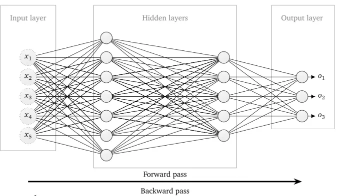
2.4. Artificial neural network or Multi-Layer Perceptron (MLP): a schematic visualization . . . 31

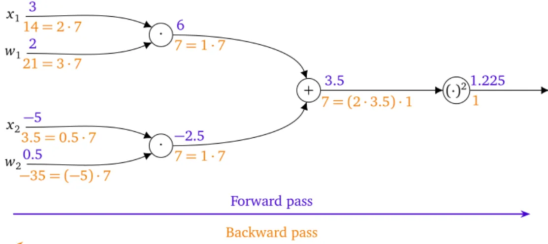
2.5. Exemplary application of the backpropagation algorithm on a computational graph . . . . 36

2.6. Exemplary visualization of the convolution operation . . . 38

2.7. Exemplary visualization of max pooling . . . 39

2.8. Activation functions . . . 40

2.9. Plot of the negative log probability mappingp_7! log₍p₎ . . . 45

2.10.Softmax function mapping properties . . . 48

2.11.Temperature softmax function mapping properties (on different temperatures) . . . 52

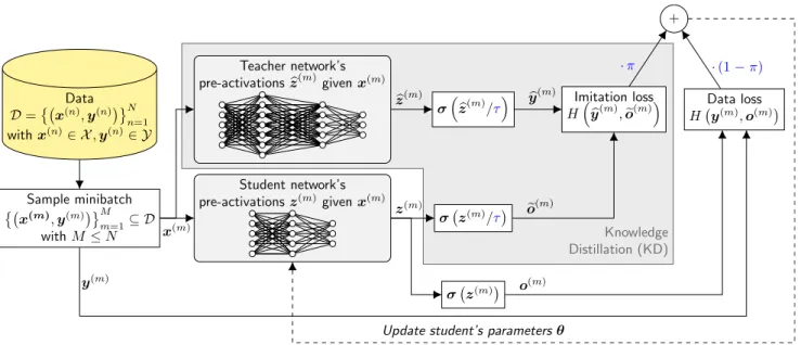
2.12.Knowledge Distillation (KD) framework diagram . . . 59

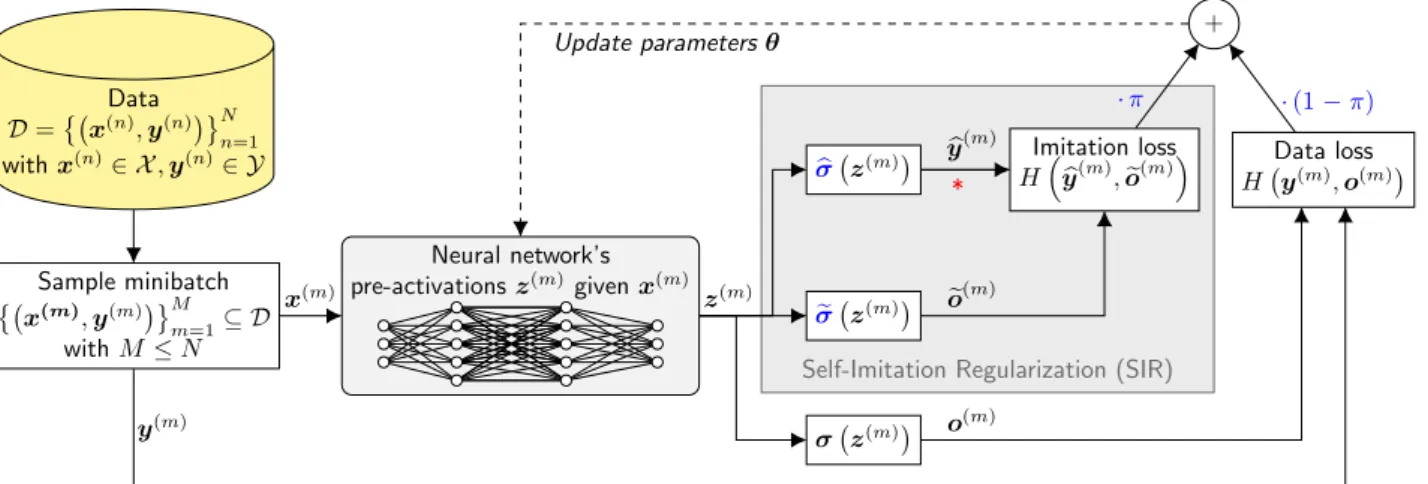
3.1. Self-Imitation Regularization (SIR) framework diagram . . . 62

3.2. ⇣-chain softmax function mapping properties (on different values for⇣) . . . 63

3.3. Preliminary KD experiments: comparison between temperature and chained softmax func-tion . . . 71

4.1. Exemplary samples from the (visual) training data sets . . . 78

5.1. Differences in test accuracy on multiple data sets between self-imitation regularized neural networks compared to unregularized ones . . . 89

5.2. Mean test accuracy of different SIR settings on multiple data sets plotted over the imitation rate⇡ . . . 90

5.3. Learning curves on the CIFAR-10 data set and differently regularized neural networks . . . 93

5.4. Best test accuracy achieved while learning compared to the final test accuracy . . . 94

5.5. Mean normalized entropy of (prediction) distributions from learned neural networks . . . 95

5.6. Exemplary prediction distributions of two learned neural networks (SIR vs. unregularized) 97 5.7. Mean lengths (L1_{-norm and L}2_{-norm) of parameter vectors . . . 99}

5.8. Average softmax distributions per class in heat maps on the CIFAR-10 test data set . . . 101

5.9. Test accuracy plotted over different amounts of label noise . . . 104

5.10.Confusion matrices on the CIFAR-10 test data set after training with 50% label noise . . . 105

5.11.Mean test accuracy (to different degrees of label noise) plotted over the imitation rate⇡ . 106 5.12.Best test accuracy achieved while learning on different amounts of label noise . . . 107

5.13.Mean test accuracy plotted to different degrees of label noise in comparison with standard regularization methods . . . 108

5.14.Peak test accuracy plotted to different degrees of label noise in combination with standard regularization methods . . . 109

5.15.Correction ability of the noisified training data samples (in accuracy) . . . 110

5.16.Correction ability of the noisified training data samples (in position error) . . . 111 11

5.17.Incorrect label uncertainty factors on training data with label noise . . . 112 5.18.Performance for classdogwhose samples had been reduced in the training set to different

degrees . . . 114 5.19.SIR on the CIFAR-10 data set with theResNetarchitecture at different depths . . . 117 5.20.SIR on the CIFAR-10 data set (with label noise) with theResNetarchitecture at different

List of Tables

3.1. Preliminary KD experiments: comparison between symmetric and asymmetric imitation . 72 4.1. Information about the data sets . . . 75 4.2. Information about the experimental neural network architectures . . . 77 5.1. Results from the statistical tests for different experimental configurations over multiple

data sets comparing the performance of self-imitation regularized neural networks to un-regularized ones . . . 88 5.2. Further statistical tests with a different SIR hyperparameter setting for different

experi-mental configurations over multiple data sets comparing the performance of self-imitation regularized neural networks to unregularized ones . . . 90 5.3. Results from the statistical tests for different experimental configurations over multiple

data sets comparing the performance of neural networks with SIR and a standard regu-larizer to a neural network regularized solely with this standard reguregu-larizer . . . 92 5.4. Evaluation metrics regarding the ranking quality of soft predictions . . . 103 A.1. Performance scores and pair-wise differences used for statistical testing (SIR with target

gradients) . . . 139 A.2. Performance scores and pair-wise differences used for statistical testing (SIR without

tar-get gradients) . . . 140 A.3. Performance scores and pair-wise differences used for statistical testing comparing SIR

combined withL1_{-norm reg. to solely L}1_{-norm reg. (SIR with target gradients) . . . 141}

A.4. Performance scores and pair-wise differences used for statistical testing comparing SIR combined withL2_{-norm reg. to solely L}2_{-norm reg. (SIR with target gradients) . . . 141}

A.5. Performance scores and pair-wise differences used for statistical testing comparing SIR combined with maxnorm to solely maxnorm (SIR with target gradients) . . . 142 A.6. Performance scores and pair-wise differences used for statistical testing comparing SIR

combined with dropout to solely dropout (SIR with target gradients) . . . 142 A.7. Performance scores and pair-wise differences used for statistical testing comparing SIR

combined withL1_{-norm reg. to solely L}1_{-norm reg. (SIR without target gradients) . . . 143}

A.8. Performance scores and pair-wise differences used for statistical testing comparing SIR combined withL2_{-norm reg. to solely L}2_{-norm reg. (SIR without target gradients) . . . 143}

A.9. Performance scores and pair-wise differences used for statistical testing comparing SIR combined with maxnorm to solely maxnorm (SIR without target gradients) . . . 144 A.10.Performance scores and pair-wise differences used for statistical testing comparing SIR

combined with dropout to solely dropout (SIR without target gradients) . . . 144 A.11.Label noise performance scores . . . 145 A.12.Label noise performance scores . . . 146

Notation

Math notation:

The math notation does mainly follow the notation used in Petersen et al. (2004) and Goodfellow et al. (2016).

A Matrix

Ai Matrix indexed for some purpose A(i) _{Matrix indexed for some purpose} A> _{Transpose of matrixA}

I Identity matrix (i.e., ones on the diagonal and zeros elsewhere)

a Vector

a_i Vector indexed for some purpose

a(i) _{Vector indexed for some purpose} a> _{Transpose of vectora}

1 All-ones vector (i.e., every element is equal to one)

ka_ka a-norm of vectora

a Scalar

a(i) _{Scalar indexed for some purpose}

ai j The element in theith row and jth column of the matrixA

ai,j The element in theith row and jth column of the matrixA

ai Theith element of vector a(or taken from a set)

f_i(a₎ Theith element of the output vector of the function f, i.e., equal to y_i for y = f(a)

A Set

N Natural numbers

R Real numbers

R+ _{Positive real numbers (exclude zero)} Rn _{n-dimensional (real valued) vector space} P(A₎ Power set of setA

P(X a) Probability that random variableX is greater than or equal toa E

X⇠p(·){·} Expected value of{·}for the random variableX distributed according top(·)

fL _{Function f labeled for some purpose}

f g(·) The composition of functions f and g, i.e., f(g(·)) raf(·) Gradient of function f with respect to to vectora

@f(·)

@a or @@af(·) Partial derivative of function f with respect to scalara expa Exponential function ofa, i.e.,ea

loga The natural logarithm ofa, i.e., equal tolnaorlog_ea

Abbreviations:

ANN Artificial Neural Network

CNN Convolutional Neural Network

KD Knowledge Distillation

ML Machine Learning

MLP Multi-Layer Perceptron

MSE mean squared error

NN Neural Network

RL Reinforcement Learning

RNN Recurrent Neural Network

1 Introduction

When Geoffrey Hinton, Oriol Vinyals, and Jeff Dean introduced a method they called "Knowledge dis-tillation" in 2014 (Hinton et al., 2015), they shed light upon an intriguing property of artificial neural networks that they referred to as dark knowledge; or at least Geoffrey Hinton did so in a talk named "Dark knowledge" in the Excellent Lecture Series at Toyota Technological Institute at Chicago (TTIC) given on October 2, 2014.

Clearly, this term is more metaphoric than scientific but gives a vivid description of the subject. As quoted on the opening pages, the term dark knowledge is derived from the phenomena of dark matter and dark energy (Abbott et al., 2016) used in astrophysics and yields a description for the material that the universe is mostly made of. To be more precise, dark matter makes up 27% and dark energy 68% of the universe which results in the impressive total portion of 95%. Although the effects and necessity of the existence of dark matter and dark energy were already demonstrated in the 20th century as the reasons why rotating galaxies do not fly apart and the universe is permanently expanding, respectively. However, it is astounding that it is entirely unknown what dark matter and dark energy is made of. Therefore, it seems that over the past decades, most of the research that has been highly successful in physics has been based on areas dealing with the remaining 5% of ordinary matter. The visualization of a dark matter simulation on the title page of this thesis vividly shows a possible segmentation of the universe into complex filaments of dark matter (in black) and rare clusters of ordinary matter (orangeish glowing), and demonstrates how small the ordinary matter share of 5% is.

Returning to computer science, machine learning, and the explanation of Geoffrey Hinton’s dark knowledge term in artificial neural networks: In addition to learning the ability to make an accurate prediction based on a prediction task, such as a classification problem – which is a typical setting artifi-cial neural networks are deployed in – artifiartifi-cial neural networks generally acquire much more knowledge as a side product of generalization during the course of learning. For example, in this additional knowl-edge lies the understanding of similarity and correlation between the different outcomes to be predicted (i.e., the different classes in a classification setting). However, since in most cases of application the final prediction is of interest only, the research community has mainly paid attention to only a small part of knowledge an artificial neural network acquires which is measured by the final prediction performance. Again, note that the given information in the presented quote expound dark knowledge as an analogy of dark matter and dark energy serves more motivational purposes than scientific significance. Especially the percentage of 95% is not related to any portion of knowledge within an artificial neural network in general. However, this dark knowledge phenomenon is clarified in Hinton et al. (2015) explaining the method of knowledge distillation as a concrete procedure of training artificial neural networks, which is going to be explained in more detail in Sec. 2.8. Roughly, knowledge distillation can be described as a technique that allows distilling the (dark) knowledge in a large and deep neural network into another much smaller neural network, which would not be able to acquire that knowledge from the data on its own. These ideas and concepts were taken up to develop a novel regularization method, which is introduced in this thesis.

Regularization encompasses all the techniques supporting a neural network learning the general con-cept from the data better and to prevent the neural network from overfitting on the (training) data. Overfitting describes the memorization of idiosyncrasies in this data or even of all data examples. If 17

overfitting cannot be prevented and such generalization cannot be achieved (e.g., by missing or using unsuitable regularization methods), this can have severe consequences in later use even leading to a complete uselessness of the learned neural network, and also it will not perform well on data that were not available in the learning phase. Various regularization methods have been developed that became increasingly often used and popular. Probably the most famous example is the method of dropout (Sri-vastava et al., 2014), where a random selection of neurons within the neural network is temporally dropped. Now, for a few examples, the neural network gets by with fewer neurons and must continue to learn until some other neurons are picked instead and turned off. Many other well-known regularization methods address the problem of overfitting by directly constraining the weights (parameters within the neural network by whose adaptation the learning takes place). It can be criticized that these methods often approach the problem very indirectly in the form of parameter limitations or changes in the neural network architecture but do not interact directly with the knowledge of the neural network.

Self-Imitation Regularization (SIR), introduced in this thesis, is a regularization method, which uses the (dark) knowledge within the neural network that is currently undergoing learning and makes it ex-plicitly available to the learning principles (i.e., the loss that is aimed to minimize) of the same neural network. The regularization through such a form of self-imitation is convenient and straightforward to implement into an existing learning framework, incurs hardly any additional computational effort, and requires barely any hyperparameter tuning (i.e., particular hyperparameter setting are suggested, which turned out to be robust and able to achieve improvements in many different tasks). Through a large number of experiments conducted within the context of this thesis, SIR demonstrated regularizing abilities (partially with guarantees of success under statistical significance) on multiple data sets and across diverse architectures. Even very deep neural networks with over 100 hidden layers constituted no hurdle compared to other regularizers. In addition to regularizing in terms of minimizing the amount of overfitting, SIR was also successfully used to increase the data efficiency or to stabilize the training (that a neural network learns something meaningful at all; underfitting problem) where other regularization methods were not able to help. Furthermore, in experiments in which many data labels were intention-ally incorrectly specified, good results were nevertheless achieved when using SIR. In the experiments, it was often observed that SIR could be beneficially combined with standard regularizers to improve the result much more than if each of the regularization methods had been used separately. In order not to rely solely on empirical results regarding the performance scores of the learned self-imitation regularized neural networks, the learned neural networks are examined more closely and interpreted so as to explain how the regularization is achieved as well as pointing out the effectiveness of different SIR settings.

Regarding the structure of the thesis, the method of Self-Imitation Regularization (SIR) is introduced in Sec. 3 after a detailed introduction into the background topics (Sec. 2) about neural networks and the concept of dark knowledge as well as the methods on which SIR is based. Subsequently, the experiments conducted within the context of this thesis will be explained in Sec. 4 and their results are thoroughly discussed and interpreted in Sec. 5. Here, the regularization ability of SIR is verified (Sec. 5.1) as well as examined (Sec. 5.2), and the behavior of SIR in special problems is further investigated (Sec. 5.3 -5.7). This is rounded off with summarizing the characteristics of SIR and investigational findings in a conclusion (Sec. 6), whereby the initial working hypotheses are confirmed or rejected.

2 Background

Since Neural Networks (NNs) are the subject of interest in this thesis and belong to the field of Machine Learning (ML), the basic concepts and definitions of ML are introduced in this section.

Abstractly, a computer program which takes an input x, somehow manipulates it and then produces an output y which can be considered as a function y = f(x) in a mathematical sense. Therefore, a computer programmer aims to design such a function by programming a computer in order to solve a specific task what means explicitly defining the function f.

As computational resources and performance have increased in recent decades, the demands on com-puter programs have increased to solve more complex and sophisticated tasks. Furthermore, tasks that are easily manageable by humans such as visual perception or dealing with natural language in both written and spoken form cannot be easily implemented on a computer system since in most cases nei-ther an algorithmic description nor even a mathematical notion exists to specify computer programs (viz. the function f) to cope with these tasks to at least an extent a human being does. Nevertheless, hope is not yet lost, since, for most of these tasks, at least a set of data D is available, which exemplarily shows mappings from the input x to the output y according to the underlying, unknown function f or at least consists of input data. Related to the previous examples, it is relatively easy to provide a set of images along with matching labels describing the object pictured on those or audio snippets of speech with complementary written transcriptions. This is exactly the point where ML begins.

Briefly in conclusion and according to Géron (2017, ch. 1): ML is the science (and art) of programming computers so they can learn from data. This means that the function f is not needed to be specified manually but providing data D to a learning algorithm that manages to learn (or approximate) the desired function f with fˆinstead. Another benefit in finding powerful learning algorithms lies in gaining a more general concept of solving a large number of comparable problems by only exchanging the data instead of manually specifying a program (i.e., function f) for each task.

Putting this into perspective, according to today’s ML research findings, the principle of learning is split up into different types of problem, and task settings and a variety of learning techniques and algorithms exist instead of having one all-encompassing, universal, and potentially cumbersome learning algorithm. Consequently, in order to apply ML one have to categorize the task roughly according to the following points successively:

Problem class (Degree of supervision!Task specification)!Learning algorithm

These points are further explained and defined in the following section.

2.1.1 Categories of Machine Learning

The problem classes of ML can be distinguished into three classes: supervised learning, unsupervised learning and reinforcement learning. This distinction is based on the degree of supervision. Supervision 19

in this context is essentially describing the further knowledge and information the raw input data is accompanied with. Imagine, when we have the correct output of the unknown function f instead of only having a measure that assesses the quality of the outputs of a (partly) learned function fˆ, or, even worse, having no information except for the input data, this represents a higher degree of supervision. In addition to the degree of supervision, the different problem classes yield interpretations for the different goals of ML: Unsupervised learning describes the data, supervised learning makes predictions whereas reinforcement learning can be seen as going beyond and making decisions based on the data. The terminology of makingpredictionsbased on the input as used in supervised learning can also be rephrased as directly mapping inputs tooutputsfor what reason supervised learning fits most with the concept of learning a function y₌ ˆf₍x₎.

After deciding on the class based on the degree of supervision, we have to specify the task further. Any task specifications within these are further explained in the following but note that the focus lies on supervised learning since the method introduced in this thesis is mostly investigated in terms of this problem class.

Supervised learning

As the name suggests, supervised learning has a high degree of supervision. In particular, our data includes true outputs of the unknown function f. First of all, it is more common to refer to the (true) outputs of the unknown function f taken from a data set D as (true) data targets (or also as labels). Formally, our data set consisting of inputs x₂Xand targets y2Yis defined as

D₌{₍x(d),y(d)₎2X⇥Y|d₌1, 2, . . . ,D} with D>0.

Note thatXandYcan indeed be infinite sets, but the amount of data we can collect and process (data set D) is finite. Therefore, the number of data samples ₍x(d),y(d)₎ 2 D (also called data examples or data instances) is denoted withD.

Depending on the nature of the targets y ₂Ydifferent task/problem specifications do exist in super-vised learning:

• Classification:

For classification problems, the target set Y is a discrete set (_|Y_{| 6=} inf) and the possible n tar-get values _{1, 2, . . . ,n_} = Y _⇢ N are the indices referring to the elements of a set of classes C _{= {}c₁,c₂, . . . ,c_n}. A classification task can be further discriminated into a binary (n ₌ 2), or a multi-class or n-class (n >2) classification which are also called logistic regression and multi-nomial logistic regression respectively. In practice, it is often the case that the indices are further represented via a one-hot-encoded vector. A one-hot-encoded vector is a special case of a binary-encoded vector, where each component can either be one or zero with the further restriction of only one component is allowed to be one ("hot") per encoding vector. Formally, this results in a new target set of Y _{= {}e₁,e₂, . . . ,e_{n} ⇢ {}0, 1_}n denoting the set of the unit vectors of the stan-dard basis in an n-dimensional Euclidean space. One hot encoding is being done since using the raw index values as target representation might entail the risk of some learning algorithms falsely inferring that classes with a smaller quantitative difference between their index values might be semantically more related than classes with a higher difference between their index values.

Example: Classify images according to the animal depicted on them. Having the images (represented by raw RGB pixel values) as input data samples x(i) _{of cats and dogs, subsequently, with the classes}

C_={cat,dog_}, and trying to learn a function discriminating between cat and dog images is a binary classification problem.

• Multi-label classification:

Multi-label classificationis highly similar to standard classification problems and, therefore, often misunderstood. We also have a discrete target setY, but it does not consist of one-element labels any more. Instead, multiple labels can be assigned to one input instance x at once. Thus, a discrete set of different labels (similarly to the set of different classes in standard classification problems) is defined as L ₌ {l₁,l₂, . . . ,l_n}. By allowing all possible combinations of labels as targets for this problem, the target set can be expressed as the power set of the label set Y ₌

P(L₎ inducing 2n possible combinations of labels (or analogously doing this with the indexes of the labels in L). The targets are often represented as a binary-encoded vector in practice by each component is indicating the presence and absence of a specific label via a component of one and zero, respectively. It is important to not confuse the terms labels and classes in the context of multi-label and multi-class classification since multi-class classification indicates the standard classification problem from above withn>2classes.

Example: Consider the problem of classifying images from above but with multiple animals depicted per image. While a trained multi-class model is only capable of predicting one of the shown animals, a multi-label model can accomplish this task better by predicting labels for all shown animals.

• Preference learning or label ranking:

Preference learning or label rankingis similar to multi-label classification, but instead of only pre-dicting the presence of a set of labels for each input instance, a ranking of these labels is predicted (for example through numeric scores y). This ranking represents a (partial) ordering of the labels from which the preference of arbitrary two labels (L_{i ⌫}L_{j ,}y_i y_j) can be derived. Multi-label classification can be seen as a special case of preference learning which is why a ranking can be used to predict a subset of labels, e.g., by introducing an artificial calibration label that separates the relevant from the irrelevant labels within each label ranking (Fürnkranz et al., 2008).

Example: Recommendation systems based on user data can be understood as a preference learning task, where not only a subset of the available labels should be displayed but also in an order that the labels displayed first fitting the user’s preferences best.

• Regression:

In contrast to the problem specifications mentioned above, the target setYfor aregressionproblem is continuous (_|Y_{|! 1}) and can be an arbitraryn-dimensional spaceY_✓Rn.

Example: Given records of stock price developments as training data can be used to train a model predicting the expected stock price for the next hour.

Note, that more supervised learning tasks are present, but that would go beyond the scope of this thesis.

Unsupervised learning

In this regime, we have a total lack of supervision. More detailed, contrary to supervised learning, we have no targets besides the input data x₂Xwhich results in a thinner, unlabeled data set

D_={(x(d)₎₂X_|d₌1, 2, . . . ,D_} with D>0.

Typical tasks in unsupervised learning are, for example,clusteringwhere data samples are divided into clusters based on discovered similarities of data features and properties, ordensity estimationwhere the underlying distribution (or function) the input data was drawn from (or what produced the data) is learned by estimating the density function of this distribution.

Reinforcement learning

In the reinforcement learning arrangement, an agent interacts with an environment over (discrete) time steps by taking actions based on perceived observations and rewards, which is the only supervision in this setting, to reach a specific goal. See Sutton and Barto (2018) for more details. Formally, this can be modeled as a Markov Decision Process (MDP) where the actions for a given state the agent selects are sampled from a policy (distribution or function). For an optimal behavior, the agent is aimed to maximize the expected (discounted) return, which is the (geometrically weighted) sum of the rewards collected within an episode.

One can consider learning an approximation of the value function, e.g., the Q-function, estimating this return to plan the actions. TheQ-function provides an estimate about the expected return for the rest of the episode if the current policy is followed (given the current state and an action that could be executed next). This, coupled with Bellman’s principle of optimality (Bellman et al., 1957), allows composing an optimal policy from the Q-function by greedily selecting the action for the given state for which the Q-function estimate is maximal. Q-learning (Watkins and Dayan, 1992) is a technique to learn an approximator of the Q-function where the estimate is adjusted according to the temporal difference error(Sutton and Barto, 2018, ch. 6) measuring the error between the Q-function estimate for the current state and the next state by incorporating the reward perceived in the current state.

Semi-supervised learning

Apart from the three problem classes stated previously, one might consider additional problem classes. However, the central problem classes of ML are remaining the three ones since other problem classes can primarily be expressed either as combinations or simplifications of these major three problem classes without the loss of generality. For example, semi-supervised learning can be formulated as a combi-nation of supervised and unsupervised learning or active learning can be obtained by a simplification of Reinforcement Learning (RL). However, the principle behind semi-supervised learning is roughly outlined since semi-supervised learning plays an increasingly important role in ML. Furthermore, the possible application of the introduced method, Self-Imitation Regularization (SIR), will be discussed in this thesis.

As mentioned above, semi-supervised learning can be seen as a combination of both supervised and unsupervised learning. Accordingly, the data set consists of both labeled and unlabeled data

D₌D_labeled[D_unlabeled

withD_labeled={₍x(d),y(d)₎2X⇥Y|d₌1, 2, . . . ,D},D_unlabeled={₍x(d)₎2X|d₌1, 2, . . . ,D_unlabeled}, and D_labeled+D_unlabeled >0.

From another point of view and more obvious when considering the formal definition, semi-supervised generalizes supervised and unsupervised learning. Therefore, D_labeled 6₌ ; and D_{unlabeled =} ; or al-ternatively D_labeled > 0 and Dunlabeled = 0 results in supervised learning whereas Dunlabeled 6= ; and

D_{labeled =;} or alternativelyD_unlabeled >0andD_{labeled =}0yields unsupervised learning as special cases of semi-supervised learning.

Before finishing this section about semi-supervised learning, it is worthwhile mentioning that the techniques of semi-supervised learning are very useful and would improve the learning on any problem class with a higher level of supervision than unsupervised learning, e.g., supervised learning or RL, if additional data without supervision is around. This is a widespread case in practice since labeling the data is often associated with high expenses and costs, e.g., when human experts are needed to label the data, and some unlabeled data is left. The reason why we can profit from unlabeled data can be explained by the fact that unsupervised learning has the interpretation of learning to describe the data as mentioned earlier. Intuitively, by having a more accurate description of the data, a prediction task might be learned more easily and better due to an improved understanding of the input data and its patterns. Considering this in two steps of understanding the data first and solving the prediction task based on this improved understanding later, the first step can be seen as a way of representing the data in order to make it more informative for a prediction base, which is commonly referred to as (automatic) feature extraction. As a result, algorithms that automatically generate features from the input might benefit from processing more (unlabeled) input data while learning. E.g., in artificial neural networks using a multi-layered network architecture, features are generated across the first layers and down-stream layers are making use of it to compute the prediction.

2.1.2 Algorithms in Machine Learning

There are many learning algorithms and types of models that are designed for specific problem classes and tasks. A rough distinction can be made between parametric and non-parametric learning algorithms (or models).

Parametric models contain parameters and learn through the learning algorithm adjusting these pa-rameters. The vector containing all parameters of the model is denoted as ✓ and the model as

ˆ

f₍x_{) =} f₍x;✓₎. A (deep) neural network is a typical example of parametric models with millions of parameters in some cases.

Non-parametric learning algorithms do not adjust the parameters of a model in order to learn or fre-quently do not learn a model at all. A well-known example is the k nearest neighbor algorithm, which stores the training data and predicts the target appearing most within theknearest neighbors (training data instances) for a query at prediction time. To achieve good results, a proper distance metric for the input data space is needed, which considers semantic similarities of the data. That is hard to obtain in settings with high-dimensional input data with a proportionally low degree of useful information as it is the case for image data (Karpathy and Li, 2015, ch. 1: Image Classification).

Once a suitable learning algorithm has been chosen, the hyperparameters must be set properly.

Hyperparamters:

Hyperparameters are parameters in a learning algorithm which are not being learned but set before-hand by the expert/programmer. For example,kof theknearest neighbor algorithm is a hyperparameter or in the regime of (artificial) neural networks a high number of hyperparameters is introduced. For ex-ample, the number of neurons the neural network is meant to contain, the number of layers in which these are organized, or the learning rate.

Tuning these hyperparameters so that the learning algorithm performs well is tricky since this suf-fers from the curse of dimensionality (Bellman et al., 1957). Moreover, high-dimensional spaces of hyperparameters do commonly have low effective dimensionality, which means that the outcome of a hyperparameter search is more sensitive to changes in some particular dimensions than in other ones (Caflisch et al., 1997) since some hyperparameters affect the outcome of the learning algorithm more

0 2 4 6 8 0 2 4 6 8 x₁ x2

(a)Linearly separable classification problem

0 2 4 6 8 0 2 4 6 8 x₁ x2

(b)Non-linearly separable classification problem

Figure 2.1.:Example of binary classification problems (data samples₍x₁,x₂₎ of the positive class are de-noted with₊and of the negative class are denoted with ) where the data is linearly sep-arable in (a)and non-linearly separable in (b). The decision boundary (separation) of the linear model is depicted with a black line where data samples in the green sub-space will be predicted as positive and data samples in the red sub-space will be predicted as negative. The linear model can successfully separate(a)while this is not possible for(b).

notable than others. Bergstra and Bengio (2012) showed that random search is therefore more effective than grid search in practice since with the latter approach much computation time is wasted in examining hyperparameters which might be unimportant while holding all the other hyperparameters fixed.

2.1.3 Expressive power and separability

By choosing a concrete model in ML, we make non-negligible assumptions about the problem-solving approach and the hardness and idiosyncrasies of the given task, which is aimed to be learned.

The expressive power refers to the capability of the model to express a solution for the given problem. If the expressive power of a model is too low, the task cannot be solved. For example, if we want to fit a linear model in a regression problem (i.e., fitting the data with a line) where the underlying function of the training data is non-linear, the result will be that our model insufficiently expresses or fits the data.

For classification problems this is pretty much the same in that the chosen model has to be rich enough to be capable of separating the space of input samples and assigning these sub-spaces to particular classes. Mainly, a rough distinction is made between linearly and non-linearly separating models and linearly and linearly separable problems (Minsky and Papert, 1988, ch. 12). See linear and non-linear separability in an example of a binary classification problem visualized in Fig. 2.1.

Further statements can also be made if a model has to solve more complex sequences of tasks. The classes from computational complexity theory are used for this purpose. For example, a model is Turing-complete if it has the expressive power of an arbitrary computer program .

1 2 3 4 5 6 7 8 9 10 0.2 0.4 0.6 0.8 1 Best model " (Under-) Fitting phase " # Overfitting phase # Generalization Overfitting Underfitting Generalization error Time Accuracy Training data Test data

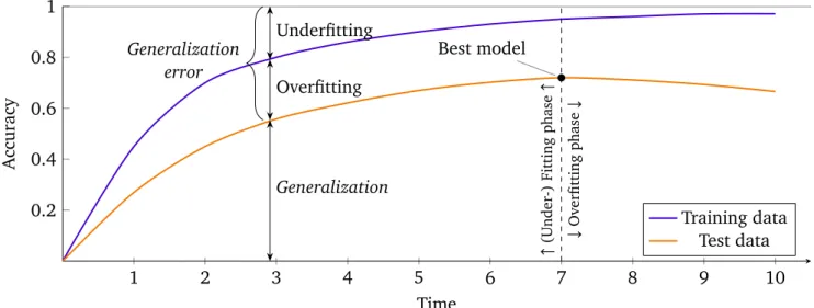
Figure 2.2.:Generalization behavior visualized in the learning curves regarding the accuracy metric on the training data (purple curve) and test data (orange curve) over the course of training. Additionally, the gaps between curves and axes are labeled with the common interpretation terminology and the (under-) fitting and overfitting phases are depicted, which are oriented to the iteration where the best model was achieved.

2.1.4 Generalization

The original goal of ML was to learn a function or task automatically without providing further infor-mation about the problem-solving approach. However, this goal is aimed at being achieved implicitly by letting an algorithm learn from (training) data involving the solution (i.e., the desired model output) for an input but no further solving approaches. This inevitably leads to a small but not negligible shift in the formulation of the goal away from the original one. Namely, learning concepts from the (training) data in order to perform well on this very same data whereby we assume that this good performance will remain on unseen data (meaning data which was not involved during training) and consequently solving the original goal implicitly. This capability of transferring the knowledge to unseen data is re-ferred to asgeneralization. To assess the degree of generalization another data set called the test data set, which is independent of the training data, can be used to measure the performance of the model on this data. A typical generalization behavior is plotted in Fig. 2.2 with the learning curves regarding the accuracy metric on the training as well as on the test data over the course of training (e.g., ten training epochs, which means that the training algorithm has processed the training set ten times). The accuracy metric measures the relative amount (in relation to the number of samples in the data set) of correct classifications on the given data set.

The generalization (of the model), depends on (a) the model, (b) the learning algorithm and (c) the training data. Concerning the model (a), the capacity and expressive power of the model is crucial to capture the concept and patterns of the training data in order to achieve the task. The capacity of a model is usually expressed in the number of parameters and whenever the capacity is too low or the expressive power is improper (e.g., trying to separate the data by a linear model but the data is non-linearly separable only) in order to capture the concept the problem ofunderfitting occurs. Apart from that, the problem of underfitting can also occur when iterative learning algorithms, such as those for learning neural networks, are stopped prematurely whereby the model has not run sufficiently many iterations to fit on the training data properly. Underfitting can be seen in the gap between the accuracy

on the training data and the optimal accuracy value (commonly 1.0). Ensuring a proper expressive power and increasing the capacity of the model addresses the problem of underfitting in most cases but depending on the choice of the learning algorithm (b) this is prone to overfitting. Overfitting can be seen as the gap between the performance on the training data and the test data. This is very dependent on the chosen learning algorithm as, for example, if the model fits the training data (which shows that the capacity is high enough) the model can entirely suffer from overfitting and barely achieves generalization if the learning algorithm encourages rote learning leading to the pure memorization of the training data samples, which is low risk in terms of a low training error but obviously does not serve to generalize the model. Nevertheless, it is common practice especially indeep learningto choose high capacity models while addressing the problem of overfitting with the learning algorithm, i.e., with appropriate regularization techniques (Goodfellow et al., 2016, ch. 7, p. 225) as described in Sec. 2.7 (standard regularization methods) or the novel regularization method introduced in this thesis (see Sec. 3). The suitability of the training data (c) should not be neglected since the success of generalization or even sufficient fitting on the training data hinges with this. Otherwise, the model might tend to overfit to idiosyncrasies of the training data. This is dependent on the amount of data available for training, on the one hand, since a small training set might not be sufficient to recognize general patterns and structures, as well as dependent on the quality of the training data, on the other hand, especially in the case of supervised learning regarding the correctness of the target labels, which were set by humans or even human experts beforehand. Additionally, it is essential to ensure that the distribution and characteristics of the training data match those of the test data or, more generally, match those of the data the learned model is planned to be used on in the future. Furthermore, the samples of the training data have to be drawn independently from the same distribution (in which case the training data and training samples are said to be independent and identically distributed, which is often abbreviated to i.i.d.) (Bishop, 2006, ch. 1.2.4, p. 26).

As one can see in the learning curves of Fig. 2.2, the test accuracy (representing the generalization) is not necessarily asymptotic during learning and can decrease again in a later phase of training. This phase can be denoted as theoverfitting phase whereas the phase before the maximum in the test curve is reached can be called(under-) fitting phase. This is because the model needs some time to learn the general concept and patterns of the data at the beginning of training (fitting phase) while starting to gradually overfit to special samples and idiosyncrasies of the training data later on (overfitting phase). This is the reason why it is advisable to take a snapshot of the best model according to the accuracy (or a similar metric) on some test data over the course of training. After training, this snapshotted model is thebest or most generalized modelachieved during training and is represented by the maximum of the test set learning curve. Within the underfitting and overfitting phases the problem of underfitting and overfitting respectively, is the predominant factor hindering the model from generalizing.

2.2 Artificial Neural Networks

So-called Artificial Neural Networks (ANNs), or also Neural Networks (NNs) for short, can be modestly described as universal, non-linear, and parametric function approximators (Hornik et al., 1989) in math-ematical terms. Since this does not provide an easily understandable introduction to this topic and the name itself is inspired from an entirely different scientific field anyway, we are going to start with a more intuitive perspective: namely from the field of biology or preferably, neuroscience.

Neuroscientific inspiration:

The (human) brain is a huge network consisting of over 120 billion neurons (Herculano-Houzel, 2009) which receive electrical and chemical signals from adjoining neurons and combine those signals by tem-poral and spatial summation. If a unique location, the axon hillock, a swollen part of the cell body of a neuron, is triggered by a charge exceeding a particular threshold a signal is fired on its way to a large number of subsequent neurons (Kandel et al., 2013, ch. 2) known as theall-or-noneprinciple. By doing so, all of these neurons are solving specific tasks by propagating information encoded in the electro-chemical signals step by step where each neuron solves a particular and more simple subtask. Due to the hierarchical arrangement, the brain (a network of neurons) is able to accomplish the whole and more complex task.

The connections between neurons where the transmission of the signals happens are called synapses. The fact that these synapses can transmit the signals to different degrees of effectiveness and, moreover, this modulation behavior of synaptic transmission can change over time, leads to the underlying mech-anism of storing (implicit long-term) memory: a from of learning. This implicit memory storage covers the unconscious and automatic memorization of perceptual and motor skills or habits through habitua-tion, sensitizahabitua-tion, and conditioning, for example. Habituation involves activity-dependent presynaptic depression of synaptic transmission whereas sensitization and conditioning result from presynaptic facil-itation or long-term potentiation of synaptic transmission (Kandel et al., 2013, ch. 66; Chapman et al., 1990). In a nutshell, this type of learning involves changes in the strength of the synaptic signal trans-missions to trigger reactions and behavior that might be advantageous according to the experienced and recurring stimuli.

Note that another type of learning in the human brain exists: the long-term explicit memory storage. This happens consciously like remembering places, objects or people and begins in the hippocampus and medial temporal lobe of the neocortex, which is different from the implicit memorization. Interest-ingly, many skills are initially stored as explicit memory, however, through repetition become ingrained and stored as implicit memory. For example, gradually automating particular finger movements while practicing a piano piece over time (Kandel et al., 2013, ch. 67).

Artificial Neural Networks in computer science:

Now, with this brief biological illustration in mind, we can acquire a mathematical model to approx-imate arbitrary functions by having small units also called neurons doing simple calculations based on numerical input signals with each solving a task partially. They are arranged in a hierarchically struc-tured network by each passing a numerical output signal to subsequent neurons. To achieve an analogy for the modulation behavior of the synaptic transmission effectiveness, real-valued weights are used to scale each input signal. Obviously, by adjusting those weights adequately, the artificial neural network is able to accomplish specific tasks. In order to fit the weights accordingly, automated and data-driven learning algorithms are used in most cases. This process is referred to as learning or, alternatively, as training, optimizing, or fitting the artificial neural network. All of this is explained in more detail in the following sections. However, this is basically the composition of artificial neural networks and holds for many different variants and variations of artificial neural networks developed in the past years.

At this point, it has to be emphasized that – contrary to popular belief often found in the media or popular science – with the use of artificial neural networks we claim neither to simulate the biological brain which is impossible as its functioning is far from being fully discovered yet, nor to offer an adequate or correct abstract model allowing us to draw any conclusions about the brain. By doing so, we would neglect important and strong assumptions since many choices of design and construction are made for mathematical and computational reasons. So the brain should just be seen as an inspiration. In fact,

this is a highly valuable inspiration from which many brilliant ideas and methods have been derived in the past and which drives the research of neural networks further, however it is meant to be no more than an inspiration. Subsequently, and as mentioned above, many techniques were often deduced from mathematics and computer science, making these both essential sources of inspiration and indispensable "toolboxes" in order to get all of this working or even tractable.

The following will examine the concept of artificial neural networks in more detail by starting with the smallest components and ending with advanced architectures.

Early history, in a nutshell:

It all began back to the 1940s with the first theories of biological learning as well as mathematical representations and formal descriptions of neural signal processing (McCulloch and Pitts, 1943; Hebb, 1949; Widrow and Hoff, 1960) moreover with the first breakthrough by Frank Rosenblatt who designed an algorithm called perceptron (Rosenblatt, 1958, 1962) and implemented this on a machine to learn image recognition tasks. 20x20 photocells of a camera were connected randomly to multiple neurons building the single-layer perceptron which was aimed to learn a binary classification of the perceived visual content. As common in ML, in order to learn the task, the perceptron was shown several visual inputs. Whenever theperceptronmisclassified such an input, the weights were adjusted based onHebb’s rule(Hebb, 1949). After the summation of the weighted inputs, theHeaviside step function, which maps negative arguments to zero and non-negative arguments to one (see Fig. 2.8b), was used as activation function in order to produce the final output which was obviously inspired by theall-or-none principleof nervous activity.

Overall, this outstanding work caused a great interest in the field of ML but was later superseded by Marvin Minsky and Seymour Papert in 1969 who showed that aperceptron is not able to represent the logical XOR function (Minsky and Papert, 1969) due to the capability of learning linearly separable patterns only. Later on, it was shown that the logical XOR function can still be learned with a different non-linear choice of activation function (Melnychuk et al., 2017) or the use of a so-called Multi-Layer Per-ceptron (MLP) (with a single hidden layer and non-linear activation functions) which will be explained in Sec. 2.2.3. However, Minsky and Papert (1969) had such a massive impact on neural network research that this stagnated until the 1980s and revived with the invention of the backpropagation algorithm (Rumelhart et al., 1986), explained in Sec. 2.2.4.

2.2.1 The neuron

Nevertheless, the formulation of a neuron as explained in theperceptronalgorithm is still present and is still used in a slightly generalized form in today’s definition of artificial neural networks.

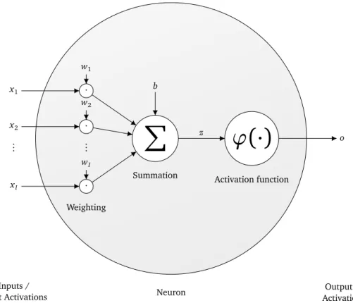
In Fig. 2.3, the composition of an artificial neuron is schematically visualized. Each of the I inputs (also referred to as input activations) the neuron perceives (x₁,x₂, . . . ,x_I) are element-wisely multiplied by the weights (w₁,w₂, . . . ,w_I) in the neuron first. Each weight is exactly assigned to one input at a time which results in the requirement that we always must have as many weights in a neuron as incoming input activations. Inputs, as well as weights, are real numbers with no further restrictions in general.

The weighted input activations are summed up including an additional parameter: the biasb. The bias is independent of the inputs or can also be seen as an additional weightw₀₌ b, which is dedicated to a constant input activation of 1. Obviously, a neuron is a parametric model and the vector of parameters✓ incorporates all the weights and the bias of the neuron. Formally,✓ = (w1,w2, . . . ,wI,b)>. Throughout the training, these parameters are optimized to improve the neuron’s capability to capture the concept of the input and produce the desired output.

To obtain a better understanding of the summation z (called pre-activation) of the weighted inputs it should be mentioned that this weighted sum can also be seen as linear combination of weights and inputs or as the dot product between the vector of the weights w _{= (}w₁,w₂, . . . ,w_I)> _{and the vector of} the inputsx _{= (}x₁,x₂, . . . ,x_I)>_{. Its calculation can be described in matrix-from as follows}

z₌

I

X

i=1

w_i·x_i+b₌w>_{x+b (2.1)}

Up to this point, a neuron is clearly nothing more than a simplelinear modelused in different areas of ML. For example, when solving linear regression each explanatory variable has its own slope coefficient (Freedman, 2009, p. 26) which is equivalent to scaling each input activation x_i by the corresponding weightw_i in a neuron. As the namelinear modelsuggests, this type of model is limited to solve linearly separable problems only. Therefore, we do not use z as the final output of the neuron but apply an activation function (also referred to as transfer function)'first.

Historically, the Heaviside step function as the activation function in the perceptron mimics the all-or-none principle of a biological neuron and the fact that this provides binary instead of real values as output is preferable for binary classification problems. However, the activation function is furthermore of crucial importance in a mathematical context since an appropriate choice serves the capability of a neuron to no longer being limited to separate linearly. Thus, the activation function has to be non-linear, e.g., of sigmoidal shape, a step function, or piecewise linear. The activation function is single-variable and scalar-valued and is commonly of (strictly) monotonically increasing, differentiable, and bounded nature but many well-functioning and widely used activation functions do not meet all of these criteria. Some common activation functions are presented in Sec. 2.4. Note that choosing the identity function '(z) = z as activation function yields a standard linear model as a special case of an artificial neuron. Conversely, an artificial neuron is a generalization of a linear model.

Finally, rather than having multiple input activations, each neuron provides exactly one output acti-vation o. This is merely the result of the activation function o ₌'(z) ='(w>x +b). A more general formulation denoting the output of a parametric model iso₌ f₍x;✓).

2.2.2 Layer of neurons

Up to now, using a single neuron is only capable of producing one output by definition, which at first glance seems sufficient for classification problems or regression problems in ML since there is only one class c ₂ C or one value y 2 Y, respectively, per input sample x desired to be predicted. However, a single output value is not sufficient for regression problems with multiple outputs y ₂ Y ✓ Rn or when the classes in a multi-class classification problem areone-hot encoded. One-hot encoding is always suggested since predicting the class index with a single output value would implicitly lead to learning the misconception about classes whose index values are near to each other that they would be more (semantically) similar to each other than to other ones with more distant index values (as mentioned in Sec. 2.1.1).

For that reason, using several neurons is the most straightforward approach to obtain a model which incorporates the prediction of multiple outputs or, in other words, a vector-valued output

o _{= (}o₁,o₂, . . . ,o_n)> _{instead of a scalar one o. Each neuron receives exactly the same input} activa-tionsx but due to the different weight, as well as bias, values between the neurons, each neuron is able to produce an individual output (activation) o_j. Such a setting is called a layer (of neurons) or also