Automated morphometry for mouse brain MRI through structural parcellation and thickness estimation

(1)

Automated morphometry for mouse

brain MRI through structural

parcellation and thickness estimation

Da Ma

A dissertation submitted in partial fulfillment of the requirements for the degree of

Doctor of Philosophy of

University College London.

Centre for Medical Image Computing Centre for Advanced Biomedical Imaging University College London, United Kingdom

Primary supervisor: Prof. Sebastien Ourselin Secondary supervisor: Prof. Mark Lythgoe

Tertiary supervisor: Dr. M Jorge Cardoso Tertiary supervisor: Dr. Marc Modat

University College London

(2)

I, Da Ma, confirm that the work presented in this thesis is my own. Where infor-mation has been derived from other sources, I confirm that this has been indicated in the work.

(3)

(4)

Abstract

Quantitative morphometric analysis is an important tool in neuroimaging for the study of understanding the physiology of development, normal aging, disease pathology and treatment effect. However, compared to clinical study, image analysis methods specific to preclinical neuroimaging are still lacking. The aim of this PhD thesis is to achieve automatic quantitative structural analysis of mouse brain MRI. This thesis focuses on two quantitative methods which have been widely accepted as quantitative imaging biomarkers: brain structure segmentation and cortical thickness estimation.

Firstly, a multi-atlas based structural parcellation framework has been constructed, which incorporates preprocessing steps such as intensity non-uniformity correction and multi-atlas based brain extraction, followed by non-rigid registration and local weighted multi-atlas label fusion. Validation of the framework demonstrated improved performance compared to single-atlas-based structural parcellation, as well as to global weighted multi-atlas label fusion methods.

The framework has been further applied toin vivoandex vivodata acquired from the same cohort so that the respective volumetric analysis can be compared. The results reveal a non-uniform distribution of volume changes from the in vivo to the post-mortem brain. In addition, volumetric analysis based on the segmented structures showed similar statistical power onin vivoorex vivodata within the same cohort.

Secondly, a framework to segment the mouse cerebellar cortex sublayers from brain MRI data and estimate the thickness of the corresponding layers has been devel-oped. Application of the framework on the experimental data demonstrated its ability to distinguish sublayer thickness variation between transgenic strains and their wild-type littermate, which cannot be detected using full cortical thickness measurements alone.

(5)

pre-sented in this thesis. This demonstrated the successful application of translational quan-titative methods to preclinical mouse brain MRI.

(6)

Acknowledgements

The four years’ PhD study is a precious treasure for me. It won’t be possible without so many kind support, selflessly guidance and continuous encouragement that surrounded me.

Firstly, I would like to thank my primary supervisor, Prof. Sébastien Ourselin, for his valuable advice and guidance throughout my PhD. His continuous support and encouragement also helped me build confidence, learn fast, and develop the courage to tackle challenging tasks.

My gratitude also goes to my secondary supervisor, Prof. Mark Lythgoe, for the various advices he gave me and opportunities he provided that opened my mind and made me learn how to put what I learned into practice.

My grateful appreciation to the two tertiary supervisors in the Centre for Medical Image Computing: Dr. Jorge Cardoso and Dr. Marc Modat, for their thoughtful guid-ance and help throughout my PhD. I’ve learned so much from them through countless discussions.

I would like to thank all my colleagues and friends at CMIC (Centre for Medical Image Computing) and CABI (Centre for Advanced Biomedical Imaging). A lot of the joy of the four years study comes from the beautiful time working together with so many lovely people. Specially thanks to Pankaj and Maria, who shared their valuable experience with me as well as their invaluable jokes, both light and dark; and to Abi, Alex, Carla, Carole, Chris and Jonas for the work, chat and joy we’ve shared together shoulder to shoulder in CMIC; and also to Holly, Jack, James, Ian, Nick and Oz for all the struggling an strive we’ve gone through together as a team in CABI.

I am also very thankful to everyone I collaborated with over these last years within the Centre for Medical Image Computing, the Centre for Advanced Biomedical Imag-ing, the Institute of Neurology, the Crick Institute and the CUBRIC in Cardiff.

(7)

Finally, I want to express my thanks to my dear family members, who have always been along with me. Special Thanks to my cousin Cheng, who studies in the same University as me and makes my study life abroad much more fun. My dearest thanks to my parents, who always bore with me with patience, support and care for me no matter what happened.

(8)

List of Publications

Peer-reviewed Journal Papers

1. D. Ma, M.J. Cardoso, M. Modat, N. Powell, J. Wells, H.E. Holmes, F. Wise-man, V. Tybulewicz, E. Fisher, M.F. Lythgoe, S. Ourselin: Automatic structural parcellation of mouse brain MRI using multi-atlas label fusion. PloS one, 9(1), e86576, 2014.

2. B.A. Duffy, K.P. Chun, D. Ma, M.F. Lythgoe, R.C. Scott: Dexamethasone ex-acerbates cerebral edema and brain injury following lithium-pilocarpine induced status epilepticus. Neurobiology of disease, 63, 229-236, 2014.

3. H.E. Holmes, N. Colgan, O. Ismail,D. Ma, N.M. Powell, J.M. O ´Callaghan, I.F. Harrison, R.A. Johnson, T.K. Murray, Z. Ahmed, M. Heggenes, A. Fisher, M.J. Cardoso, M. Modat, S. Walker-Samuel, E.M.C. Fisher, S. Ourselin, M.J. O ´Neill, J.A. Wells, E.C. Collins, M.F. Lythgoe: Imaging the accumulation and suppres-sion of tau pathology using multi-parametric MRI. Neurobiology of Aging, 2015.

Peer-reviewed Conference Papers

1. D. Ma, M.J. Cardoso, M.A. Zuluaga, M. Modat, N. Powell, F. Wiseman, V. Tybulewicz, E. Fisher, M.F. Lythgoe, S. Ourselin: Grey matter sublayer thickness estimation in the mouse cerebellum. MICCAI 2015.

2. D. Ma, M.J. Cardoso, M. Modat, N. Powell, H. Holmes, M.F. Lythgoe, and S. Ourselin: Multi-atlas segmentation applied to in vivo mouse brain MRI. MICCAI 2012 Grand Challenge and Workshop on Multi-Atlas Labeling.

(9)

1. N. Powell, D. Ma, F. Prados, M. Modat, J. Cardoso, H. Holmes, O. Ismail, N. Colgan, M. O’Neill, E. Collins, M.F. Lythgoe, S. Ourselin: Longitudinal whole-brain atrophy measurement in a mouse model of tauopathy using the Generalised Boundary Shift Integral. ISMRM, 2015.

2. N. M Powell, H. Holmes, D. Ma, M. Modat, J. Cardoso, F. Wiseman, V. Ty-bulewicz, E. Fisher, M.F. Lythgoe, S. Ourselin: Tensor-Based Morphometry re-veals structural differences between Down’s Syndrome and Alzheimer’s disease mouse model brains. ISMRM, 2015.

3. H. Holmes, N. Colgan, O. Ismail,D. Ma, J. Wells, N. Powell, J. O’Callaghan, I. Harrison, M. Cardoso, M. Modat, E. Fisher, S. Ourselin, M. O’Neill, E. Collins, M. Lythgoe: A multi-scale MRI approach to investigate novel drug treatment strategies in mouse models of Alzheimer’s disease. ISMRM, 2015.

4. O. Ismail, H. Holmes, N. Colgan, D. Ma, J.A. Wells, N.M. Powell, J.M. O’Callaghan, I.F. Harrison, S. Walker-Samuel, J.M. Cardoso, M. Modat, E. Fisher, S. Ourselin, T.K. Murray, Z. Ahmed, M.J. O’Neill, R.A. Johnson, E.C. Collins, M.F. Lythgoe: Imaging the accumulation and suppression of tau pathol-ogy using multi-parametric MRI. Alzheimer’s & Dementia 11.7 (2015): P106-P107.

5. J. Steventon, D. Ma, M.J. Cardoso, M. Modat, M.F. Lythgoe, S. Ourselin, R. Trueman, A.E. Rosser, D.K. Jones: A Longitudinal Study In Huntington’s Dis-ease Reveals Differential Macro- and Micro-structural Effects ISMRM, 2014.

6. D. Ma, M.J. Cardoso, M.F. Lythgoe, S. Ourselin: Cortical thickness map: an automatic quantification of cerebral cortex for in vivo mouse brain MRI. British Chapter ISMRM, 2013.

7. H. Holmes, J Wells, N. Colgan, J.M. O’Callaghan, S. Richardson, B. Siow,N. Powell,D. Ma, M. Modat, S. Ourselin, E. Fisher, M. F. Lythgoe: Tensor-Based Morphometry as a Sensitive Biomarker of Alzheimer’s Disease Neuropathology in a Tau Transgenic Mouse ISMRM, 2013.

(10)

8. H. Holmes, N. Powell, J Wells, N. Colgan, J.M. O’Callaghan,D. Ma, M. Modat, M.J. Cardoso, S. Richardson, B.M. Siow, M.J. O’Neill, E.C. Collins, E. Fisher, S. Ourselin, M. F. Lythgoe: Morphometric Genomics: in vivo microMRI for 3D structural imaging of transgenic mice. ISMRM, 2013.

9. D. Ma, M.J. Cardoso, M. Modat, N. Powell, H. Holmes, M.F. Lythgoe, and S. Ourselin: Multi-atlas structural parcellation for in vivo quantification of mouse brain anatomy. British Chapter ISMRM, 2012.

(11)

List of Figures

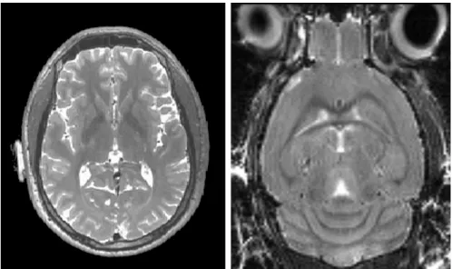
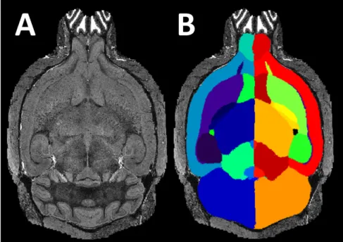
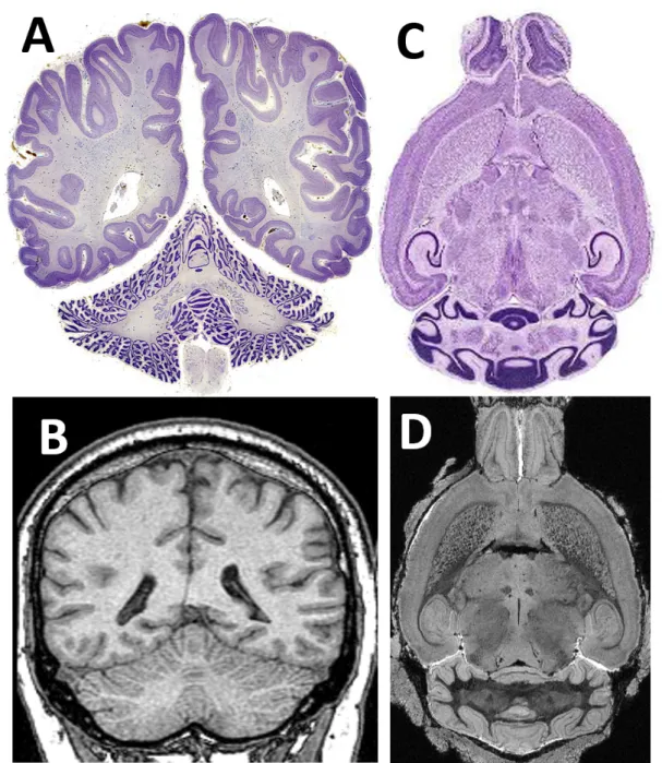
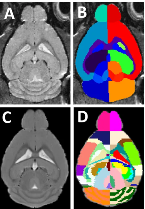
1.1 Comparison of anin vivoT2W of human brain from a 3T clinical scan-ner (Left) and anin vivoT2W mouse brain from a 7T preclinical scan-ner (Right). . . 22 1.2 (A) Anen vivoT2 mouse brain MRI, and (B) It’s corresponding

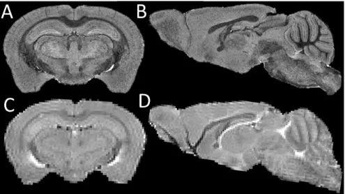
auto-matic structural parcellation result. . . 24 1.3 Top row: (A) coronal view and (B) sagittal view of anex vivoT2 mouse

brain MRI; Bottom row: (C) coronal view and (D) sagittal view of anin vivoT2 mouse brain MRI acquired from the same sample. Theex vivo images have better image quality compared toin vivo image, in terms of resolution, contrast and SNR. It however suffers from post-mortem structural change, such as the collapse of the entire ventricle (the high intensity regions). The parallel stripes appeared in the in vivo image is the truncation (Gibb’s) artifact, which is due to the reconstruction from finite sampled signal in the k-space due to the limited matrix size during the acquisition. . . 25 1.4 Schematic diagram of cortical column architecture, demonstrating

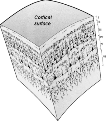
the laminated morphology of the cortical sublayers, with micro-columns passing through the layers perpendicularly. Image taken from NeuWrite San Diego (http://www.neuwritesd.org) . . . 26 1.5 Comparison between human and mouse cortex, both in cerebrum and

cerebellum. . . 28

2.1 Overlapping brain structural tissue intensity histograms of MRI (human brain) make it difficult to distinguish different tissues using only the intensity distribution profile. Figure taken from [1] . . . 31

(16)

2.2 Schematic diagram of atlas-based label propagation . . . 33 2.3 Schematic diagram of multi-atlas structural parcellation. The labels of

each atlas in the database are propagated to the enquiry image through image registration and ranked. A subset of top-ranked atlas candidates are selected and combined through label fusion to obtain the final par-cellation result. . . 36 2.4 Schematic example to shows the parcellation candidate from

single-atlas label propagation (a-c) each with local inaccurate parcellation, but can be fused together with a more accurate consensus final parcellation (d) by locally-weighted label fusion strategy. . . 42 2.5 Schematic graph demonstrating the multistep progressive label

propa-gation. . . 45 2.6 Schematic diagram of different cortical thickness estimation models.

A: Surface based model; B: Voxel-based deformation approach; C: Voxel-based PDE approach . . . 52 2.7 Schematic diagram of the equivolume model for cortical lamination.

The cortical volume is constant across sublayers. As a result, layers with higher curvature becomes thinner. Figure taken from [2]. . . 55 2.8 The uneven distribution of sublayer thickness due to morphological

variation. . . 58

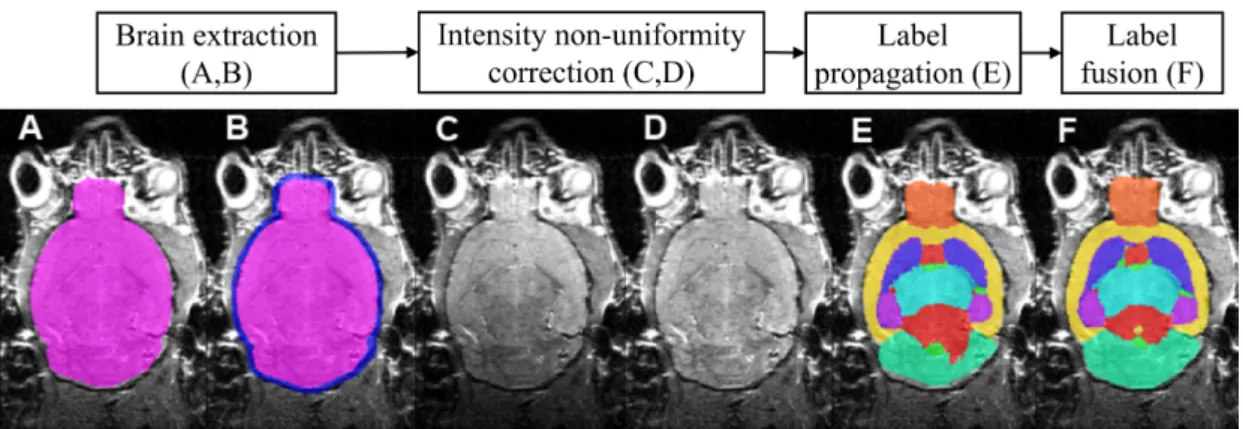
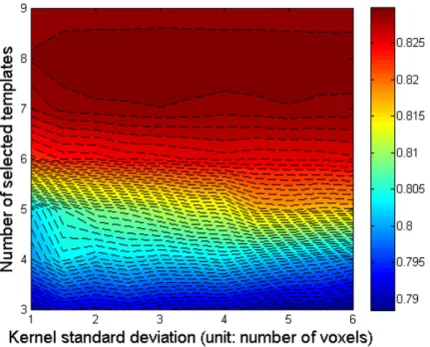
3.1 Step-wise summary of the framework. . . 62 3.2 Sample images of current multi-atlas database . . . 65 3.3 Parameter optimisation for atlas database with left/right hemisphere

separated. . . 71 3.4 Sample images from the cross-validation result of the pipeline on the

atlas databases. . . 72 3.5 Cross-validation result on thein vivomouse brain atlas MRM NeAt [3]. 76 3.6 The structural parcellation result of applying my multi-atlas framework

to a new dataset. . . 77 3.7 Validation of the ability of the multi-atlas framework to parcellate

(17)

3.8 Sample images comparing the parcellation result of the proposed

framework and the single-atlas-based methods. . . 79

3.9 Statistical comparison of the structural volume difference between groups of Tc1 Down’s Syndrome mouse and wild type. . . 80

3.10 Comparison of atlas database with or without flipped atlases. . . 83

3.11 Sample images of each group and its corresponding parcellated struc-tural labels at each time point, and the longitudinal volume change of the region including both hippocampus and cortex. . . 85

3.12 Application of the framework on rat hippocampus segmentation in study drug treatment. . . 86

4.1 Representing images of thein vivoimage andex vivoimage. . . 95

4.2 The structural volumes correlation of thein vivodata versus theex vivo data. . . 96

4.3 Colour-map showing the normalised structural volume difference on each of the corresponding labelled structures. . . 97

4.4 Bland-Altman plot showing the mean proportional volume difference betweenin vivoandex vivomeasurements with regard to the structure size. . . 98

4.5 Statistical comparison ofin vivoandex vivostructural volumetric mea-surement. . . 99

4.6 Statistical analysis to compare the unnormalised individual structural volume of the treated and untreated group on both thein vivo and ex vivodata. . . 101

4.7 Statistical analysis to compare the normalised individual structural vol-ume of the treated and untreated group on both thein vivoandex vivo data. . . 102

5.1 Schematic diagram of the proposed framework. . . 108

5.2 Schematic diagram of the proposed framework. . . 108

5.3 Representative group average image. . . 109

(18)

5.5 Two resistant layers are defined to separate the cerebellar cortical lobes which are not anatomically connected . . . 111 5.6 Two-step extraction of the middle cerebellar Purkinje layer. . . 113 5.7 Iterative multi-kernel Gaussian smoothness gradually recover the

Purk-inje layer. . . 114 5.8 The the accuracy of fissure extraction is improved by removing the

middle Purkinje surface. . . 115 5.10 Normalised grey matter thickness map . . . 118 5.11 Volume of the parcellated grey matter subregions and Surface area of

Purkinje layer. . . 119 5.12 Comparison between the central surface and the Purkinje layer. . . 121

(19)

List of Tables

2.1 Current publicly available mouse brain MRI atlas database. . . 48

3.1 Structural label correspondence between MRM NeAt atlas and NUS atlas. . . 68 3.2 Statistical significant result of the volumetric comparison between the

TC1 groups and wild type. . . 81

(20)

Introduction

Noninvasive medical imaging techniques, such as Computed Tomography (CT), Mag-netic Resonance Imaging (MRI), Positron Emission Tomography (PET) and Single-Photon Emission Computed Tomography (SPECT) allow us to “visualise” the inside of the body noninvasively by collecting signals that represent intrinsic physical, chemi-cal or biologichemi-cal properties of its tissues, and reconstructing those signals into human or computer interpretable images. Depending on the source of the obtained image signal, the medical image can be categorised into structural and functional imaging. Specif-ically, modern neuroimaging techniques provide vast information about the nervous system (mainly the brain), such as the water (proton) density, tissue microstructure, nerve cell myelination, metabolism status, etc. Understanding this information can help us track the development, aging, pathological processes in the brain, as well as response to treatment.

The signal difference between neighbouring tissues or structures with different properties creates image contrast which can be used in image analysis for finding tis-sue/structural boundaries. The longitudinal change of signal intensities is an indication of underlying tissue property change with time in response to pathological, physio-logical or treatment effects. However, it is not a trivial task to interpret the complex information embedded in various types of neuroimages. Proper strategies have to be developed to analyse imaging data accurately and robustly, and extract the appropriate information of interest.

Among various imaging techniques, magnetic resonance imaging (MRI) is often the method of choice because of its soft tissue contrast. In order to detect structural variations among different pathophysiology, or longitudinal structural changes across

(21)

time, it is necessary to have automated and accurate quantitative morphometric analyses of the MR images. Various quantitative morphometric methods have been developed as surrogate biomarkers for image-based diagnosis, such as structural volume analysis, voxel-level morphometry [4], statistical shape analysis [5, 6], boundary shift integral [7, 8] and cortical thickness analysis [9].

1.1

Challenges of brain morphological analysis for

pre-clinical neuroimaging

Genetically modified mice are widely used in preclinical studies of human diseases as they share more than 85% of their genes with humans [10]. As a result, mice are usually the animal model of choice in preclinical research for studying human diseases because of the similar biochemistry and physiology properties they shared with humans, limited variation between inbred individuals, as well as their fast growth and reproduction rate. Since the completion of mouse/human genome sequencing, research focus has been shifted from genotyping to phenotyping, which focuses on the characterisation of var-ious physiological properties expressed by specific functional genomes. Huge efforts have been made involving large scale and collaborative works. Examples of these ef-forts are consortia such as International Mouse Phenotyping Consortium (IMPC1[11]), EuroPhenome2and EMPReSS3[12]. Neuroimaging is a standard technique in clinical environment for disease screening, diagnosis and prognosis, as well as for treatment monitoring, and has also become one important method for phenotyping studies.

Several difficulties arise when imaging small animals in preclinical studies that are not present when imaging humans. These include limited image resolution, signal-to-noise ratio (SNR) and image contrast which are due to much smaller brain size, as well as less control of image artefacts such as motion and flow [13, 14, 15]. With the devel-opment of high field MRI (7-16.4 Tesla compared to clinical MRI which is most com-monly 1.5T and 3T) [16, 17], the advancing of coil and sequence design [18], improved anesthesia techniques [19] and contrast enhanced techniques [20, 21], small animal MR imaging using genetically modified mice has grown rapidly in recent years, and

1_{http://www.mousephenotype.org} 2_{http://www.europhenome.org} 3_{http://empress.har.mrc.ac.uk}

(22)

has been widely adopted as an important tool to study the physiology of diseases’ onset and progression, as well as to monitor recovery outcomes following potential treatment. This is especially the case for neurodegenerative diseases such as Alzheimer’s disease, Huntington’s disease and Down’s syndrome. Fig 1.1 compares thein vivoT2 MRI of a human (acquired with a standard 3T clinical scanner) and a mouse brain (acquired with a 7T preclinical MRI scanner). There is good image contrast in both images to dis-tinguish brain structures as well as to drive the image registration. The partial volume effect is more prominent for mouse brain due to the relatively limited image resolution. The problem is however partially reduced by the lack of convoluted cortical regions.

Figure 1.1:Comparison of anin vivoT2W of human brain from a 3T clinical scanner (Left) and anin vivoT2W mouse brain from a 7T preclinical scanner (Right). The image of human brain MRI is taken from the Alzheimer’s Disease Neuroimaging Initia-tive (ADNI) [22], and the mouse brain MRI is obtained from the study presented Chapter 4.

Despite the continuous efforts to improve the data acquisition, research on anal-ysis for preclinical image studies is still relatively sparse compared to that for clinical studies. With the ever increasing amount of preclinical data, there is a strong and ur-gent need for proper tools that are tailored specifically for preclinical image data to achieve high throughput automated image interpretation and analysis for phenotyping studies [23].

(23)

1.2

Brain image structural parcellation

Structural parcellation, sometimes called structural segmentation, is an important initial step in the analysis of brain images, usually structural MR images (e.g. T1 weighted, T2 weighted or proton density images), and is typically required before further mor-phometric analysis (e.g. volumetric, shape and thickness). In the studies including multispectral MRI (e.g. Diffusion MRI and Function MRI) or multiple image modali-ties (e.g. CT, PET, SPECT), parcellation labels from the the structural MRI can be used to define the regions of interest (ROI) in other image types and confine the analysis of effects to relative structures.

Automated parcellation algorithms try to group voxels in brain images into several different anatomically or functionally relevant regions (Fig. 1.2). The most critical in-formation to guide the parcellation is the image contrast, where neighbouring anatomi-cal structures possess distinguishable signal intensities reflecting the underlying tissue property disparity (e.g. subcortical structures or hippocampus subregions). Other crite-ria have to be adopted in cases where no apparent image contrast is available between neighbouring structures. For example, the boundaries between distinct functional cor-tical subregions are determined from the underlying anatomical morphologies such as cortical gyri and sulci. In cases where there is no image feature to distinguish struc-tures, the structural boundaries can be inferred from other image modalities in which boundaries are visible, e.g. histological slides stained by immunohistochemistry.

Generally, manual parcellation from expert human raters is considered to be the gold standard, and the goal of automatic structural parcellation is to achieve accuracy approaching that standard. Prior information such as anatomical locations (i.e. brain structural atlas) and intensity distribution (i.e. tissue prior maps), are necessary to train the algorithm properly. Various studies have been conducted to improve the struc-tural parcellation accuracy with different approaches. Details of these approaches and current progress on mouse brain image structural parcellation will be reviewed in this thesis, and the application of the automated structural parcellation method to preclinical neuroimages will be explored.

(24)

Figure 1.2:(A) Anen vivoT2 mouse brain MRI, and (B) It’s corresponding automatic struc-tural parcellation result.

1.3

Comparing

in vivo

and

ex vivo

images

When designing preclinical neuroimaging experiments, a crucial choice to make is whether to image the animals alive (in vivo) or postmortem (ex vivo). Imaging the ani-malin vivocan ensure a better preservation of tissue properties and enables monitoring of longitudinal morphological changes; it does however, suffer from limited image res-olution as well as motion and flow artefacts. On the other hand, theex vivoimaging can guarantee higher image quality because of the prolonged motion-free acquisition time and much reduced physiological artefacts; but it suffers from tissue degradation and morphological changes after animal sacrifice as well as experimental procedures such as perfusion and fixation (Fig. 1.3). Currently, it is not entirely clear whether those ad-vantages and drawbacks would affect the quantitative morphometric analysis of brain structures in preclinical neuroimaging. This issue will be explored in this thesis, specif-ically focusing on the effect on the structural volumetric quantification by adopting the framework I developed.

1.4

Cortical thickness measurement

Volumetric measurement is the most fundamental and commonly used imaging biomarker based on structural parcellation. Other quantitative biomarkers are also

(25)

be-Figure 1.3:Top row: (A) coronal view and (B) sagittal view of an ex vivo T2 mouse brain MRI; Bottom row: (C) coronal view and (D) sagittal view of anin vivoT2 mouse brain MRI acquired from the same sample. Theex vivoimages have better image quality compared to in vivo image, in terms of resolution, contrast and SNR. It however suffers from post-mortem structural change, such as the collapse of the entire ventricle (the high intensity regions). The parallel stripes appeared in thein vivo image is the truncation (Gibb’s) artifact, which is due to the reconstruction from finite sampled signal in the k-space due to the limited matrix size during the acquisition.

ing investigated to study more specific morphological properties. Cortical thickness is one of the widely adopted measurements among them.

The cortex is a thin laminar structure of grey matter covering the outermost area of the brain, both in the cerebrum and cerebellum. Research into cortical cytoarchi-tecture has revealed that the cortex is a laminar structure [24, 25]. The neocortex, which is the major part and phylogenetically newest part of the cerebral cortex, con-sists of six cortical layers [25, 26, 2], while the cerebellar cortex concon-sists of three cor-tical layers [27]. According to various studies of developmental and comparative neu-roanatomy, the primary functional units of the cortex are the cortical microcolumns (or minicolumns) that run orthogonal through the cortical layers (Fig 1.4) [28, 25, 29, 30], which varies in function and morphology across different cortical areas due to different neuronal subtypes [31, 32, 33]. Based on this understanding of the cortical micro-cytoarchitecture, researchers have constructed mathematical models of cortical ness from MRI [34, 35, 33, 36, 2, 37]. The morphological variation of cortical thick-ness, at both the global and local scale, has been shown to be associated with various neurodegenerative diseases [38, 39, 40, 41, 42].

(26)

Figure 1.4:Schematic diagram of cortical column architecture, demonstrating the lam-inated morphology of the cortical sublayers, with microcolumns passing through the layers perpendicularly. Image taken from NeuWrite San Diego (http://www.neuwritesd.org)

The WM/GM ratio of human is much larger than that of the mouse, as the axons increase disproportionally faster than the neocortex during revolution [43], and the hu-man cortex is more convoluted both in cerebrum and cerebellum. Meaningful cortical thickness measurement relies on accurate cortical extraction, so that the inner and outer boundaries of the cortex can be accurately defined from the surrounding tissues. How-ever, the accuracy of the cortical surface extraction is hindered by the partial volume effect due to the cortical convolution, as well as the thin nature of cortex, (2-3mm for normal healthy human cortex vs. 1mm voxel resolution for standardin vivoMRI, and 200-400µm for normal wildtype mouse cortex vs. 150µm voxel resolution for standard in vivoMRI and 40µm voxel resolution for standardex vivoMRI). A proper model of the cortical thickness, such as the cortical layers and microcolumn structures, is neces-sary to make an anatomically plausible measurement.

The human and mouse cortices have a distinctive morphology, both in cerebrum and cerebellum, as shown in Fig. 1.5. In human, current standard MRI is able to capture the morphology of sulci and gyri in the cerebral cortex, but not those in the cerebellar

(27)

cortex, which is more convoluted (Fig. 1.5A,B). Compared to that of the human, the mouse cerebral cortex is almost flat, which makes it relatively easier to extract and quantify. The mouse cerebellum is also less convoluted than human cerebellum, and can be well captured by ex vivo MRI (Fig. 1.5C,D). In addition, different cell layers in the mouse cerebellar cortex are also observable in the corresponding MRI, which makes it possible to investigate the cerebellar cortical sublayer quantitatively. It would be ideal to incorporate such image-contrast-based layer information into the cortical thickness model, and estimate the sublayer thickness of the mouse cerebellum.

1.5

Genetically modified animal models

To validate the translational frameworks I developed and presented in this thesis, mouse brain image data acquired from two inbred strains of transchromosomic/transgenic mice were used. The strains respectively model two neurodegenerative diseases: Down’s Syndrome (DS) and Alzheimer’s disease (AD). For the sake of the complete-ness, a description of these two mouse models is provided here.

Firstly, the Tc1 mouse model - a transchromosomic mouse strain that models Down’s syndrome (DS) - was used in the validation of structural parcellation (in Chap-ter 3) as well as the cerebellar cortical sublayer thickness estimation (in ChapChap-ter 5). The Tc1 mouse line is a trans-species aneuploid model of mouse carrying a freely seg-regating copy of human chromosome 21 (Hsa21) and thus is functionally trisomic for 75% of Hsa21 genes, which has the clinical manifestation and similar phenotypes of DS in humans [44, 45].

The rTg(TauP391L)4510 mouse model for human tauopathy was used to compare volumetric analysis usingin vivoandex vivoimaging (in Chapter 4). rTg4510 mouse overexpresses the tau protein (4R0N) due to the mutation (P301L) in exon 10. This abnormal processing of tau will lead to the neurofibrillary tangles (NFTs), which is associated with Alzheimer’s Disease (AD) and other neurodegenerative diseases such as Parkinson’s disease and frontotemporal dementia [46]. In the rTg4510 model, the transgene overexpression is induced through the Tetracycline-controlled transcriptional activation, a reversible gene transcription method in which the level of overexpression can be controlled through the treatment of doxycycline.

(28)

Figure 1.5:Comparison between human and mouse cortex, both in cerebrum and cerebellum. (A) A slide of the human brain with hematoxylin and eosin (H&E) stain at the axial view. (Image taken from the “The Human Brain Atlas” at: http://www.msu.edu) (B) Anin vivoMRI of human brain at similar slice position. (Image taken from the “The whle brain atlas” at: http://www.med.harvard.edu/aanlib/) (C) A slide of the mouse brain with hematoxylin and eosin (H&E) stain at the sagittal view (Image taken from www.neura.edu.au) (D) The corresponding sagittal view inex vivoMRI of mouse brain.

1.6

Thesis contributions

The aim of this thesis is to develop automated quantitative structural analysis frame-works for mouse brain MRI, which can be used to study the pathology of

(29)

neurodegen-erative diseases and the effect of potential treatments. Specifically, this thesis focuses on the construction and validation of two quantitative methods - brain structural parcel-lation and cerebellar cortical sublayer thickness estimation.

• Firstly, a multi-atlas-based structural parcellation framework is constructed. The framework incorporates preprocessing steps such as intensity non-uniformity correction and multi-atlas-based brain extraction, followed by label propagation based on non-rigid registration and locally weighted multi-atlas label fusion. The parameters in the label fusion step are optimised through leave-one-out cross val-idation, and the parcellation framework is evaluated on bothin vivoandex vivo MRI data. This is the first multi-atlas-based brain parcellation framework applied on bothin vivoandex vivomouse brain MRI. The proposed framework outper-forms single-atlas-based structural parcellation, as well as global-weighted multi-atlas label fusion algorithm. When applied to the ex vivo images of a Down’s Syndrome mouse model, the proposed framework also successfully detects phe-notypes in terms of structural volumetric difference between groups with differ-ent genetic backgrounds.

• To provide some quantitative guidance for the experimental design of small ani-mal neuroimaging studies, I applied the structural parcellation framework to both thein vivo and ex vivodata acquired from the same wildtype cohort, and com-pared the volumetric analysis result of the two measurements. The results showed a non-uniform distribution of brain volume shrinkage fromin vivotoex vivodata. When determining the effect of a treatment compound, bothin vivoandex vivo images demonstrated similar statistical analysis result using the parcellated brain structural volumes as a quantitative biomarker.

• Based upon the structural parcellation, a multi-layer thickness estimation frame-work is developed for morphometric characterisation of mouse cerebellar corti-cal sublayers from the high-resolution, contrast-enhancedex vivoMRI. A layer model which follows the laminar features of the highly convoluted cortex is adopted which, when combined with an anisotropic contrast enhancement filter, segments and estimates the thickness of the cerebellar sublayers. Evaluation of the framework on mouse models of Down’s syndrome demonstrated its ability to

(30)

detect regional cortical sublayer thickness variations, which cannot be revealed using full cortical thickness measurements alone.

1.7

Thesis organisation

This thesis introduces the development and translational applications of two quantita-tive medical image analysis frameworks I developed in my PhD: the automated struc-tural parcellation for volumetric analysis, as well as thickness estimation for cerebellar cortex.

Chapter 2 presents a literature review about the current state-of-the-art in auto-mated structural parcellation and cortical thickness measurements, both in clinical and preclinical scenarios. I also review the current research on the relation between the structural analysis ofin vivoandex vivoimages.

Chapter 3 presents a multi-atlas structural parcellation framework for mouse brain MRI. The framework is evaluated on various datasets, both in vivoand ex vivo data. This chapter also demonstrated the successfully application of the framework in different studies.

InChapter 4, the structural parcellation framework is applied to compare the vol-umetric analysis on images acquired eitherin vivoorex vivofrom the same cohort. The evaluations include both direct comparison of volumetric analysis and the application of the framework to discriminate between two animal groups.

InChapter 5, a framework of cerebellar subcortical layer segmentation and thick-ness estimation is introduced. This incorporate both intrinsic image contrast and a mathematical model of the cortical lamination. The framework is validated on theex vivomouse brain MRI.

Finally, an overall discussion is presented in Chapter 6, and the thesis is con-cluded in Chapter 7, in which the plan for the future direction of my work is also discussed.

(31)

State-of-the-art

2.1

Automatic structural parcellation for mouse brain

Structural parcellation is the process of extracting the labels of brain structures from images like MRI, CT, ultrasound, etc. In medical images, different anatomical struc-tures might share similar tissue intensity properties, and the same structure may contain several different tissue classes (Fig. 2.1) [1]. As a result, it is not possible to parcel-late brain structures automatically based solely on the tissue intensity distribution as in brain tissue segmentation - a process in which the brains are segmented into grey matter (GM), white matter (WM) and cerebralspinal fluid (CSF). Manual labeling by experts is still the current gold standard of structural parcellation in MRI studies of mouse brains, despite being expert-dependent and labour intensive [3, 47].

Figure 2.1:Overlapping brain structural tissue intensity histograms of MRI (human brain) make it difficult to distinguish different tissues using only the intensity distribu-tion profile. Figure taken from [1]

(32)

2.1.1

Atlas-based label propagation

There are two types of structural information that can be derived from MRI images: shape- (or edge-) based labels and volume- (or voxel-) based labels. The shape-based labels define structures with a contour or mesh based labels, sometimes along with vari-ous visual appearance feature statistics. Several methods have been developed to extract the shape information of one or several structures, such as hippocampus and cerebel-lum, for rodent brain through active shape model [48], active appearance model [49, 50] and active volume model [51]. This type of automated structural extraction technique shows promising result to segment some specific structures. Its performance is how-ever relying on the image gradient information which is sensitive to noise and spurious edges. As a result, using the shape-based method along is inadequate to simultaneously parcellate large number of structures with variable size and shapes as well as structures with complex intensity distribution profile.

Another type of structural information is voxel-based structural labels, where all the voxels in the same structure are assigned the same label. The manually delineated structural labels for existing MR images can be used as prior information to automat-ically parcellate new images, in a process called atlas-based label propagation. Here an atlas is defined as a pair of images containing both the original MR data (either from a single sample or a groupwise average) and its corresponding manually labelled anatomical structures. The atlas based label propagation method has shown parcellation accuracy when compared to manual labeling for both clinical [7, 52] and preclinical im-ages [53, 54]. There are increasing number of brain atlas databases developed and re-leased for human brain [55, 56, 57, 58, 59, 60, 61, 62, 63, 64, 65, 66, 66, 67, 68, 69, 70] and for mouse brain [71, 72, 73, 74, 75, 76, 77, 78, 3, 79, 47, 80, 81, 82]. A typi-cal atlas-based label propagation consists of two steps: image registration and label propagation (Fig. 2.2).

Image registrationAtlas-based label propagation relies on image registration, which is one of the fundamental techniques in medical image processing (Fig. 2.2). In image registration, a transformation matrixT which deforms a floating imageIF to the space of a reference image I_R is optimised to minimise the image differences (or maximise image similarities depending on the objective function adopted) between the deformed floating imageT(I_F)and target imageI_T (Fig. 2.2 1 ).

(33)

Figure 2.2:Schematic diagram of atlas-based label propagation. The template image from the atlas is firstly registered to the enquiry image. The resulted deformation matrix is then applied to the atlas labels to derive the structural parcellation result.

When performing the image transformationT, the deformed floating imagesT(I_F) are resampled into the space of the reference image I_R: ∀~x∈T(I_F). The intensity of T(I_F)is calculated at its corresponding coordinates (determined fromT) in the space ofI_F through intensity interpolation (e.g. linear, spline, sinc, etc).

Current state-of-the-art image registration framework normally involves two steps: the global-transformation-based step followed by a local-transformation-based step [83]. In the global registration step, the same image transformationT is applied to each pixel (in the case of 2D) or voxel (in the case of 3D) in an image, by ei-ther rigid transformation (including translation and rotation) or affine transformation (adding shearing and scaling to a rigid transformation). In the local (also called elastic or non-rigid) registration step, a deformation field which is capable of performing local wrapping is generated to account for the unevenly distributed local image dissimilarities through either parametric or non-parametric deformation models [84]. Regularisation or penalty terms are used to ensure a smooth deformation and anatomical plausibility.

Label propagationAfter the deformation field is determined through image registra-tion, the same transformation is then applied to the manually labelled anatomical struc-tures in order to match the unlabelled image’s morphology (Fig.2.2 2 ). To preserve the integral nature of the resulted label, the resulted labels are resampled through near-est neighbour interpolation, in which the label values were determined from its

(34)

corre-sponding coordinates (determined fromT) in the space of atlas label L_F similar to the interpolation procedure in the registration steps, but are assigned the label value of the voxels inL_F that have the shortest distance to the transformed positions.

As the performance of structural parcellation is directly related to the image reg-istration accuracy, this single-atlas label propagation technique is also referred to as registration-based structural parcellation. Leeet al.[53] evaluated two different non-rigid registration algorithms to achieve label propagation on mouse brain, the fluid-model [85] and free-form B-spline[86], and found a similar performance both in terms of accuracy and stability. However, although image registration algorithms are con-stantly advancing, it is by itself an ill posed problem [87]. Compared to human pa-tients, the subject variations within same mouse strains is relatively small. However, local misalignment will still occur due to the large morphological variability across strains, imaging artefacts, low signal-to-noise-ratio (SNR) or contrast-to-noise ratio (CNR), resulting in poor parcellation accuracy.

2.1.2

Probabilistic-atlas-based structural parcellation

To account for the morphological variation within populations, probability-based atlas priors have been proposed instead of discretised ones, where the probability represents the occurrence of different labels for each voxel.

Scheenstra et al.[88] parcellated the structures from mouse brain MRI through an edge-based Bayesian clustering after single-atlas label propagation using only affine registration. The algorithm uses prior information derived from the atlas regarding the intensity distribution within each label class to guide the edge-based Markov Ran-dom Field (MRF) clustering on the query image. Evaluation of the algorithm in bothin vivoandex vivomouse brain images showed comparable performance to par-cellation methods based on non-linear registration [89]. This edge-refinement meth-ods reduced the required computational time significantly compared to non-linear-registration-based parcellation, while maintaining comparable parcellation accuracy. However, this method requires a reasonable initialisation from affine registration, and therefore cannot account for large local morphological variations between the atlas and query images. The statistical prior information also relies on a similar intensity distri-bution between the atlas image and the query image, which is not always the case.

(35)

Aliet al.[90] developed an automatic parcellation framework using multi-spectral MR microscopy (including T2, proton density and diffusion weighted images) for the mouse brain, which is a follow up to the previous study on human brain MRI by Fis-chlet al.[1]. The probabilistic atlas database is constructed from 6 intensity-normalised brain images affinely registered to a common space, each with 21 manually labelled structures. The intensity information from the multispectral MR images forms a multi-dimensional feature space, and is modelled as classes of multivariate Gaussian distribu-tion. The contextual information is modeled under a spatially variant first-order MRF model. The final labels are obtained through maximum a posteriori (MAP) estimation. This framework has been applied to mouse brain MRI with image contrast enhanced by active staining technique [91] to characterise the intra-strain [92], and inter-strain [93] structural volumetric variation. However, the multispectral imaging protocols increase the scanning time, making them unfeasible for use in all studies.

Baeet al.[94, 95] and Wuet al.[96] extended this model by adopting a support vector machine (SVM) classifier (which has been extended to multiclass classification) to model the posterior label probabilistic function instead of using the Gaussian prob-ability distribution. This extended MRF outperforms the original methods proposed by Aliet al.[90] when evaluated on the same multispectral data, but requires a much longer training time. (For a training dataset of 5 mouse brains manually segmented into 20 structures, it tooks 290 to 364 minutes to train the algorithm excluding the registra-tion time, and 75 minutes to segment one brain, on a 3.4-GHz PC.) This however is not a big problem if the training set is fixed, as the training procedure only need to be performed once offline.

Compared to the registration-based single-atlas label propagation, the probabilistic-atlas-based structural parcellation demonstrated improved accuracy, especially with the help of MRF to consider contextual voxel information. However, this probabilistic ap-proach still can not fully capture large local morphological variations across subjects, and the improvement over small-structure parcellation is still limited.

2.1.3

Multi-atlas label propagation and fusion

With the availability of the database which contains more than a single atlas, another ap-proach has become increasingly popular recently which improves the structural

(36)

parcel-lation accuracy by combining information coming from multiple atlases in a database into a consensus result - a method normally called “label fusion” (Fig. 2.3) [97, 98, 99]. This multi-atlas label fusion approach has gained increasing attention in recent years due to its promising performance, and has multiple applications in both clinical and preclinical neuroimaging [100].

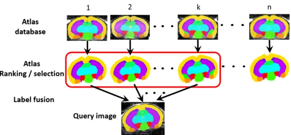
Figure 2.3:Schematic diagram of multi-atlas structural parcellation. The labels of each atlas in the database are propagated to the enquiry image through image registration and ranked. A subset of top-ranked atlas candidates are selected and combined through label fusion to obtain the final parcellation result.

In a multi-atlas structural parcellation, the first step is to perform image registra-tion and label propagaregistra-tion for each individual atlas in the database as in the single-atlas-based method. The propagated structural label candidates are used as a training set to obtain the best final structural label for the query image (rather than treat the candidates equally as in the probabilistic atlas). Fig. 2.3 shows the basic workflow of a label fusion algorithm. The performance or accuracy of the candidate labels are first estimated or ranked (either globally or locally). A subset of top ranked labels are then selected and combined to estimate the underlying true structural labels.

2.1.3.1

Majority voting

An intuitive way to fuse the labels is through majority voting, in which each voxel is assigned to the label that receives the largest number of votes from the propagated candidate atlases [101, 102]. Suppose there areNatlases in the database, and we denote Sn as the structural parcellation candidate for each registered atlas template image, wheren∈1...N. Forx∈ΩwhereΩis the computational domain in the query image

(37)

space, the final labelS(x)can be obtained from: S(x) = arg max l∈{1,...,L} N

∑

n=1 1 Np(l|Sn,x), (2.1) whereLis the total number of labels, p(l|Sn,x)is the probability of parcellation can-didate S_n vote for label l at voxel x, which is 1 if S_n(x) = l and 0 otherwise, and

∑Ll=1p(l|Sn,x) =1∀n∈1, ...,N.

Given the fact that the propagated parcellation of some atlas templates performs better than others, studies have been focused on ranking the atlases in order to assign different weights to them during the label fusion process, or only select a small subset of atlases with higher rank for label fusion, to improve the parcellation accuracy. The updated voting equation becomes:

S(x) = arg max l∈{1,...,L} N

∑

n=1 wn(x)p(l|Sn,x), (2.2)

in which thew_n(x)is the assigned weight to thenthatlas, where∑N_i₌₁wn(x) =1. The weightw can be simple metadata [103], such as age or sex [104], or can be the image similarity between transformed atlas and the test image using methods such as Summed Square Distance (SSD) [105], Mutual Information (MI) [106], Normal-ized Mutual Information (NMI), or transforming distance [107, 108]. Wuet al.[104] attempted to find the single most appropriate atlas within the database through the NMI image similarity measurement, and demonstrated improved parcellation results. Wang et al. [102] managed to optimise the weight wn(x) by minimising the total er-ror calculated as the correlation between each atlas image and the query image in a covariance matrixMxand solved through a Lagrange multiplier.

2.1.3.2

Atlas selection

Besides weighting, studies have managed to select limited atlases from the database based on different ranking scheme and demonstrated improved parcellation accuracy. Aljabar et al. [109] selected the atlas subset randomly without ranking, and showed that the accuracy of the majority voting label fusion depends on the number of atlases selected, but reaches the plateau when the number of atlas selected reaches a certain number. Wu et al. [104] selected the single best template (determined by measuring

(38)

the NMI between the registered atlas image and the query image) within the database and achieved a parcellation accuracy better than simply averaging all the parcellation. Aljabaret al.[103] later demonstrated that the label fusion accuracy can be significantly improved by using a subset of best ranked candidate labels, with the atlases ranked by the global normalised cross correlation (GNCC) between the registered template and the query image over a specific region of interest. Sabuncuet al. [105] extended the study by Aljabaret al.[109] and concluded that, when selecting the top ranked atlases instead of selecting them randomly, the parcellation accuracy is less dependent on the number of atlas selected. Shenet al.[108] suggested another atlas ranking scheme us-ing the Least Angle Regression (LAR), a variable selection method in regression, and demonstrated improvement in both parcellation accuracy as well as robustness when compared to the other ranking scheme using image-similarity-based measurement in-cluding NMI, cross correlation (CC), and Mean Square Difference (MSD).

2.1.3.3

Selective and Iterative Method for Performance Level

Estima-tion (SIMPLE)

Compared to image similarity, a better way to compute the weight for the parcellation candidatesS_iwould be estimating the performance of each candidate by calculating its agreement to the underlying ground truth parcellation (e.g. Dice similarity coefficient -DSC, Jacard coefficient, or sensitivity and specificity). Although this performance level is not readily available due to the lack of such ground truth, it can be approximated as the current estimation of the fused label and improved iteratively.

Langerak et al. [110] devised an algorithm - Selective and Iterative Method for Performance Level Estimation (SIMPLE) - which combines the advantage of both at-las selection and performance estimation in an iterative manner and showed further improvement in parcellation accuracy. In the SIMPLE algorithm, the initial true par-cellation estimation S0_T is obtained from weighted majority voting, with the weight determined from NMI. At each iteration j, the performance of each parcellate candi-dateSi is calculated as the binary label overlap measureE(Si,S_Tj). A subset ofSiwith performance above a thresholdE(S_i,S_Tj)>θjare selected to estimate the updatedS_Tj+1

using weighted majority voting weighted byE(Si,S_Tj)untilST converges. The thresh-old at iteration j is determined as: θj=µj−α×σj, where µj andσj are the mean

(39)

and standard deviation of the performance of all the parcellation candidates, andα is a

scalar variable which controls the number of candidates discarded in each iteration.

Leave-one-out validation on the SIMPLE algorithm demonstrated promising per-formance, which is not sensitive to the choice of either the performance estimator or the initial estimation of the true parcellation S0_T. However, the fact that the underly-ing true parcellation is determined based on weighted majority votunderly-ing from the current available parcellation candidates is not perfect, which will incur bias when calculating the subsequent parcellation performance.

2.1.3.4

Simultaneous Truth and Performance Level Estimation

(STA-PLE)

Warfieldet al.[98] developed an algorithm - simultaneous truth and performance level estimation (STAPLE) - which fuse a set of structural parcellation candidates of a test image (from either expert labelling or automatic label propagation algorithm) by com-puting the probabilistic estimate of the underlying ground truth parcellationST (rather than the actual S_T as implemented in the SIMPLE algorithm [110]). The algorithm treats the ST as missing/hidden data in a complete dataset which includes both the parcellation candidate and the true parcellation: (S₍₁_,...,_N₎,S_T), and optimises the es-timation of ST through an iterative expectation maximization (EM) framework. The EM framework is initialised by assigning equal weights to each parcellation candidate (label assignment), and iteratively updates the sensitivity p (proportion of true posi-tive) and specificity q (proportion of true negative) to obtain the optimal weights to derive the combined parcellation. The performance level here is defined as the pand qof propagated parcellations for each individual atlases. The parameters pand qare defined as the conditional probability:

  

 

pl_n=P(S_n=l|ST =l)(true positive fraction) ql_n=P(S_n6=l|ST 6=l)(true negative fraction)

∀n∈ {1, ...,N}. (2.3)

In order to estimate the optimisedST, it is necessary to maximise the complete dataset

(40)

the cost function of the log likelihood of(P(S₍₁_,...,_n₎,S_T|p,q): (p,ˆ qˆ) =arg max

p,q

log(P(S₍₁_,...,_n₎,S_T|p,q)). (2.4)

With the assumption that the candidate parcellation are independent to each other (thus S_i⊥ S_j, p_i ⊥ p_j and q_i⊥ q_j, ∀i6= j), Eq. 2.4 can be optimised in an Expectation-Maximisation fashion. The posterior probability of a voxel x belonging to label l ∈ {1, ...,L}is denoted asW_l(x)(Expectation step), and is estimated as:

W_li+1≡P(ST =l|S{1,...,N},pi,qi) = α α+β , (2.5) where α =P(ST =l)

∏

n P(Sn|ST =l,pn,qn), (2.6) β =P(ST 6=l)

∏

n P(S_n|ST 6=l,pn,qn). (2.7) And the performance level parameter p, q that maximise the log likelihood of the es-timated underlying ground truth for each labell and each parcellation candidate nare updated in each iteration (Maximisation step):

pi_n+1=∑S=lW i l ∑LWli , (2.8) qi_n+1= ∑S6=l(1−W i l) ∑L(1−Wli) . (2.9)

This expectation-maximisation framework is solved recursively following Bayes’ rule until the final true parcellationS_T converges.

Rohlfinget al.[97] generalised this algorithm to multiple labels fusion by replac-ing the parameters pandqin the original STAPLE algorithm by a “confusion matrix” Mn, an idea introduced by Xuet al.[111], in which each entrymn,i,jinMnrepresent the joint-occurrence of candidate parcellation label decisioni and the corresponding true label j:

m_n,i,j=#{x|Sn=i,ST = j}, (2.10) The sensitivity p_nis equivalent to the corresponding row normalised cross-parcellation

(41)

coefficientλn, and can be computed as:

p_n≡λn=P(Sn(x) =ln|ST(x) =ln) =

m_n,i,j

∑jmn,i,j

, (2.11)

while the specificity qn are spread over the off-diagonal element of Mn and can be expressed as: qn≡1− ∑_i0 6 =imn,i0,i ∑_i0₆ =i∑jmi0,j . (2.12)

Validation of the STAPLE algorithm showed significant improvement of parcel-lation accuracy over voting strategies when applied on digital/brain phantom data [98] and real data acquired and manually segmented from 3D confocal microscopy images of the honeybee brain [112]. Leunget al.[113] applied STAPLE algorithm to brain ex-traction of human brain MRI and demonstrated improvement compared to other frame-works. Leunget al.[114] also demonstrated successful application of STAPLE algo-rithm for hippocampal segmentation, which achieved good distinction between control, mild cognitive impaired patients (MCI) and Alzheimer’s disease patients (AD), as well as the ability to predict disease progression for MCI patients.

2.1.3.5

Locally-weighted label fusion strategies

The parcellation candidates for label fusion come from the registration-based label propagation. The parcellation errors of individual candidates may originate from the lo-cal morphologilo-cal variations, lolo-cally inaccurate registration due to noise or regularisa-tion, or resampling error due to partial volume effect in images with limited resolution. In cases where the registration algorithm performs well in some local regions but poorly in some other regions (as shown in 2.4), a global ranking/weighting is no longer fully representative of the local parcellation quality and sometimes misleading, and may af-fect the final parcellation accuracy. This efaf-fect is more apparent when the number of at-las candidates is limited. Methods have since been proposed to weight and fuse the atat-las locally, thus improving the accuracy of the parcellation compared to globally weighted voting strategies, especially in areas with bad tissue contrast (Fig. 2.4) [115, 105, 102]. Wanget al.[102] introduced a locally-weighted majority voting method and man-aged to reduce the expectation of the combined error correlation between parcellation candidate by optimising the local weight with a neighbourhood specified by a radius

(42)

Figure 2.4:Schematic example to shows the parcellation candidate from single-atlas label propagation (a-c) each with local inaccurate parcellation, but can be fused together with a more accurate consensus final parcellation (d) by locally-weighted label fu-sion strategy.

r through covariance matrix. Agarwal et al. [116] proposed a locally-weighted and multi-label SIMPLE method for Chest CT data by dividing the images into overlap-ping local cubes and deriving different weight to different local regions, which showed improvements over the original SIMPLE algorithm with global strategy. Artaechevar-riaet al.[115] further conducted an experiment to compare the parcellation accuracy by using various global and local fusion algorithms - including majority voting, global weighted voting based on normalised cross correlation (NCC), MI or MSD, locally-weighted voting based on NCC, MI or MSD, as well as STAPLE - and concluded the best label fusion strategy to be the locally-weighted voting based on MSD.

Finally, Cardosoet al.[117] recently proposed an algorithm - multi-label Similar-ity and Truth Estimation for Propagated Segmentations (STEPS) - which incorporates a local ranking strategy for template selection based on a locally Normalised Cross Correlation (LNCC) to the original STAPLE algorithm for atlas selection. STEPS al-gorithm introduces a new image similarity based model variable to represent the ob-served cluster assignmentO(x)which is equal to 1 if the registered atlas imageT(IFn) is within the selected top ranked image at voxel x and equal to 0 if otherwise. The original STAPLE framework (Equation 2.4) is thus transformed to:

(p,ˆ qˆ) =arg max p,q

log(P(S₍₁_,...,_n₎,S_T,O)|p,q))). (2.13)

And the expectation maximisation optimisation scheme in the original STAPLE frame-work (Equation 2.5) now becomes restricted maximum likelihood (REML) which

(43)

fo-cuses only on the likelihood of a subset of the data:

W_l≡P(S_T =l|S_{₁_,...,_N},O=1,pi,qi) = α

α+β . (2.14)

In addition, the STEPS algorithm also integrated the MRF regularisation into the op-timisation scheme that Cardoso et al. previously developed [118] which is updated iteratively with a mean field approximation on the probabilistic labels. This is in con-trast to the MRF regularisation presented in the original STAPLE algorithm, which was implemented as a post processing step. Similarly to Rohlfinget al.[97], Cardosoet al. also extended this “local ranked STAPLE” algorithm to multiple label fusion through a confusion matrixMn (Equation 2.10) and its corresponding row normalised equiv-alent λn (Equition 2.11). Performance validation of the STEPS algorithm on human brain MRI showed significant improvement in parcellation accuracy compared with the ranking using global cross correlation (GCC), and is also less dependent on the size of the atlas database and the number of selected templates [117].

2.1.3.6

Learning-based mislabel correction and joint label fusion

The structural parcellation errors consist of random errors and consistent errors [119, 103, 102]. The random errors normally come from image noise and anatomical varia-tion, and can be reduced through the label fusion methods reviewed above. The consis-tent error is a systematical bias when transferring manual segmentation into automatic segmentation which however, cannot be corrected by the the conventional label fu-sion methods. To address this problem, Wanget al.[102] developed a learning-based wrapper to detect the mislabeled voxels which are affected by the consistent error be-tween the automatic and manual segmentation, and replace that with corrected labels classifier. The classifiers combines the information from of image feature (normalised intensity), contextual feature (label of the neighbouring voxels) as well as coordinate feature (spacial information). Application of this learning-based wrapper on the local-weighted multi-atlas label fusion methods [115, 105] demonstrated a reduction of con-sistent segmentation bias and lower mislabeled voxels.

In addition, within a multi-atlas database, the segmentations from some atlas can-didatesδi(x) are more similar than the rest in the database. Wanget al.[120] further

(44)

when combining labels. Instead of estimating the weight for each atlas independently, the joint label fusion algorithm also calculate the correlation between each atlas pairs, where the pairwise dependency is defined as the joint probability of segmentation er-ror. The total expected errorE between the the consensus segmentationS(x) and the true segmentationS_T(x)is given byE=wT_xM_xw_xwherew_x= [w₁(x);...;w_n(x)]are the estimated weights, and M_x is a pairwise dependency matrix estimating the likelihood that two atlases both produce wrong segmentation:M_x(i,j) =p(δi(x)δj(x) =1). The

voting weights are estimated to minimise the total expectation error, i.e.

w∗_x =arg minwt_xM_xw_xsubject to n

∑

i=1

w_i(i) =1. (2.15)

Validation of the joint label fusion algorithm on hippocampus segmentation and hip-pocampal subfields segmentation showed its ability to eliminate the effect of the redun-dant information from similar atlases when assigning the weight.

The combination of the learning-based mislabel correction and the joint label fu-sion method has demonstrated great segmentation accuracy [121], and the final imple-mentation has won the first place of the MICCAI 2012 Multi-Atlas Labeling Challenge, and is also among the top performers in MICCAI 2013 segmentation: Algorithms, The-ory and Applications (SATA) challenge.

2.1.3.7

Progressive label propagation

Several studies also explored the intrinsic variabilities within the atlas database or among the query images prior to the label fusion process. The inaccurate parcellation due to intrinsic morphological scattering among the images are resolved by propagat-ing labels progressively through similar image pairs (Fig. 2.5). This learnpropagat-ing procedure might require extra running time, but only one-time offline learning is necessary for each dataset.

Langeraket al.[122] introduces an atlas selection step prior to the step of registra-tion between atlas images and query images, effectively saving large amount of time for image registration with little or no effect on the parcellation accuracy. This atlas pre-selection is achieved by pairwise pre-registration of all the images in the atlas database, and clustering the atlases as graph nodes through the “affinity propagation” [123]. The weight between the nodes of the graph is assigned based on the DSC, which is defined

(45)

Figure 2.5:Schematic graph demonstrating the multistep progressive label propagation. The distance between the dots representing the relative similarity. Images which are more similar or close (represented in light dots) to the atlas images (represented in hollow dots) are parcellated first, which are then included to propagate the labels and parcellated the images less similar to the atlas images but are relatively closer to the current parcellated ones (represented in darker dots).

as the percent voxel overlap between two labels [124].

DSC= 2|Vmanual∩Vauto|

|V_manual| ∪ |V_auto| (2.16)

. Rather than performing pairwise registration from atlas dataset to the query dataset and simply discarding dissimilar images or assigning lower weight, Wolzet al.[125] embedded a manifold learning on the querying dataset, and introduced a stepwise ap-proach to first parcellate those query images most similar to the atlas database, and then propagate the labels successively to the less similar ones. This approach breaks the large deformation into sequential smaller ones and has been shown to improve both the accuracy as well as the robustness. Recently, Cardosoet al.[126] have proposed a similar approach that embeds the query images into a spatially-variant morphological graph, and progressively diffuses the structural labels from the atlas database to the tar-get images through geodesic information flow, which demonstrated stable and accurate result when applied to various datasets.

2.1.4

State-of-the-art: Multi-atlas parcellation for mouse brain

MRI

Structural parcellation based on multi-atlas label fusion have gained a lot of atten-tion recently and lent itself to many applicaatten-tions in the clinical neuroimage stud-ies [127, 128]. However, only a handful of studstud-ies have applied multi-atlas-based

(46)

structural parcellation techniques to preclinical data. Lancelotet al.[129] applied ma-jority voting on rat brain and showed better performance in terms of dice score over the probabilistic-atlas-based approaches. Artaechevarriaet al.[106] segmentedex vivo mouse brains using a mutual information-based weighted majority voting label fusion, which showed improvement in parcellation accuracy when compared to a simple ma-jority voting method. Nie et al.[130] proposed a mouse brain structural parcellation using weighted voting label fusion, in which the diffeomorphic image registration is mainly driven by the voxels around the label boundary, and further improved through an SVM-guided surface deformation.

Compared to clinical studies, the number of mouse brain atlases databases that can be used for evaluating the multi-atlas study, as well as the number of atlases in each database, are much limited. A complete list of current mouse brain atlas is shown in table 2.1. In the case where only one atlas is available in the database, Chakravartyet al.[131] proposed a method which first propagates the atlas labels to a set of unlabelled query images using a conventional single-atlas label propagation approach, and subse-quently the resulting set of structural labels were regarded as a multi-atlas database to parcellate each query image using majority voting, demonstrating improvements in terms of parcellation accuracy when compared with direct single-atlas parcellation propagation. However, a potential risk of this approach is the accumulation or aggra-vation of the registration errors when propagating the labels due to the morphological bias of the original single atlas of choice.

Furthermore, the current preclinical studies are largely dominated byex vivod