Reduction from cost-sensitive ordinal ranking to weighted binary classification

Reduction from Cost-Sensitive Ordinal Ranking

to Weighted Binary Classification

Hsuan-Tien Lin [email protected]

Department of Computer Science, National Taiwan University, Taipei 106, Taiwan Ling Li

[email protected]

Department of Computer Science, California Institute of Technology, Pasadena, CA 91125, U.S.A.

We present a reduction framework from ordinal ranking to binary clas-sification. The framework consists of three steps: extracting extended examples from the original examples, learning a binary classifier on the extended examples with any binary classification algorithm, and con-structing a ranker from the binary classifier. Based on the framework, we show that a weighted 0/1 loss of the binary classifier upper-bounds the mislabeling cost of the ranker, both error-wise and regret-wise. Our framework allows not only the design of good ordinal ranking algo-rithms based on well-tuned binary classification approaches, but also the derivation of new generalization bounds for ordinal ranking from known bounds for binary classification. In addition, our framework uni-fies many existing ordinal ranking algorithms, such as perceptron rank-ing and support vector ordinal regression. When compared empirically on benchmark data sets, some of our newly designed algorithms enjoy ad-vantages in terms of both training speed and generalization performance over existing algorithms. In addition, the newly designed algorithms lead to better cost-sensitive ordinal ranking performance, as well as improved listwise ranking performance.

1 Introduction

We work on a supervised learning problem, ordinal ranking, which is also referred to as ordinal regression (Chu & Keerthi, 2007) or ordinal clas-sification (Frank & Hall, 2001). For instance, the rating that a customer gives on a movie might be one of “do not bother,” “only-if-you-must,” “good,” “very good,” and “run to see.” Those ratings are called the ranks, which can be represented by ordinal class labels like 1,2,3,4,5. The ordinal ranking problem is closely related to multiclass classification and metric re-gression. It is different from the former because of the ordinal information Neural Computation24, 1329–1367(2012) !c 2012 Massachusetts Institute of Technology

encoded in the ranks and different from the latter because of a lack of the metric distance between the ranks. Since rank is a natural representation of human preferences, the problem lends itself to many applications in the social sciences and information retrieval (Liu, 2009).

Many ordinal ranking algorithms have been proposed from a machine learning perspective in recent years. For instance, Herbrich, Graepel, and Obermayer (2000) designed an approach with support vector machines based on comparing training examples in a pairwise manner. Har-Peled, Roth, and Zimak (2003) proposed a constraint classification approach that works with any binary classifiers based on the pairwise comparison frame-work. Nevertheless, such a pairwise comparison perspective may not be suitable for large-scale learning because the size of the associated optimiza-tion problem can be large. In particular, for an ordinal ranking problem withNexamples, if at least two of the ranks are supported by!(N) exam-ples (which is quite common in practice), the size of the pairwise learning problem is quadratic toN.

There are some other approaches that do not lead to such a quadratic expansion. For instance, Crammer and Singer (2005) generalized the on-line perceptron algorithm with multiple thresholds to do ordinal ranking. In their approach, a perceptron maps an input vector to a latent poten-tial value, which is then thresholded to obtain a rank. Shashua and Levin (2003) proposed new support vector machine (SVM) formulations to han-dle multiple thresholds, and some other SVM formulations were studied by Rajaram, Garg, Zhou, and Huang (2003), Chu and Keerthi (2007), and Cardoso and da Costa (2007). All of these algorithms share a common prop-erty: they are modified from well-known binary classification approaches. Still some other approaches fall into neither of the perspectives above, such as gaussian process ordinal regression (Chu & Ghahramani, 2005).

Since binary classification is much better studied than ordinal ranking, a general framework to systematically reduce the latter to the former can introduce two immediate benefits. First, well-tuned binary classification ap-proaches can be readily transformed into good ordinal ranking algorithms, which saves a great deal of effort in design and implementation. Second, new generalization bounds for ordinal ranking can be easily derived from known bounds for binary classification, which saves tremendous effort in theoretical analysis.

In this letter, we propose such a reduction framework. The framework is based on extended binary examples, which are extracted from the original ordinal ranking examples. The binary classifier trained from the extended binary examples can then be used to construct a ranker. We prove that the mislabeling cost of the ranker is bounded by a weighted 0/1 loss of the binary classifier. Furthermore, we prove that the mislabeling regret of the ranker is bounded by the regret of the binary classifier as well. Hence, binary classifiers that generalize well could introduce rankers that generalize well. The advantages of the framework in algorithmic design and in theoretical

analysis are both demonstrated in the letter. In addition, we show that our framework provides a unified view for many existing ordinal ranking algorithms. The experiments on some benchmark data sets validate the usefulness of the framework in practice for improving cost-sensitive ordinal ranking performance and helping improve other ranking criteria.

The letter is organized as follows. We introduce the ordinal ranking problem in section 2. Some related work is discussed in section 3. We illus-trate our reduction framework in section 4. The algorithmic and theoretical usefulness of the framework is shown in section 5. Finally, we present ex-perimental results in section 6 and conclude in section 7.

A short version of the letter appeared in the 2006 Conference on Neu-ral Information Processing Systems (Li & Lin, 2007b). The paper was then enriched by the more general cost-sensitive setting as well as the deeper theoretical results that were revealed in the 2009 Preference Learning Work-shop (Lin & Li, 2009). For completeness, selected results from an earlier conference work (Lin & Li, 2006) are included in section 5.2. These publica-tions are also part of the first author’s Ph.D. thesis (Lin, 2008). In addition to the results that have been published in the conferences, we point out some important properties of ordinal ranking in section 2, have added a detailed discussion of the literature in section 3, show deeper theoretical results on the equivalence between ordinal ranking and binary classifica-tion in secclassifica-tion 4, clarify the differences among different SVM-based ordinal ranking algorithms in section 5, and strengthen the experimental results to emphasize the usefulness of cost-sensitive ordinal ranking in section 6. 2 Ordinal Ranking Setup

The ordinal ranking problem aims at predicting the ranky of some input vectorx, wherexis in an input spaceX ⊆RDandyis in a label spaceY = {1,2, . . . ,K_}. A functionr:_{X →Y}is called an ordinal ranker, or a ranker for short. We shall adopt the cost-sensitive setting (Abe, Zadrozny, & Langford, 2004; Lin, 2008), in which a cost vectorc∈RKis generated with(x,y)from some fixed but unknown distribution P(x,y,c) on _{X ×Y×}RK. The kth element c[k] of the cost vector represents the penalty when predicting the input vector x as rankk. We naturally assume that c[k]≥0 and c[y]=0. Thus,y=argmin_1≤k≤Kc[k]. An ordinal ranking problem comes with a given training setS= (x_n,y_n,c_n)N_n=1, whose elements are drawn independent and identically distributed (i.i.d.) from_P(x,y,c). The goal of the problem is to find a rankerrsuch that its expected test cost,

E(r)≡ E

(x,y,c)∼Pc[r(x)], is small.

The setting looks similar to that of a cost-sensitive multiclass classifica-tion problem (Abe et al., 2004) in the sense that the label spaceY is a finite set. Therefore, ordinal ranking is also called ordinal classification (Frank & Hall, 2001; Cardoso & da Costa, 2007). Nevertheless, in addition to rep-resenting the nominal categories (as the usual classification labels), those y∈Y also carry the ordinal information. That is, two different labels inY can be compared by the usual<operation. Thus, thosey_∈Yare called the ranks to distinguish them from the usual classification labels.

Ordinal ranking is also similar to regression (for which y ∈R instead of Y), because the real values in Rcan be ordered by the usual < opera-tion. Therefore, ordinal ranking is also popularly called ordinal regression (Herbrich et al., 2000; Shashua & Levin, 2003; Chu & Ghahramani, 2005; Chu & Keerthi, 2007; Xia, Zhou, Yang, & Zhang, 2007). Nevertheless, un-like the real-valued regression labelsy∈R, the discrete ranksy∈Y do not carry metric information. For instance, we cannot say that a five-star movie is 2.5 times better than a two-star one; we also cannot compute the ex-act distance (difference) between a five-star movie and a one-star movie. In other words, the rank serves as a qualitative indication rather than a quantitative outcome. Thus, any monotonic transform of the label space should not alter the ranking performance. Nevertheless, many regression algorithms depend on the assumed metric information and can be highly affected by monotonic transforms of the label space (which are equivalent to change-of-metric operations). Thus, those regression algorithms may not always perform well on ordinal ranking problems.

The ordinal information carried by the ranks introduces the follow-ing two properties, which are important for modelfollow-ing ordinal rankfollow-ing problems:

•Closeness in the rank spaceY: The ordinal information suggests that the mislabeling cost depends on the closeness of the prediction. For ex-ample, predicting a two-star movie as a three-star one is less costly than predicting it as a five-star one. Hence, the cost vectorcshould be V-shaped with respect toy(Li & Lin, 2007b), that is,

!

c[k−1]≥c[k], for 2_≤k_≤y_;

c[k+1]≥c[k], fory_≤k_≤K₋1. (2.1) A V-shaped cost vector says that a ranker needs to pay more if its prediction on x is further away from y. We shall assume that every cost vector c generated from_P(c_|x,y)is V-shaped with respect toy₌argmin_1≤k≤Kc[k]. In other words, one can decomposeP(y,c|x)_=P(y_|c)_P(c_|x)wherec_∼P(c_|x) is always V-shaped andP(y|c)satisfiesy₌argmin_1≤k≤Kc[k].

In some of our results, we need a stronger condition: the cost vec-tors should be convex (Li & Lin, 2007b), which is defined by the

condition1

c[k+1]−c[k]≥c[k]−c[k−1], for 2_≤k_≤K₋1. (2.2) When using convex cost vectors, a ranker needs to pay increasingly more if its prediction onxis further away fromy. Provably, any convex cost vectorc is V-shaped with respect toy=argmin_1≤k≤Kc[k].

The V-shaped and convex cost vectors are general choices that can be used to represent the ordinal nature ofY. One popular cost vector that has been frequently used for ordinal ranking is the absolute cost vector, which accompanies(x,y)as

c(y)_[k]

= |y−k|, 1_≤y_≤K.

Because the absolute cost vectors come with the median function as its a population minimizer (Dembczy ´nski, Kotl!owski, & Sl!owi ´nski, 2008), it appears to be a natural choice for ordinal ranking, similar to how the tra-ditional 0/1 loss is the most natural choice for classification. Nevertheless, our work aims at studying more flexible possibilities (costs) beyond the natural choice, similar to the more flexible weighted loss beyond the 0/1 one in weighted classification (Zadrozny, Langford, & Abe, 2003). As we shall show in section 6, the flexible costs can be used to embed the desired structural information inYfor better test performance.

•Comparability in the input spaceX: Note that the classification cost vectors

c(")_{[k]=[["+=k]], 1≤"≤K,}

which checks whether the predicted rankkis exactly the same as the desired rank ", are also V-shaped.2 If those cost vectors are used, an immediate question is: What distinguishes ordinal ranking and common multiclass classification?

Letr_∗ denote the optimal ranker with respect toP(x,y,c). Note thatr_∗ introduces a total preorder inX (Herbrich et al., 2000), that is,

x<

∼x- ⇐⇒r∗(x)≤r∗(x-).

The total preorder allows us to naturally group and compare vectors in the input space X. For instance, a two-star movie is “worse than” a

1_{When connecting the points(k,c[k])from a convex cost vectorcby line segments, it}

is not difficult to prove that the resulting curve is convex fork∈[1,K].

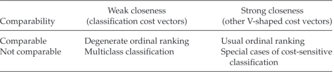
Table 1: Properties of Different Learning Problems.

Weak closeness Strong closeness

Comparability (classification cost vectors) (other V-shaped cost vectors) Comparable Degenerate ordinal ranking Usual ordinal ranking Not comparable Multiclass classification Special cases of cost-sensitive

classification

three-star one, which is in turn “worse than” a four-star one; movies of less than three stars are “worse than” movies of at least three stars.

The simplicity of the grouping and the comparison distinguishes or-dinal ranking from multiclass classification. For instance, when classify-ing movies, it is difficult to group {action movies,romantic movies_} and compare with {comic movies, thriller movies}, but “movies of less than three stars” can be naturally compared with “movies of at least three stars.”

The comparability property connects ordinal ranking to monotonic clas-sification (Sill, 1998; Kotl!owski & Sl!owi ´nski, 2009), which is also referred to as ordinal classification with the monotonicity constraints and is an im-portant problem on its own. Monotonic classification models the ordinal ranking problem by assuming that an explicit order in the input space (such as the value-order of one particular feature) can be used to directly (and monotonically) infer about the order of the ranks in the output space (y≤y-_{). In other words, monotonic classification allows putting thresholds} on the explicit order to perform ordinal ranking. The comparability prop-erty shows that there is an order (total preorder) introduced by the ranks. Nevertheless, the order is not always explicit in general ordinal ranking problems. Therefore, many of the existing ordinal ranking approaches, such as the thresholded model, which is discussed in section 5, seek the implicit order through transforming the input vectors before respecting the monotonic nature between the implicit order and the order of the ranks.

In Table 1, we summarize four different learning problems in terms of their comparability and closeness properties. As discussed, usual ordinal ranking problems come with strong closeness inY (which is represented by V-shaped cost vectors) and simple comparability inX. The classification cost vectors can be viewed as degenerate V-shaped cost vectors, and hence introduce degenerate ordinal ranking problems.

Multiclass classification problems, on the other hand, do not allow exam-ples of different classes to be naturally grouped and compared. If we want to use cost vectors other than the classification ones, we move to special cases of cost-sensitive classification. For instance, in the attempt to recog-nize digits{0,1, . . . ,9_}for written checks, a possible cost is the absolute one (to represent monetary differences) rather than simply right or wrong (the

classification cost). The absolute cost is V-shaped and convex. Nevertheless, the digits intuitively cannot be grouped and compared, and hence the recognition problem belongs to cost-sensitive multiclass classification rather than ordinal ranking (Lin, 2008).

A good ordinal ranking algorithm should appropriately use the compa-rability property. In section 4, we show how the property serves as a key to derive our proposed reduction framework.

3 Related Literature

The analysis of ordinal data has been studied in statistics by defining a suitable link function that models the underlying probability for generat-ing the ordinal labels (Anderson, 1984). For instance, one popular model is the the cumulative link model (Agresti, 2002), which we discuss in sec-tion 5. Similar models can be traced back to the work of McCullagh (1980). Much of the earlier work in statistics, which usually focuses on the effec-tiveness and efficiency of the modeling, influences ordinal ranking stud-ies in machine learning (Herbrich et al., 2000), including our work. An-other related area that studies the analysis of ordinal data is operations research, especially in the subarea of multicriteria decision analysis (Greco, Sl!owi ´nski, & Matarazzo, 2000; Figueira, Greco, & Ehrgott, 2005), which contains work that focuses on reasonable decision making with ordinal preference scales. Our work tackles ordinal ranking problems from the machine learning perspective—improving the test performance—and is different from work that takes the perspective of statistics or operations research.

In machine learning (and information retrieval), there are three ma-jor families of ranking algorithms: pointwise, pairwise, and listwise (Liu, 2009). The ordinal ranking setup presented in section 2 belongs to point-wise ranking. Next, we discuss some representative algorithms in each family and relate them to the ordinal ranking setup. Then we compare the proposed reduction framework with other reduction-based approaches for ranking.

3.1 Families of Ranking Algorithms

3.1.1 Pointwise Ranking. Pointwise ranking aims at predicting the rel-evance of some input vector x using either real-valued scores or ordinal-valued ranks. It does not directly use the comparison nature of ranking.

The ordinal ranking algorithms studied in this letter focus on comput-ing ordinal-valued ranks for pointwise rankcomput-ing. For obtaincomput-ing real-valued scores, a fundamental tool is traditional least-squares regression (Hastie, Tibshirani, & Friedman, 2001). As discussed in section 2, however, when the examples come with ordinal labels, the ordinal ranking algorithms

studied in this letter can be more useful than traditional regression by taking the metricless nature of labels into account.

3.1.2 Pairwise Ranking. Pairwise ranking aims at predicting the rela-tive order between two input vectorsx andx- _{and thus captures the local} comparison nature of ranking. It is arguably one of the most widely used techniques in the ranking family and is usually cast as a binary classifica-tion problem of predicting whetherxis preferred overx-_{. During training,} such a problem translates to comparing all pairs of (x_n,x_m)based on their corresponding labels. One representative pairwise ranking algorithm is RankSVM (Herbrich et al., 2000), which trains an underlying support vec-tor machine using those pairs. RankSVM was initially proposed for data sets that come with ordinal labels, but is also commonly applied to data sets that come with real-valued labels.

Note that even when all the labels take ordinal values, as long as two of the classes contain!(N)examples, there are!(N2_{)pairs. Such a quadratic} number of pairs makes it difficult to scale up general pairwise ranking algorithms, except in special cases like the linear support vector machine (Joachims, 2006) or RankBoost (Herbrich et al., 2000; Lin & Li, 2006). Thus, when the training set is large and contains ordinal labels, the ordinal ranking algorithms studied in this letter may serve as a useful alternative over pairwise ranking ones.

3.1.3 Listwise Ranking. Listwise ranking aims at ordering a whole finite set of input vectors S- = {x

-m}Mm=1. In particular, the (listwise) ranker tries to minimize the inconsistency between the predicted permutation and the ground-truth permutation of S- (Liu, 2009). Listwise ranking captures the global comparison nature of ranking. One representative listwise ranking algorithm is ListNet (Cao, Qin, Liu, Tsai, & Li, 2007), which is based on an underlying neural network model along with an estimated distribution of all possible permutations (rankers). Nevertheless, there areM! permu-tations for a given_S-_{. Thus, listwise ranking can be computationally even} more expensive than pairwise ranking.

Many listwise ranking algorithms try to alleviate the computational bur-den by keeping some internal pointwise rankers. For instance, ListNet uses the underlying neural network to score each instance (Cao et al., 2007) for the purpose of permutation. The use of internal pointwise rankers for listwise ranking further justifies the importance of better understanding pointwise ranking, including the ordinal ranking algorithms studied in this letter.

3.2 Reduction Approaches for Ranking. Because ranking is a relatively new and diverse problem in machine learning, many existing ranking ap-proaches try to reduce the ranking problem to other learning problems. Next, we discuss some existing reduction-based approaches that are re-lated to the framework proposed in this letter.

3.2.1 From Pairwise Ranking to Binary Classification. Balcan et al. (2007) propose a robust reduction from bipartite (i.e., ordinal with two outcomes) pairwise ranking to binary classification. The training part of the reduction works like usual pairwise ranking: learning a binary classifier on whetherx is preferred overx-_{. The prediction part of the reduction asks the underlying} binary classifier to vote for each example in the test set in order to rank those examples. The reduction is simple but yields solid theoretical guarantees. In particular, for ranking Mtest examples, the reduction uses !(M2_)calls to the binary classifier and transforms a binary classification regret of rto a bipartite ranking regret (measured by the so-called AUC criterion) of at most 2r.

Ailon and Mohri (2008) improve the reduction of Balcan et al. (2007) and propose a more efficient reduction from general pairwise ranking to binary classification. The prediction part of the reduction operates by taking the underlying binary classifier as the comparison function of the popular QuickSort algorithm. In the special bipartite ranking case, for ranking M examples, the reduction uses O(MlogM) calls to the binary classifier in average and transforms a binary classification regret of r to a bipartite ranking regret of at most 2r.

3.2.2 From Listwise Ranking to Regression (Pointwise Ranking). The subset ranking (Cossock & Zhang, 2008) algorithm can be viewed as a reduction from listwise ranking to regression. In particular, Cossock and Zhang (2008) prove that regression with various cost functions can be used to approxi-mate a Bayes optimal listwise ranker. In other words, low-regret regressors can be cast as low-regret listwise rankers.

3.2.3 From Listwise Ranking to Ordinal (Pointwise) Ranking. McRank (Li, Burges, & Wu, 2008) is a reduction from listwise ranking to ordinal rank-ing with the classification cost. The main theoretical justification of the reduction shows that a scaled classification cost of an ordinal ranker can upper-bound the regret of the associated listwise ranker. That is, low-error ordinal rankers can be cast as low-regret listwise rankers. Li et al. (2008) em-pirically verified that McRank can perform better than the subset ranking algorithm (Cossock & Zhang, 2008).

3.2.4 From Ordinal Ranking to Binary Classification. The proposed frame-work in this letter and in the associated shorter version (Li & Lin, 2007b) is a reduction from ordinal ranking to binary classification. We will show that the reduction is both error and regret preserving. That is, low-error binary classifiers can be cast as low-error ordinal rankers; low-regret binary classifiers can be cast as low-regret ordinal rankers.

The data replication method, which was independently proposed by Cardoso and da Costa (2007), is a similar but more restricted case of the reduction framework. The data replication method essentially considers

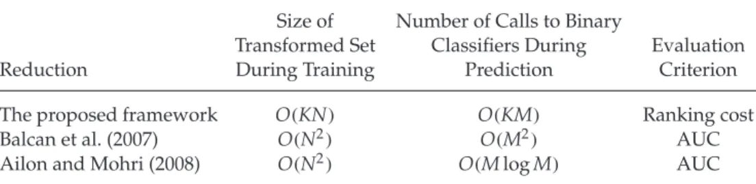
Table 2: Comparison of General Reductions from Ranking to Binary Clas-sification. Reduction Size of Transformed Set During Training

Number of Calls to Binary Classifiers During

Prediction

Evaluation Criterion

The proposed framework O(KN) O(KM) Ranking cost

Balcan et al. (2007) O(N2_{) O(M}2_{) AUC}

Ailon and Mohri (2008) O(N2_{) O(MlogM) AUC}

the absolute cost. In addition, the focus of the data replication method (Cardoso & da Costa, 2007) is on explaining the training procedure of the reduction. The proposed framework in this letter is more general than the data replication method in terms of the cost considered, as well as the deeper theoretical analysis on both the training and the test performance of the reduction.

The proposed reduction framework for pointwise ranking and existing reductions in pairwise ranking (Balcan et al., 2007; Ailon & Mohri, 2008) take very different views on the ranking problem and considers different eval-uation criteria. As a consequence, when learningNexamples and ranking (predicting on)Minstances withKordinal scales, the proposed framework results in a transformed training set of sizeO(KN) and a prediction pro-cedure with time complexityO(KM). Both the size of the training set and the time complexity of the prediction procedure are more efficient than the state-of-the-art reduction from pairwise ranking to binary classification (Ailon & Mohri, 2008), as shown in Table 2.

Note that the work of Li et al. (2008) revealed an opportunity to use the discrete nature of ordinal-valued labels to improve the listwise ranking performance over subset ranking when using a heuristic ordinal ranking algorithm. The proposed framework is a more rigorous study on ordinal ranking that can be coupled with McRank to yield a reduction from listwise ranking to binary classification, which allows state-of-the-art binary classifi-cation algorithms to be efficiently used for listwise ranking. We demonstrate the use of this opportunity in section 6.4.

4 Reduction Framework

We first introduce the details of our proposed reduction framework. Then we demonstrate its theoretical guarantees. Consider, for instance, that we want to know how good a moviexis. Using the comparability property of ordinal ranking, we can then ask the associated question, “Is the rank ofx greater thank?”

For a givenk, such a question is exactly a binary classification problem, and the rank ofxcan be determined by asking multiple questions fork =1, 2, until(K−1). The questions are the core of the dominance-based rough set approach in operations research for reasoning from ordinal data (Sl!owi ´nski, Greco, & Matarazzo, 2007). From the machine learning perspective, Frank and Hall (2001) proposed to solve each binary classification problem in-dependently and combine the binary outputs to a rank. Although their approach is simple, the generalization performance using the combination step cannot be easily analyzed.

The proposed reduction framework works differently. First, a simpler step is used to convert the binary outputs to a rank, and generalization analysis can immediately follow. Moreover, all the binary classification problems are solved jointly to obtain a single binary classifier.

Assume thatg(x,k)is the single binary classifier that provides answers to all the associated questions above. Consistent answers would beg(x,k)₌

+1 (“yes”) for k=1 until ("₋1) for some ", and ₋1 (“no”) afterward. Then a reasonable ranker based on the binary answers is r_g(x)₌"₌1₊ min_{k:g(x,k)_{= +}1_}. Equivalently, r_g(x)_≡1₊ K−1 " k=1 [[g(x,k) >0]]. (4.1)

The binary classifier g that produces only consistent answers would be calledrank-monotonic.3

For any ordinal example (x,y,c), we can define the extended binary examples(X(k),Y(k))with weightsW(k)as

X(k)

=(x,k), Y(k) ₌2[[k <y]]₋1, W(k) ₌(K₋1)_{· |}c[k]₋c[k₊1]_| (4.2) The extended input vector X(k) _{represents the associated question, “Is the} rank ofxgreater thank?” The binary labelY(k)_{represents the desired answer} to the question; the weightW(k) _{represents the importance of the question} and will be used in our theoretical analysis. Here X(k) _{stands for an} ab-stract pair, and we discuss its practical encoding in section 5. If g(X(k)_)≡ g(x,k) makes no errors on all the associated questions, r_g(x) equals y by

3_{Although equation 4.1 can be flexibly applied even whengis not rank monotonic, a}

equation 4.1. That is, c[r_g(x)]₌0. In the following theorem, we further connectc[r_g(x)] to the amount of error thatgmakes.

Theorem 1 (per example cost bound). For any ordinal example(x,y,c), wherec is V-shaped and c[y]=0, consider its associated extended binary examples (X(k),Y(k),W(k))in equation 4.2. Assume that the ranker r_gis constructed from a binary classifier g using equation 4.1. If g(X(k))is rank-monotonic or ifcis convex, then c[r_g(x)]_≤ 1 K−1 K−1 " k=1 W(k)·##Y(k) +=g(X(k))$$. (4.3) Proof. Becausegis rank-monotonic,g(X(k)_{)= +1 fork <r}

g(x)andg(X(k))=

−1 fork≥r_g(x). Thus, the cost that the rankerr_gneeds to pay is c[r_g(x)]₌ K−1 " k=r_g(x) (c[k]₋c[k₊1])₊c[k] = K−1 " k=1 (c[k]₋c[k₊1])[[g(X(k)) <0]]₊c[k]. (4.4)

Because the cost vectorcis V-shaped,Y(k)_{equals the sign of(c[k]−c[k+1])} if the latter is not zero. Continuing from equation 4.4 withc[y]=0,

(K−1)_·c[r_g(x)] = y−1 " k=1 W(k)_·Y(k)_·[[g(X(k)_{) <0]]+(K−1)·c[k],} K−1 " k=y W(k)_·Y(k)_·(1−[[g(X(k)_{) >0]]),} = y−1 " k=1 W(k) ·[[Y(k)+=g(X(k))]]₊(k₋1)_·c[y]₊ K−1 " k=y W(k) ·[[Y(k) +=g(X(k))]] = K−1 " k=1 W(k)_·[[Y(k)_+=g(X(k)_{)]]. (4.5)} Whengis not rank-monotonic but the cost vectorcis convex, equation 4.5 becomes an inequality that could be alternatively proved by replacing

equation 4.4 with K−1 " k=r_g(x) (c[k]₋c[k₊1])_≤ K−1 " k=1 (c[k]₋c[k₊1])##g(X(k)) <0$$.

The inequality above holds because (c[k]₋c[k₊1]) is decreasing due to the convexity, and there are exactly (r_g(x)₋1)zeros and (K₋r_g(x)) ones in the values of [[g(X(k)_{) <0]] according to equation 4.1.}

We call equation 4.3 the per example cost bound, which says that if g makes only a small amount of error on the extended binary examples (X(k),Y(k),W(k)), thenr_gis guaranteed to pay only a small amount of the cost on the original example(x,y,c). The bound allows us to derive the follow-ing reduction method, which is composed of three stages: preprocessfollow-ing, training, and prediction.

Algorithm 1:Reduction to Extended Binary Classification

1. Preprocessing: For each original training example(x_n,y_n,c_n)_∈Sand for each k =1,2, . . . ,K₋1, generate an extended training example (X_n(k),Y_n(k),W_n(k))and include it in_SE, where

X(k)

n =(xn,k),Yn(k) =2[[k<yn]]−1, W(k)

n =(K−1)· |c[n][k]−c[n][k+1]|.

2. Training: Use a binary classification algorithm onSE and get a binary classifier g on a concrete encoding (discussed in section 5) of X ×

1,2, . . . ,K₋1. Letg(x,k)_≡g(X(k)).

3. Prediction: For anyx∈X, estimate its rank with equation 4.1.

4.1 Cost Bound of the Reduction Framework. Consider the follow-ing probability distribution_Pb(X(k),Y(k),W(k))that generates the extended binary examples:

1. Draw a tuple(x,y,c)independently from_P(x,y,c), and drawk uni-formly from the set 1,2, . . . ,K₋1.

2. Generate%X(k)_,Y(k)_,W(k)&_{by equation 4.2.}

The extended training setS_Econtains examples that are equivalent (in terms of expectation) to examples drawn independently fromPb(X(k),Y(k),W(k)). For any given binary classifierg, define its out-of-sample error with respect to_Pbas

Using the definitions above, we can prove the first theoretical guarantee of the reduction framework.

Theorem 2 (cost bound of the reduction framework). Consider a ranker r_g that is constructed from a binary classifier g using equation 4.1. Assume that c is V-shaped andc[y]=0for every tuple(x,y,c)generated from_P(c_|x,y). If g(x,k) is rank-monotonic or if every cost vectorcis convex, then E(r_g)_≤E_b(g).

Proof. From equation 4.3,

c[r_g(x)]_≤ 1 K₋1 K−1 " k=1 W(k)·##Y(k) +=g(X(k)₎$$_.

Take the expectation overP on both sides and use∼uto mean the uniform sampling: E(r_g)_{≤ E} (x,y,c)∼P 1 K−1 K−1 " k=1 W(k)_·##_Y(k) _+=g(X(k)₎$$ = E (x,y,c)∼P k∼u{1,...,KE −1} W(k)_·##_Y(k) _+=g(X(k)₎$$ = E (X,Y,W)∼Pb W_·[[Y ₊₌g(X)]] =E_b(g).

4.2 Regret Bound of the Reduction Framework. Theorem 2 indicates that if there exists a decent binary classifier g, we can obtain a decent ranker r_g. Nevertheless, it does not guarantee how good r_g is in compar-ison with other rankers. In particular, if we consider the optimal binary classifierg_∗underP[b](X,Y,W), and the optimal rankerr∗ underP(x,y,c), does a small regretE_b(g)−E_b(g_∗)in binary classification translate to a small regretE(r_g)₋E(r_∗)in ordinal ranking? Furthermore, isE(r_g

∗)close toE(r∗)?

Next, we introduce the reverse-reduction technique, which helps to answer these questions.

The reverse-reduction technique works on the binary classification prob-lems generated by the reduction method. It goes through the preprocessing and the prediction stages of the reduction method in the opposite direc-tion. In the preprocessing stage, instead of starting with ordinal exam-ples (x_n,y_n,c_n), reverse reduction deals with weighted binary examples (X_n(k),Y_n(k),W_n(k)). It first combines each set of binary examples sharing the

samex_nto an ordinal example by              y_n=1+ K−1 " k=1 ## Y_n(k) >0$$_; c_n[k]₌ K−1 " "=1 W(") n K−1 ·[[yn≤" <kork < "≤yn]]. (4.6)

It is easy to verify that equation 4.6 is the exact inverse transform of equation 4.2 on the training examples under the assumption that c[y]=0. These ordinal examples are then given to an ordinal ranking algorithm to obtain a rankerr. In the prediction stage, reverse reduction works by decomposing the prediction r(x) to K₋1 binary predictions, each as if coming from a binary classifier:

g_r(X(k))₌2[[r(x) >k]]₋1. (4.7)

Then a lemma on the out-of-sample cost ofg_r immediately follows (Lin & Li, 2009).

Lemma 1. With the definitions of P(x,y,c) and _Pb(X(k),Y(k),W(k)) in theorem 2, for every ordinal ranker r, E(r)=E_b(g_r).

Proof. Becauseg_r is rank-monotonic by construction, the same proof for the first part of theorem 2 leads to the desired result.

The stages of reduction and reverse reduction are illustrated in Figure 1. Next, we show how the reverse-reduction technique allows us to draw a strong theoretical connection between ordinal ranking and binary classification. By the definition ofr_∗andg_∗, for any rankerrand any binary classifierg,

E(r)≥E(r_∗), E_b(g)_≥E_b(g_∗). (4.8) Then the reverse-reduction technique yields a simple proof of the regret bound.

Theorem 3 (regret bound of the reduction framework). If g(x,k)is rank-monotonic or if every cost vectorcis convex, then

Figur e 1: Reduction (top) and reverse reduction (bottom).

Proof.

E(r_g)₋E(r_∗)_≤E_b(g)₋E(r_∗) (from theorem 2)

=E_b(g)−E_b(g_r

∗) (from lemma 1) ≤E_b(g)−E_b(g_∗) (from equation 4.8).

The cost bound (theorem 2) and the regret bound (theorem 3) provide different guarantees for the reduction method. The former describes how the ordinal ranking cost is upper-bounded by the binary classification error in an absolute sense, and the latter describes the upper bound in a relative sense.

4.3 Equivalence Between Ordinal Ranking and Binary Classification. The results thus for suggest that ordinal ranking can be reduced to binary classification without any loss of optimality. That is, ordinal ranking is no harder than binary classification. Intuitively, binary classification is also no harder than ordinal ranking, because the former is a special case of the latter withK=2. Next, we formalize the notion of hardness with the probably ap-proximately correct (PAC) setup in computational learning theory (Kearns & Vazirani, 1994) and prove that ordinal ranking and binary classification are indeed equivalent in hardness. We use the following definition of PAC in our upcoming theorems (Valiant, 1984; Kearns & Vazirani, 1994).

Definition 1. In cost-sensitive classification, a learning model G is efficiently PAC-learnable (using the same representation class) if there exists a (possibly randomized) learning algorithm A satisfying the following property: for every distributionP(x,y,c)being considered, where

c[g_∗(x)]₌c[y]₌c_{min =}0,

with some g_∗ ∈G; for all 0< # and 0< δ < 1₂, if _Ais given access to an oracle generating examples (x,y,c) from _P(x,y,c), as well as inputs# and δ, then_A outputs g∈G such that E(g)≤# with probability at least1₋δ, as well as with time polynomial in 1

# and 1 δ.

The definition assumes that the target functiong_∗ is within the learning model _G and is of cost 0 (the minimum cost). In other words, it is the noiseless setup of learning. We shall focus on only this case while pointing out that similar results can also be proved for the noisy setup (Lin, 2008). Theorem 4 (equivalence theorem of the reduction framework). Consider a learning model Rfor ordinal ranking, its associated learning model G= {g_r:r∈R} for binary classification, and distributionsP(x,y,c) such that all cost vectors c are

V-shaped. ThenRis efficiently PAC-learnable if and only ifG is efficiently PAC-learnable.

Proof. If G is efficiently PAC-learnable using algorithm A_G, we can convertA_Gto an efficient algorithmA_Rfor ordinal ranking as follows:

1. Transform the oracle that generates(x,y,c)from_P(x,y,c)to an oracle that generates(X(k),Y(k),W(k))by picking kuniformly and applying equation 4.2.

2. RunA_Gwith the transformed oracle until it outputs someg(X(k)). 3. Returnr_g.

It is not hard to see that A_R is as efficient asA_G, and the cost guarantee comes from theorem 2 using the fact thatg_rare all rank-monotonic.

Now we consider the other direction. If Ris efficiently PAC-learnable using algorithm A_R, we can convert A_R to an efficient algorithm A_G for binary classification:

1. Transform the oracle that generates (X(k),Y(k),W(k)) from Pb(X(k),Y(k),W(k))to an oracle that generates(x,y,c)by

x₌(X(k)[1],X(k)[2], . . . ,X(k)[D])_; c=              W(k) K−1 ·(0+ ,- ., . . . ,0 k ,1, . . . ,1) forY(k) _{= −}1, W(k) K−1 ·(1+ ,- ., . . . ,1 k ,0, . . . ,0) forY(k) _{= +}1_; y=argmin 1≤"≤K

c["], with ties arbitrarily broken.

That is,x copies the 1st to theDth elements of X(k)_{. Let P˜(x,y,c)be} the underlying distribution of the constructed oracle.

2. RunA_Rwith the transformed oracle until it outputs somer(x). 3. Returng_r.

Note that_AGis as efficient as_AR. In addition, we see that plugging_P˜ into equation 4.2 introducesPb. Thus, if we takeE(r)˜ as the expected test cost with respect to_P˜, by lemma 1,

E_b(g_r)_{= ˜}E(r)for allr_∈R.

Therefore,E_b(g_r) < #after running_AG.

Theorem 4 demonstrates that ordinal ranking is theoretically as easy (hard) as the associated binary classification problem. Recall that we com-pare four different kinds of learning problems in Table 1. At first sight,

theorem 4 appears to suggest that all four problems can be conquered with the reduction framework, because the only required assumption of the theorem is that the cost vectors are V-shaped. Nevertheless, note that the necessary and sufficient condition in the theorem is, “The associated learn-ing modelGis efficiently PAC-learnable.” Then the different comparability properties of the different problems make a difference. In particular, for multiclass classification problems, the associated binary question, “Is the class ofxgreater thank?” can be complicated and is thus difficult to learn, In other words, the associatedGmay not be efficiently PAC-learnable. Then more complicated binary questions (Abe et al., 2004; Beygelzimer, Daniand, Hayes, Langford, & Zadrozny, 2005; Beygelzimer, Langford, & Ravikumar, 2007; Lin, 2008) are needed to reduce from the general (cost-sensitive) mul-ticlass problem to binary classification ones.

On the other hand, for the special case of cost-sensitive ordinal ranking, in which_Gis efficiently PAC-learnable, the reduction framework establishes a tight connection between the learnability ofGandR—the ranking model of interest. The tight connection motivates us to design ordinal ranking algorithms from popular binary classification algorithms, as we show in the next section.

5 Applications of Reduction Framework

So far the reduction works only by assuming thatX(k) _{=(x,k)is an abstract} pair understandable by the binary classification algorithm. With proper choices of the cost vectors, the encoding scheme of (x,k), and the binary classification algorithm, many existing ordinal ranking algorithms can be unified in our framework, and their theoretical justifications can immedi-ately follow.

In this section, we briefly discuss some of those algorithms and their theoretical justifications. It happens that a simple encoding scheme for(x,k) via a coding matrix M of (K−1) rows works for all the algorithms. To formX(k)_{, the vectorm}

k, which denotes thekth row ofM, is appended after x. We mostly work withM=γ _·I_K−1, whereγ is a positive scalar andI_K−1 is the(K−1)_×(K₋1)identity matrix.

5.1 Perceptron for Ordinal Ranking. The perceptron ranking (PRank) algorithm proposed by Crammer and Singer (2005) is an online ordinal ranking algorithm that employs the thresholded linear model,

r(x)₌min_{k:₀v,x_{1 ≤}θ_k},

where the thresholds θ₁, θ₂, . . . , θ_K−1, θ_K are ordered such that θ_1≤θ_2≤

· · · ≤θ_K−1≤θ_{K= ∞}. Whenever a training example is not predicted cor-rectly, the currentv and θ are updated in a way similar to the perceptron

learning rule (Rosenblatt, 1962). The algorithm was proved to keep the thresholds ordered along with a mistake bound (Crammer & Singer, 2005).

LetX(k) _=(x,m

k)with the simple encoding schemeM=IK−1. Then, r(x)₌min_{k:₀v,x_{1 ≤}θ_{k} =}1₊

K−1 " k=1

[[0(v,₋θ),X(k)₁>0]].

Consider an ordinal ranking problem such that_P(x,y,c)only generates ex-amples(x,y,c(y)), wherec(y)is the absolute cost vector with respect toy. We see thatW(k) _{=K−1 (a constant) for all the extended binary examples. Then} we can simply interpret PRank as a specific instance of the reduction frame-work with a modified perceptron learning rule as the underlying binary classification algorithm. That is, PRank uses the perceptron learning rule to find a weight vector (v,₋θ) for classifying the extended binary examples (x,m_k).4The mistake bound is a direct application of the well-known per-ceptron mistake bound (see Freund & Schapire, 1999). Our framework not only simplifies the derivation of the mistake bound, but also allows the use of other underlying perceptron algorithms, such as batch-mode algorithms (Li & Lin, 2007a) rather than online ones.

5.2 Boosting for Ordinal Ranking. In our earlier work (Lin & Li, 2006), we proposed the thresholded ensemble model

r(x)₌min_{k:H_T(x)_≤θ_k}, whereH_T(x)₌ T "

t=1

α_th_t(x), (5.1)

for ordinal ranking. Each confidence function h_t :_{X →}[₋1,₊1] reflects a possibly imperfect ordering preference. Note that a special instance of the confidence function is a binary classifier X → {−1,₊1_}. The ensemble linearly combines the ordering preferences withα. We allowα_t to be any real value, which means that it is possible to reverse the ordering preference ofh_tin the ensemble when necessary.

Ensemble models in general have been successfully used for classifica-tion and regression (Meir & R¨atsch, 2003). They not only introduce more sta-ble predictions through the linear combination, but also provide sufficient power for approximating complicated target functions. The thresholded ensemble model extends existing ensemble models to ordinal ranking and inherits many useful theoretical properties from them. Next, we discuss one such property: large-margin bounds.

4_{To precisely replicate the PRank algorithm, the (K−1)binary examples sprouted}

from a same ordinal example should be considered altogether in updating the perceptron weight vector.

We first list the definition of the margins for a thresholded ensemble (Lin & Li, 2006). Intuitively, we expect the potential value H_T(x) to be in the desired interval(θ_y−1, θ_y), and we wantH_T(x)to be far from the thresholds. Definition 2. Consider a given thresholded ensemble r in equation 5.1. The nor-malized marginρˆ_k(x,y)is defined as

ˆ ρ_k(x,y)₌(2[[k <y]]₋1)(H_T(x)₋θ_k) / 0_"T t=1 |α_{t| +} K−1 " k=1 |θ_k| 1 .

Definition 2 is similar to the definition of the support vector machine (SVM) margin made by Shashua and Levin (2003) and is analogous to the definition of the"₁-margins in binary classification (Schapire, Freund, Bartlett, & Lee, 1998). A nonpositive ρˆ_k(x,y)indicates an incorrect predic-tion. We now define the)-absolute margin cost as

E_in(r, ))_≡ 1 N N " n=1 K−1 " k=1 [[ρ_ˆk(x_n,y_n)_≤)]].

Consider an ordinal ranking problem such that_P(x,y,c)generates ex-amples only with the absolute cost vectors. The associated binary classifica-tion problem would then be based on an underlying probability distribuclassifica-tion P[b](X,Y,W)that generates onlyW =K−1 (a constant value). Then we can obtain a large-margin bound ofE(r):

Theorem 5 (large-margin bound for thresholded ensemble rankers). Consider a negation complete5_{setH, which contains only binary classifiers h:X → {−1,+1}} and is of VC-dimension d. Assume that δ >0, and N>d₊K₋1₌d_E. Then, for an ordinal ranking problem with the absolute cost vectors, with probability at least 1−δover the random choice of the training set S, every thresholded ensemble ranker defined from equation 5.1 satisfies the following bound for all) >0:

E(r)_≤E_in(r, ))₊O  _√K N 0 d_Elog2(N/d_E) )2 +log 1 δ 11/2 . Proof. See appendix A.

The bound above can be generalized whenHcontains confidence func-tions rather than binary classifiers using another existing result (Schapire et al., 1998, theorem 4) in the proof. The bound motivates us to design the

5_{His negation complete if and only ifh∈H⇐⇒(−h)∈H, where(−h)(x)= −(h(x))}

ORBoost-All algorithm (Lin & Li, 2006), which can be viewed as coupling the reduction framework with a variant of the popular AdaBoost algorithm (Schapire et al., 1998; Schapire & Singer, 1999). ORBoost-All provably mini-mizes the termE_in(r, ))exponentially fast if the underlying base learner is strong enough. The proof can be made by applying the training error theo-rem of AdaBoost (Schapire et al., 1998, theotheo-rem 5) onS_E, another application of the reduction framework.

5.3 SVM for Ordinal Ranking. SVM is a popular binary classification algorithm (Vapnik, 1995; Sch¨olkopf & Smola, 2002). It maps the feature vec-torxtoφ(x)in a possibly higher-dimensional space and implicitly computes the inner products with a kernel functionK(x,x-)_{= 0}φ(x), φ(x-)₁.

Using a similar set of notations for perceptions (see section 5.1), we denote the parallel hyperplanes in the higher-dimensional space by(v,₋θ) with an additional bias term b. Now, if we encode (x,k) with the matrix M=γ _·I_K−1, we can then compute the inner products of the extended examples(X(k),Y(k))by

KE((x,k), (x-,k-))= 0(φ(x), γ1k), (φ(x-), γ1k-)-1=K(x,x-)+γ2[[k=k-]].

With the reduction framework, we can plug in KE and O %

NK& extended training examples into the standard SVM to obtain a hyperplane ranker,

r(x)₌1₊ K−1 " k=1

[[0v, φ(x)_{1 +}b₋θ_k >0]], based on an optimal solution to

min v,b,θ_k,ξ(k) n 1 20v,v1 + 1 2γ20θ,θ1 +κ N " n=1 K−1 " k=1 W(k) n ξn(k), (5.2) subject to Y(k) n (0v, φ(x)1 +b−θk)≥1−ξn(k), ξ_n(k) _≥0, forn₌1, . . . ,N, and k₌1, . . . ,K₋1. If θ_{1 ≤}θ_{2 ≤ · · · ≤}θ_K−1 or if the cost vectors considered are convex, theorems 2 and 3 can guarantee the expected out-of-sample cost of r(x) based on the expected out-of-sample cost of the binary classifier:

g(x,k)₌sign(₀v, φ(x)_{1 +}b₋θ_k).

The oSVM approach of Cardoso and da Costa (2007) is an instance of equation 5.2 with the absolute cost vectors, in which all Wn(k) are equal. The SVOR-IMC approach of Chu & Keerthi (2007) can also be thought of as

a modified instance of the formulation with the absolute cost vectors, except that the _2γ12 0θ , θ1term is dropped. Their SVOR-EXC approach is another modified instance using the classification cost vectors plus an additional constraint to guarantee thatθ_{1 ≤}θ_{2 ≤ · · · ≤}θ_K−1.

Our proposed algorithm, reduction-to-SVM (RED-SVM) unifies the above algorithms under a generic formulation, equation 5.2, with the cost-sensitive reduction framework. RED-SVM can deal with any convex cost vectors by changingWn(k) and feeding the weighted binary examples to a standard SVM solver, regardless of whetherθ_1≤θ_{2≤ · · · ≤}θ_K−1. Interest-ingly, our earlier work (Li & Lin, 2007b) proved that the ordering property always holds at the optimal SVM solution.

On the other hand, if the cost vectors are ordinal but not convex, solving equation 5.2 is more complicated. We adopt a coordinate-descent procedure that switches between optimizing (v,b) (using the standard SVM solver) and optimizing θ under the constraints (a small quadratic programming

problem with an analytic solution) in the experiments.

Chu and Keerthi (2007) empirically found that SVOR-EXC performed better in terms of the classification cost, and SVOR-IMC preceded in terms of the absolute cost. They explain so by noting that SVOR-EXC minimizes an in-sample loss function that upper-bounds the classification cost, while SVOR-IMC minimizes a loss function that upper-bounds the absolute cost. The explanation is echoed by the study of loss functions for ordinal ranking (Rennie & Srebro, 2005; Dembczy ´nski et al., 2008). The proposed reduc-tion framework offers a more direct explanareduc-tion than the loss-based one. Because the binary SVM is designed to target for decent out-of-sample binary classification error, reduction with the classification cost (SVOR-EXC) targets for decent out-of-sample classification cost and reduction with the absolute cost (SVOR-IMC) targets for decent out-of-sample absolute cost.

Note that Chu and Keerthi (2007) spent a great deal of effort in designing and implementing suitable optimizers for the modified formulation that does not contain the 1

2γ2 0θ , θ1 term. If we use the standard soft-margin SVM instead when considering the convex cost vectors like the absolute cost, we can directly and efficiently use the state-of-the-art SVM software to deal with the ordinal ranking problem. The formulation of Chu and Keerthi (2007) can be approximated by using a largeγ. As we shall see in section 6, even a simple assignment ofγ ₌1 performs similarly to the approaches of Chu and Keerthi (2007) in practice.

In addition to the algorithmic benefits, the reduction framework can be used theoretically for SVM. For instance, we demonstrated how we can derive a novel large-margin absolute-cost bound of thresholded ensemble rankers in section 5.2. Next, we extend the bounds to SVM-based formula-tions and to a wider class of cost funcformula-tions. While Shashua and Levin (2003) derived one such bound with a specific cost function, their bound is not data dependent and hence does not fully explain the out-of-sample performance

of SVM-based rankers in reality (Bartlett & Shawe-Taylor, 1998). Our bound, on the other hand, is not only more general but also data dependent: Theorem 6 (large-margin bound for SVM-based rankers). Consider a collection

F= {f(x,k)_{= 0}v, φ(x)₁₊b₋θ_k :₄v₄2₊₄b₋θ₄2 _≤1,₄φ(x)₄2₊1_≤R2_}. Let B_max =max_c∈C(c[1]₊c[k]), B_{min =}min_c∈C(c[1]₊c[k]), and β ₌B_max/ B_min. If θ_1≤θ_{2 ≤ · · · ≤}θ_K−1, or if everyc is convex, for any ) >0, with prob-ability at least 1−δ, and for every f in F, the associated ranker rg(x) with g(·)₌sign(f(_·))satisfies E(r_g)_≤ β N·(K−1) N " n=1 K−1 " k=1 W(k) n ## Y(k) n f(X(k)n )≤) $$ +O 0 logN √ N , R ), 6 log1 δ 1 .

Proof. See appendix B.

Thus, if the binary classifier gachieves large margins (_≥)) on most of the extended training examples(X(k)_n ,Y_n(k),W_n(k)),E(r_g)is guaranteed to be small.

Theorem 6, which is based on the proposed reduction framework, is quite general and applies to a wide class of cost functions. In the special case of the absolute cost function (which results inWn(k) =1 andβ =1), theorem 6 can be simplified to an order-wise comparable bound that has been inde-pendently derived by Agarwal (2008) using a similar proving technique.

Note that we can also choose to encode (x,k) differently. For instance, define

¯

KE((x,k), (x-,k-))=[[k =k-]]0φk(x), φk(x-)1 =[[k=k-]]Kk(x,x-).

That is, different kernels can be used for different binary classification sub-problems. Recently Chang, Chen, and Hung (2011) explored such a possibility and proposed the ordinal hyperplanes ranker that achieved promising performance on the age-estimation application. The ordinal hyperplanes ranker can be theoretically justified through the reduction framework using the choice of encoding above. The promising performance suggests the possibility of application opportunities within the proposed general framework.

5.4 Summary. We have briefly introduced several ordinal ranking algorithms that can be explained as special instances of the reduction framework. We have also derived new cost bounds of the ordinal ranking

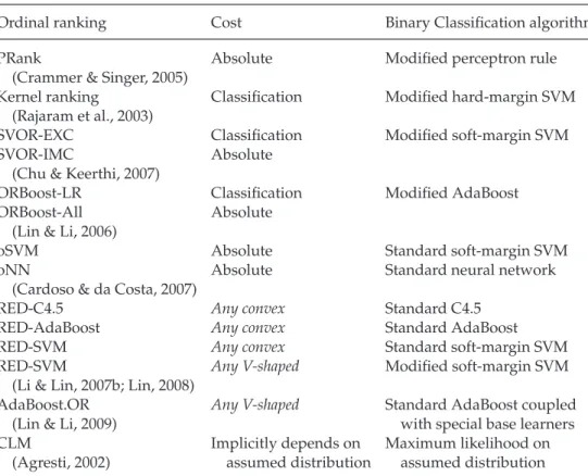
Table 3: Instances of the Reduction Framework.

Ordinal ranking Cost Binary Classification algorithm

PRank Absolute Modified perceptron rule

(Crammer & Singer, 2005)

Kernel ranking Classification Modified hard-margin SVM

(Rajaram et al., 2003)

SVOR-EXC Classification Modified soft-margin SVM

SVOR-IMC Absolute

(Chu & Keerthi, 2007)

ORBoost-LR Classification Modified AdaBoost

ORBoost-All Absolute

(Lin & Li, 2006)

oSVM Absolute Standard soft-margin SVM

oNN Absolute Standard neural network

(Cardoso & da Costa, 2007)

RED-C4.5 Any convex Standard C4.5

RED-AdaBoost Any convex Standard AdaBoost

RED-SVM Any convex Standard soft-margin SVM

RED-SVM Any V-shaped Modified soft-margin SVM

(Li & Lin, 2007b; Lin, 2008)

AdaBoost.OR Any V-shaped Standard AdaBoost coupled

(Lin & Li, 2009) with special base learners

CLM Implicitly depends on Maximum likelihood on

(Agresti, 2002) assumed distribution assumed distribution

algorithms via reduction. There are some other existing algorithms that can be viewed as special instances of the reduction framework, as listed in Table 3.

Note that the thresholded linear model is commonly used in statistics for ordinal ranking (Agresti, 2002) and is called the cumulative link model (CLM), which assumes %0v,x_{1 −}θ_k& to link to the cumulative probability P%y≥k|x&. CLM can then be coupled with some more assumptions on

the underlying probability distribution to reach a maximum likelihood solution. The proposed framework treats the thresholded linear model (CLM) as a rank-monotonic special case of the general prediction rule, equation 3.1. CLM and the proposed framework take very different views on modeling the ordinal ranking problem and hence reach different results. In particular, CLM focuses on deriving from the assumed underlying dis-tribution appropriately, while the proposed framework focuses on using the given cost vectors appropriately.

6 Experiments

We validate the proposed reduction framework by performing experiments with eight benchmark ordinal ranking data sets (Chu & Keerthi, 2007):

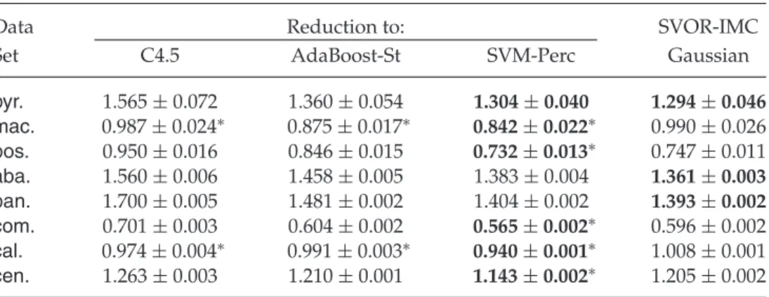
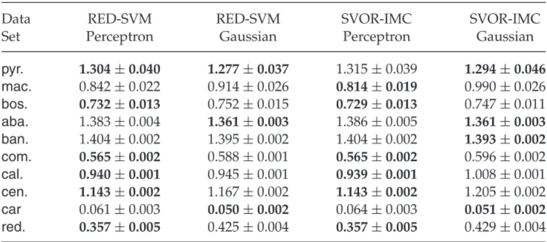
Table 4: Test Absolute Cost of Ordinal Ranking Algorithms.

Data Reduction to: SVOR-IMC

Set C4.5 AdaBoost-St SVM-Perc Gaussian

pyr. 1.565±0.072 1.360±0.054 1.304±0.040 1.294±0.046 mac. 0.987±0.024∗ _0.875±0.017∗ _0.842±0.022∗ _0.990±0.026 bos. 0.950±0.016 0.846±0.015 0.732±0.013∗ _0.747±0.011 aba. 1.560±0.006 1.458±0.005 1.383±0.004 1.361±0.003 ban. 1.700±0.005 1.481±0.002 1.404±0.002 1.393±0.002 com. 0.701±0.003 0.604±0.002 0.565±0.002∗ _0.596±0.002 cal. 0.974±0.004∗ _0.991±0.003∗ _0.940±0.001∗ _1.008±0.001 cen. 1.263±0.003 1.210±0.001 1.143±0.002∗ _1.205±0.002

Notes: Those within one standard error of the lowest one are marked in bold. Those better than SVOR-IMC are marked with an asterisk.

pyrimdines, machine, boston, abalone, bank, computer, california, census. The data sets were constructed by quantizing some metric regression data sets withK = 10. We use the same training-to-test ratio and also average the results over 20 trials. Thus, we can fairly compare our results with those of SVOR-IMC and SVOR-EXC (Chu & Keerthi, 2007), the state-of-the-art algorithms.

6.1 The Absolute Cost. We first test the reduction framework with the absolute cost vectors, M=γ _·I_K−1 withγ ₌1, and three different binary classification algorithms. The first binary algorithm is the C4.5 decision tree (Quinlan, 1986).6 _{The second is AdaBoost-St, which uses AdaBoost} (Schapire et al., 1998) to aggregate 500 decision stumps. The third one is SVM-Perc, which is SVM (Vapnik, 1995) with the perceptron kernel (Lin & Li, 2008). The parameter κ of the soft-margin SVM is determined by a five-fold cross-validation procedure with log₂κ _{∈ {−}17,₋15, . . . ,3_} (Hsu, Chang, & Lin, 2003), and LIBSVM (Chang & Lin, 2001) is adopted as the solver.

We list the mean and the standard error of the test absolute costs in Table 4, with entries within one standard error of the lowest one marked in bold.7 _{With the proposed reduction framework, all three binary} learn-ing algorithms, even the simplest C4.5 decision tree, could be better than SVOR-IMC with the gaussian kernel on some of the data sets. The re-sults demonstrate that all the algorithms can achieve decent out-of-sample

6_{C4.5 can directly take the extended input vector(x,k)without encoding. We choose}

to still encode(x,k)by the matrixM=γ ·I_K−1 to make a simple and fair comparison with the other two algorithms that need the encoding.

7_{Note that the results from Chu and Keerthi (2007) include the standard deviation;}