Valiant Load-Balancing
Computer Systems Laboratory, Stanford University, Stanford, CA 94305-9030, USA {rzhang, nickm}@stanford.edu
Abstract. Network operators would like their network to support cur-rent and future traffic matrices, even when links and routers fail. Not surprisingly, no backbone network can do this today: It is hard to ac-curately measure the current matrix, and harder still to predict future ones. Even if the matrices are known, how do we know a network will support them, particularly under failures? As a result, today’s networks are designed in a somewhat ad-hoc fashion, using rules-of-thumb and crude estimates of current and future traffic.
Previously we proposed the use of Valiant Load-balancing (VLB) for backbone design. It can guarantee 100% throughput toany traffic ma-trix, even under link and router failures. Our initial work was limited to homogeneous backbones in which routers had the same capacity. In this paper we extend our results in two ways: First, we show that the same qualities of service (guaranteed support of any traffic matrix with or without failure) can be achieved in a realistic heterogeneous back-bone network; and second, we show that VLB is optimal, in the sense that the capacity required by VLB is very close to the lower bound of total capacity needed by any architecture in order to support all traffic matrices.
1
Introduction
A network operator would like their backbone network to serve customers’ de-mands at all times. But most networks have grown in an ad-hoc fashion, which – when considering failures and maintenance that frequently change the network – makes it impractical to systematically provision links so they have the capacity to carry traffic both during normal operation and under failures. To compensate, network operators tend to grossly over-provision their networks (typically below 20% utilization), because it is hard to know where new customers will join, what new applications will become popular, and when links and routers will fail.
It would help if we knew the traffic matrices the network will have to carry throughout its lifetime. Though the usual practice is to measure the current demand, and then extrapolate it to the future, the approach does not work for many reasons.
H. de Meer and N. Bhatti (Eds.): IWQoS 2005, LNCS 3552, pp. 178–192, 2005. c
°IFIP International Federation for Information Processing 2005 Zhang-Shen
First, Internet traffic is hard to measure. The number of entries in a traffic matrix is roughly quadratic in the number of nodes, so it is usually impractical to obtain all the measurements directly. To estimate the traffic matrix from incomplete measurements, the best techniques today give errors of 20% or more [6] [9]. More importantly, the traffic demand fluctuates over time, and it is hard to determine when thepeakusage of the network is. In practice, the “peak” is determined in an ad-hoc manner – by inspection, or some rules-of-thumb.
Second, even if we could accurately measure the current traffic matrix, it is hard to extrapolate to the future. Typically, estimates are based on historic growth rates, and adjusted according to marketing forecasts. But it’s hard to predict future growth rates and what new applications will become popular. Even if the total growth rate is estimated correctly, the growth may not be uniform across the whole network, and the introduction of new applications may change traffic patterns. For example, peer-to-peer traffic has demonstrated how quickly usage patterns can change in the Internet. The widespread use of voice-over-IP and video-on-demand may change usage patterns again over the next few years. What’s more, the growth rate does not take into account large new customers which may bring new demands. So network design has always used a wrong estimate of the future traffic matrix, and the designed network cannot guarantee to support the actual demand. It’s therefore not surprising that operators so heavily over-provision their networks.
In summary, existing networks, which have evolved in an ad-hoc fashion, have unpredictable performance. With current design techniques, it is hard to design a network with throughput guarantees because it is impossible to obtain a good estimate of the future traffic matrix. Once built, a network may have to work with a range of traffic conditions, but it is unknown to network operators as to how to design a network for a wide range of traffic matrices.
We recently proposed Valiant Load Balancing (VLB) [10], so that backbone networks can be designed to give strong guarantees on the support for an ar-bitrary set of traffic matrices, even under failure, and operate at much higher utilization (and hence higher efficiency and lower cost) than today. We assume that each backbone node in the network, or Point-of-Presence (PoP), has con-strained capacity, such as the aggregate capacity of the access network it serves, and design a backbone network to guarantee 100% throughput forany traffic matrix.
The limitations of designing a network for a specific traffic matrix, and the necessity to design for a wide range of traffic matrices, have been realized by some researchers recently, and a few schemes have been proposed [1] [5] [10] [7]. Most of these schemes use some type of load-balancing.
The VLB architecture makes the job of estimating the future traffic much simpler. While obtaining a traffic matrix estimation is hard, it is easier to mea-sure, or estimate, the total amount of traffic entering (leaving) a backbone node from (to) its access network. When a new customer joins the network, we add their aggregate traffic rate to the node. When new locations are planned, the aggregate traffic demand for a new node can be estimated from the population
that the node serves. While still not trivial, it is a lot easier than estimating the traffic from every node to every other node.
The Valiant load-balancing architecture has simple and efficient fault toler-ance so that only a small fraction of extra capacity is required to guarantee service under a number of failures in the network. The failure recovery can be quick because no new paths need to be established on the fly.
In this paper, we extend the result of [10] to networks with arbitrary node capacities. We will focus on deriving the optimal capacity allocation in this net-work and leave fault tolerance for future net-work. The rest of the paper is organized as follows: Section 2 introduces the VLB architecture and the notation used in this paper; Section 3 derives the lower bound on the required capacity to sup-port all traffic matrices and two load-balancing schemes which achieve capacity requirements close to the lower bound; We then relate our work to others’ and conclude the paper.
2
Valiant Load-Balancing
The Valiant load-balancing architecture was first proposed by L. G. Valiant for processor interconnection networks [8], and has received recent interest for scalable routers with performance guarantees [2] [4]. Keslassy et al. proved that uniform Valiant load-balancing is the unique architecture which requires the minimum node capacity in interconnecting a set of identical nodes [3]. We applied the VLB architecture to designing a predictable Internet backbone which can guarantee throughput to all traffic matrices, and can tolerate a number of link and router failures with only a small amount of excess capacity [10]. We will re-introduce the architecture and re-state the relevant results here before extending it to the more general scenario in backbone network design.
2.1 Previous Results
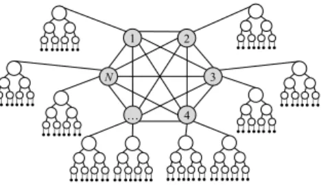
Consider a network consisting of multiple backbone nodes, or PoPs, intercon-nected by long-haul links. The network is arranged as a hierarchy, and each PoP
Fig. 1.A hierarchical network withN backbone nodes. The backbone nodes are con-nected by a (logical) full mesh, and each node serves an access network
1 2
3
N
connects an access network to the backbone (see Figure 1). For now, assume that there areN backbone nodes, and all of them are connected to access networks of the same aggregate capacity,r.
A full mesh of logical links of capacity 2r
N are established among theN
back-bone nodes. Traffic entering the backback-bone is load-balanced equally across allN
two-hop paths between ingress and egress. A packet is forwarded twice in the network: In the first stage, a node uniformly load-balances each of its incoming flows to all the N nodes, regardless of the packet destination. Load-balancing can be done packet-by-packet, or flow-by-flow at the application flow level. As-sume we can achieve perfect load-balancing, i.e., we can split traffic at the exact ratio we desire, then each node receives 1/N-th of every node’s traffic in the first stage. In the second stage, all packets are delivered to the final destination.
Uniform load-balancing leads to a guaranteed 100% throughput in this net-work. We consider the two packet forwarding stages. Since the incoming traffic rate to each node is at mostr, and the traffic is evenly load-balanced toNnodes, the actual traffic on each link due to the first stage routing is at most r
N. The
second stage is the dual of the first stage. Since each node can receive traffic at a maximum rate ofr, and it receives 1/N-th of the traffic from every node, the actual traffic on each link due to the second stage routing is also at most
r
N. Therefore, a full-mesh network where each link has capacity 2Nr is sufficient
to guarantee 100% throughput for any valid traffic matrix amongN nodes of access capacityr.
This is perhaps a surprising result – a network where each pair of nodes are connected with a link of capacity 2r
N can serve traffic matrices where a node can
send traffic to another node at rater. This shows the power of load-balancing. Valiant load-balancing makes sure that each flow is carried by N paths, and each link carries a fraction of many flows, therefore a large flow is evened out by other small flows. If all the traffic were to be sent through direct paths, we would need a full-mesh network of link capacity r. Therefore load-balancing is
N
2 times more efficient than direct routing. Although it may seem inefficient that
every packet should traverse the network twice, it has been proved that in order to serve all traffic matrices in a network of identical nodes, the uniform Valiant load-balancing architecture provides the unique optimal interconnection pattern which requires the lowest capacity at each node [3]. An even more surprising result is that the VLB network only requires a small fraction of extra capacity in order to tolerate failures in the network [10].
A common concern with load-balancing is that packets may incur a longer delay. In a Valiant load-balanced network, propagation delay is bounded by traversing twice the network diameter. Within the continental US, it’s been measured that this delay is well below 100ms, which is acceptable for all appli-cations we know of. We believe that VLB gives a reasonable tradeoff of increased fixed propagation delay for improved predictability, and lower delay variance.
In this paper, we consider Valiant load-balancing in a more general and more realistic case – we remove the assumption that all access networks have the same capacity. Once the backbone network is no longer symmetric, the first
stage load-balancing should no longer be uniform, and it is not clear what the optimal load-balancing scheme should be. In the rest of the paper, we will search for a scheme that is optimal in a similar sense as the uniform network case, i.e., a scheme which minimizes the interconnection capacity at each node.
2.2 Notations
We consider a backbone network consisting ofN ≥3 nodes of access capacities
r1, r2, . . ., rN, where access capacity is the aggregate capacity of the access
network a backbone node serves. This means, nodei can initiate traffic to the other backbone nodes at a rate up tori, and can receive traffic from the other
backbone nodes at a rate up tori. Without loss of generality, we assume that
the nodes have been sorted according to decreasing access capacities, i.e.,r1 ≥ r2≥. . .≥rN.
A traffic demand matrixΛis anN×Nmatrix where the entryλij represents
the traffic rate from nodei to nodej. A valid traffic matrix is one such that no node is over-subscribed, i.e.,Pjλij ≤ri, and
P
jλji≤ri, ∀i. We will only
consider valid traffic matrices in this paper and our goal is to guarantee 100% throughput toall valid traffic matrices.
We start with a full-mesh interconnecting theN nodes, where the link capac-ity between nodeiand nodej is represented by cij. LetC be the link capacity
matrix{cij}. We are interested in finding the minimum values of cij that are
required to serve all traffic matrices. If linkijis not needed, then we simply setcij
to zero. We assume that a node can freely send traffic to itself without requiring any network resource, so we setcii =∞,∀i, and will not try to optimize them.
Given any traffic matrixΛ, we can also set all its diagonal entries to zero. The interconnection capacity of node i is the sum of the link capacities through which it connects to the other nodes, and is represented byli=
P
j:j6=icij.
The sum of all nodes’ interconnection capacities is thetotal interconnection ca-pacity of the network, and is represented by L =PNi=1li =
P
(i,j):i6=jcij. For
convenience, let R=PNi=1ri be the total access capacity of all the nodes. We
further define thefanout of nodei to befi =li/ri, the ratio of a node’s
inter-connection capacity to its access capacity. Define thenetwork fanoutf to be the maximum fanout among all nodes,f = maxifi.
Under these definitions, in the uniform network where every node has access capacityr, the optimal link capacities arecij =2Nr, fori6=j. The interconnection
capacity of a node isli = 2Nr(N −1),∀i, so the fanout of a node isfi = lri = 2(N−1)
N ,∀i. Thus the network fanout is fu = 2(N−1)
N . The total interconnection
capacity isL= 2(N−1)rand the total access capacity isR=N r.
3
Optimal Interconnect for a Heterogeneous Network
In this section we investigate the interconnection capacities required to serve any traffic matrix amongN backbone nodes. To find the optimal interconnect,
we can use the total capacity as the criteria and minimizeL, or we can use the network fanout as the criteria and minimize f. Both may be of importance in network design. Minimizing the total capacity is more reasonable if the same amount of capacity costs the same in different places of the network. But by minimizing the network fanout, or the maximum fanout of all nodes, we try to make the fanouts of the nodes close to each other. This way, the interconnection capacity of a node is roughly proportional to its access capacity. This criteria is more sensible if the nodes in the network differ widely. The following lemma ties the two criteria together, and the minimum total capacityL gives a lower bound on the network fanout.
Lemma 1. f = max i fi= maxi li ri ≥ P ili P iri = L R
The inequality can be proved by induction and [11] has the details.
In the rest of this section, we will first derive the minimum total capacity required to serve all traffic matrices in any architecture, to give a lower bound on the network fanout. Then we propose a simple “gravity” load-balancing scheme which achieves a network fanout within a factor 2 of the lower bound. Finally we derive the minimum network fanout under oblivious load-balancing in the network, and show that it’s within a constant factor 1.2 from the lower bound.
3.1 Minimum Total Capacity: Lower Bound on Network Fanout
Given a demand matrix Λ and we want to know whether an interconnection capacity matrix C can serve the demand. Load-balancing is allowed, so we do not require thatcij ≥λij for all (i, j) pairs. For example, if there is not enough
capacity from node s to node t to serve the demand, i.e., cst < λst, we can
send part of the flow through an alternative route, say, routes-k-t. Suppose we send amountxof flowst through routes-k-t, then the actual load carried on the
network isΛ0 which is obtained from Λ by subtracting xfrom λ
st and adding xto bothλsk and λkt. We call this the load-balancing transformation of traffic
matrixΛ, and the resulting matrixΛ0 theload matrix. The traffic matrixΛcan
beserved by the capacity matrixC, if we can load-balance flows inΛand obtain a load matrixΛ0 such thatλ0
ij ≤cij,∀i, j.
Before we state the theorem of minimum total capacity, we prove the following lemma.
Lemma 2. Load balancing cannot reduce the sum of the entries in the upper
triangle of Λ, i.e., Pi<jλ0
ij ≥
P
i<jλij for any load matrix Λ0 obtained by load-balancing transformation ofΛ. Same is true for the lower triangle.
Proof. Suppose we route the amount x of flowi1ik, i1 < ik, through the route
i1-i2-. . .-ik. Then we subtractxfromλi1ik and addxto each one ofλi1i2,λi2i3,
{1,2, . . . , N}, there must exist some j : 1 ≤ j ≤ k−1 such that ij < ij+1.
Thus the sum of the upper triangle ofΛ does not decrease after the transfor-mation, and we havePi<jλ0
ij≥
P
i<jλij. By induction, further load-balancing
transformation will keep this inequality.
The proof for the lower triangle is similar. ut
Corollary 1. A necessary condition for capacity matrix C to be able to serve
traffic matrixΛ is X i<j cij ≥ X i<j λij and X i>j cij ≥ X i>j λij. (1)
The proof follows from Lemma 2 and the details are in [11].
Remark: The intuition of the above lemma is, if we line up the nodes from left to right according to their node numbers, then the upper triangle of the traffic matrixΛ represents the traffic that needs to go from left to right. No matter how we load-balance the demand, the amount of traffic that needs to be sent from left to right does not decrease. The upper triangle of the capacity matrix
C represents the capacity that can carry traffic from left to right, and this has to be at least the amount of traffic that needs to be sent from left to right. Same is true for the traffic that needs to go the other direction.
Theorem 1. (minimum capacity)In order to serve any valid traffic matrix
amongN nodes of capacitiesr1 ≥r2 ≥. . .≥rN, the minimum total intercon-nection capacity required is2(Piri−maxiri) = 2
PN
i=2ri.
Outline of proof. Necessity is shown by applying Corollary 1 to the following traffic matrix and its transpose:
Λ(1) = 0r2 0 . . . 0 0 0 r3. . . 0 .. . ... . .. ... 0 0 0 . . . rN 0 0 0 . . . 0 .
Sufficiency is shown by arranging the nodes in a “star” topology as in Figure 2.
For details, please see [11]. ut
Theorem 1 together with Lemma 1 gives a lower bound on the network fanout:
f ≥ L R ≥ 2(Piri−maxiri) R = 2 ³ 1−r1 R ´ . (2)
This lower bound can be less than 1 ifr1> R
2, or equivalently, ifr1>
PN
i=2ri.
This is the case when the largest node can initiate more traffic than all the other nodes combined can receive. But if we only allow valid traffic matrices, the largest node cannot initiate traffic at its maximum rate because that would overload some of the other nodes. So we can replace the capacity of node 1
with min(r1,PNi=2ri) and will not change any property of the network. This
is equivalent to introducing 1 as another lower bound forf. Since the network fanoutf is the maximum of all the nodes’ fanouts, this lower bound of 1 can also be obtained by considering the smallest node, whose fanout has to be at least 1. So we now have the following:
Corollary 2. In order to serve all valid traffic matrices, the network fanout of
an interconnection network is lowered bounded by2¡1−maxiri
R ¢ and1, i.e., f ≥max(1,2 ³ 1−maxiri R ´ ). (3)
The lower bound on network fanout can be achieved in some cases. Whenr1≥
PN
i=2ri, a network fanout of 1 can be achievable by the star topology in Figure
2, where Node 1 has a fanout of at most 1 and the other nodes have a fanout of 1. But whenr1<PNi=2ri, the star topology does not minimize the network
fanout. (The schemes presented in Sections 3.2 and 3.3 achieve better network fanouts.)
In the uniform case where all the nodes have the same capacityr, the lower bound in Equation (2) can also be achieved:fu= 2(1− 1
N). So the uniform full
mesh architecture minimizes the network fanout.
Both the uniform full mesh and the star topologies have a total interconnec-tion capacity of 2r(N−1). So in order to minimize the total interconnection capacity of the network, both uniform full mesh and star topologies are optimal. But if the goal is to minimize the network fanout, the full mesh is the only topol-ogy that is optimal, as proved in [3]. From the network design point of view, the full mesh topology is better, because the star topology has many single points of failure, and it requires a lot of processing power from the center node. Therefore, we will use network fanout as the optimization criteria in designing the backbone network.
3.2 Gravity Full Mesh: 2-Approximation of Optimal Fanout
The star topology in Figure 2 does not give a good network fanout, because the node fanouts aref1 =PNi=2ri/r1 andfi = 1 for i > 1, and the fanout of
1 U U U U U1Fig. 2.The star topology which achieves the minimum total interconnection capacity. Node 1 has the highest access capacity
the center node can be large. For example, when all the nodes have the same capacity, we havef1 =N −1, which is much larger than the optimal network fanout 2(1− 1
N).
We can easily obtain a much better network fanout by extending the load-balancing scheme of the uniform case. Suppose all the nodes’ access capacities are integer multiples of some capacity “granularity” r, i.e., ri = kir for some
integer ki,∀i. Then node i can be treated as ki nodes of capacity r located
together. Now if we count all the imaginary “nodes” of capacity r, there are
M =Piki=Rr of them. Between each pair of such “nodes” should be a link of
capacity 2r
M. Now between the real nodes i andj, which are clusters of ki and kj imaginary “nodes”, there should beki×kj links of capacity 2Mr, i.e.,
cij = 2r Mkikj= 2r2 R kikj = 2rirj R . (4)
The link capacity between node i and node j is proportional to the product of capacities of the two nodes, therefore we call this the “gravity full mesh”. Note that the capacity granularityr, which has dropped out of the expression in Equation (4), can be arbitrarily small, so we actually do not require any relationship among the nodes’ capacities.
The load-balancing scheme in the gravity full mesh is: in the first stage traffic is spread proportionally to the capacity of the intermediate nodes, i.e., a pro-portion ri/R of traffic is load-balanced to node i; in the second stage, traffic
is delivered to the final destination. This network can be viewed as a uniform network ofM nodes of capacityr, some of which have been clustered together, so the link capacities given in Equation (4) are sufficient to guarantee 100% throughput for any traffic matrix.
In the gravity full mesh, the fanout of nodeiis
fi= li ri = P j6=i2rirj/R ri = 2 P j6=irj R = 2(1− ri R). So f = max i fi = 2(1− miniri R ) = 2(1− rN R)<2. (5)
The optimal network fanoutfis at least 1 (Corollary 2), so we have obtained a 2-approximation to the optimal network fanout. In most cases, the 2-approximation is much better than 2.
3.3 Minimum Network Fanout Under Oblivious Load-Balancing
We will now directly minimize the network fanout f, in the cases when the optimal network fanout is not easily known. In Section 3.1 we have shown that the minimum fanout minf = 1 whenr1≥PNi=2ri, so we will only consider the
case whenr1<PNi=2ri in this subsection.
If we want to find the optimal interconnection to minimize f, the load-balancing scheme should take into account all system information, such as traffic
matrix and node capacities. Letpst
i (Λ) be the portion of the flow from nodesto
nodetthat is load-balanced to nodeiwhen the traffic matrix isΛ. By definition,
pst
i (Λ)≥0 and
P
ipsti (Λ) = 1. In general, the traffic matrix may not be easily
available to the nodes, and even if it is available, it can change with time. So we are only interested in the load-balancing schemes that are independent of the traffic pattern, i.e., we letpst
i (Λ) =psti .
Given the load-balancing ratiospst
i and the traffic matrixΛ, we can calculate
the amount of outbound traffic from noden:
Tn(Λ) = X i6=n λni+ X i,j6=n pij nλij. (6)
The first sum is due to the traffic that originates from noden destined for the other nodes. The second sum is the amount of traffic that “passes by” noden, i.e., the traffic that is load-balanced to nodenfrom the other nodes which node
nneeds to forward to the destination. The inbound traffic to nodenhas similar properties as the outbound traffic so we only need to consider one of them.
The network should support any valid traffic matrix, so the outbound link capacity of nodenneeds to be at least maxΛTn(Λ). Thus maxΛTn(Λ)/rn gives
a lower bound on the fanout of noden, and the lower bound is in terms ofpst i .
Sincef = maxifi, the maximum of these lower bounds gives a lower bound on
the network fanoutf. So we can formulate an optimization problem to find the values of pij
n which give the best lower bound on f, and if the lower bound is
also achievable, we have found the optimal network fanout: minimize f = maxn{maxΛTn(Λ)/rn}
subject to pst i ≥0,
P
ipsti = 1,∀s6=t
where Tn(Λ) is given by Equation (6). But the number of variables here is on
the order ofN3, and the optimization problem is not easy to solve.
So we further simplify the load-balancing scheme and only consideroblivious load-balancing, where the load-balancing ratio is independent of the flow source and destination. That is, we setpij
n =pn, and a proportionpn of every flow is
load-balanced to noden. We can find a closed form expression for minf under oblivious load-balancing schemes.
Theorem 2. Under oblivious load-balancing schemes, the minimum network
fanoutfo is fo= minf = 1 + 1 PN j=1 rj R−2rj , (7) ifmaxN
i=1ri< R2; andfo= minf = 1 ifmaxNi=1ri≥ R2, whereR=
PN
i=1ri. Proof. We will first show that the expression in Equation (7) is a lower bound, and then show that it is achievable. Some details are omitted here and can be found in [11].
Replacingpst
i withpi, we can rewrite Equation (6) as Tn(Λ) = X i6=n λni+ X i,j6=n pnλij= (1−pn) X i6=n λni+pn X j6=n X i λij.
We maximizeTn(Λ) over all valid traffic matrices: max Λ Tn(Λ) = maxΛ (1−pn)X i6=n λni+pn X j6=n X i λij =rn+pn(R−2rn).
From maxΛTn(Λ) we can obtain a lower bound onfn, which we denote bygn: gn= rn+pn(R−2rn)
rn = 1 +pn
R−2rn
rn . (8)
The maximum of these lower bounds is a lower bound of the network fanout:
f = maxnfn≥maxngn.
The load-balancing ratiospn satisfy
P
npn= 1, so combining with Equation
(8), we have the following equation for the lower boundsgn:
1 =X n pn = X n (gn−1) rn R−2rn. (9)
This means that the positive linear combination ofgn is a constant (note that
we only consider the case whenR >2r1), so to minimize maxngn, we must have g1=g2=. . .=gn=g, and Equation (9) gives
g= 1 +P 1
nR−rn2rn
. (10)
Equation (10) is a lower bound on f. We now show that this lower bound is achievable. Equation (8) gives the load-balancing probabilities: pn = (g −
1) rn
R−2rn. Consider the link from nodeito nodej. The traffic that traverses the link consists of two parts: the traffic that originates from node i and is load-balanced to nodej of at mostripj; and the traffic that is destined to nodejand
is load-balanced to node i of at most rjpi. So the link capacity required from
nodeito nodej iscij=ripj+rjpi = (g−1) ³ rirj R−2rj + rirj R−2ri ´ . With the link capacities given above, we can showfi=
P
j6=icij
ri =g, which means f = g. This means that there exists a bandwidth allocation cij and
oblivious load-balancing ratio pn such that the lower bound g of the network
fanoutf is achieved. Therefore, under oblivious load-balancing schemes, fo = g= 1 + 1/Pj rj
R−2rj.
Although we have assumed thatr1<PNi=2riin the above derivation, the case r1 ≥PNi=2ri can be analyzed by the same method. We first setr1 =
PN
i=2ri
because we only consider valid traffic matrices. Then from Equation (8), we obtaing1= 1 andgn ≥1 forn≥2. To minimize maxngn, the optimal solution
is p1 = 1 and pn = 0 for n ≥ 2, in which case we obtain gn = 1,∀n, and g= maxngn= 1. This gives the star topology andfo= 1. ut
The network fanout given in Theorem 2 is always greater than one whenr1 <
PN
Fig. 3.A comparison of the optimal oblivious network fanout and the upper and lower bounds. The network has 16 nodes, and all nodes take either one of two capacities of ratio 10:1. The x-axis shows the number of nodes taking the higher capacity
network fanout of 1 can be achieved if the exact traffic matrix is known and we provision just enough capacity on each link to directly route the traffic. But if the traffic matrix changes, such a network may not provide throughput guarantees. In order to serveall valid traffic matrices, we need a minimum network fanout of more than 1, as proved in Theorem 1. In fact, it is a nice surprise that the capacity required to carry all traffic matrices is only less than twice the absolute minimum capacity required in a network, given the traffic matrix.
Note that the gravity full mesh presented in the last subsection is also an oblivious load-balancing scheme, so we expect that the optimal network fanout under oblivious load-balancing given by Theorem 2, is between the network fanout obtained by the “gravity full mesh” given in Equation (5), which we treat as an upper bound, and the lower bound for any architecture given in Corollary 2. We can verify this. Since all the nodes are sorted according to their access capacity, we havePj rj
R−2rj ≤ P jrj R−2r1 = R R−2r1. So fo= 1 +P 1 j rj R−2rj ≥1 + R−2r1 R = 2(1− r1 R).
That is, the optimal network fanout under oblivious load-balancing is greater than the lower bound. We can similarly show that
fo= 1 + P 1 j rj R−2rj ≤2(1−rN R ).
In the uniform network case where all nodes have the same access capacity
r, the lower and the upper bounds of the optimal network fanout become the same, thus we havefu= 2(1− 1
N).
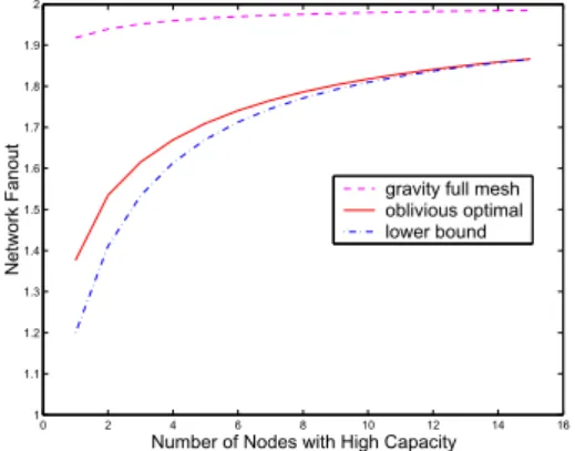
Now let’s consider another example, a network of 16 nodes. The nodes take either one of two access capacities of ratio 10:1. We change the number of nodes
0 2 4 6 8 10 12 14 16 1 1.1 1.2 1.3 1.4 1.5 1.6 1.7 1.8 1.9 2
Number of Nodes with High Capacity
Network Fanout
gravity full mesh oblivious optimal lower bound
with high or low capacities and plot the network fanout in Figure 3. We can see that the oblivious optimal fanout is very close to the lower bound. In fact, as will be shown next, the ratio is bounded by 1.2. So restricting ourselves to oblivious load-balancing does not cause a big loss in capacity efficiency, and we can simplify the load-balancing scheme greatly.
3.4 Oblivious Optimal Network Capacity and the Lower Bound
In the optimal oblivious load-balancing scheme, all the nodes have the same fanout, which is equal to the network fanout, so the total interconnection ca-pacity in the network isLo =Rfo, wherefo is given by Theorem 2. The lower
bound on the total capacity required by any network in order to serve all traffic matrices is given by Theorem 1:Ll= 2(R−r1), where node 1 has the highest
access capacity amongst allN nodes. When r1 ≥PNi=2, we have Lo =Ll, so
we will only consider the caser1 <PNi=2. Letα be the ratio of the minimum capacity in oblivious load-balancing and the lower bound for any network:
α=Lo Ll = R(1 +P 1 i ri R−2ri ) 2(R−r1) = 1 + P 1 i ri R−2ri 2(1−r1 R) . (11)
We study the value ofαin this section.
We have shown that Lo=Rfo<2R and Ll> R, so αis between 1 and 2.
We’d like to find out the maximum value ofα. Equation (11) shows thatαis a smooth function ofri, so the maximum value ofαis achieved when
∂α ∂ri
= 0,∀i. (12)
We can solve for the values ofr∗
i from the above set of equations. But note that
the variablesri, i= 2,3, . . . , N, are completely symmetric in the equations, so in
the solution, they should have the same value. Sinceαis only a function of the
ratios of theri’s, we letr2∗=r3∗=. . .=rN∗ = 1. Now Equation (11) becomes
α= 1 + 1 r1 N−r1−1+ N−1 r1+N−3 2 N−1 r1+N−1 = (N+r1−1)(N−2) N2−2N+ (r1−1)2.
Now we solve forr∗
1: ∂r∂α1 = 0 gives r∗ 1 = 1−N+ p 2N(N−1) (13) and α∗= (N−2) p N(N−1) 2N(√2(N−1)−pN(N−1)). (14) As N increases, α∗ increases and when N → ∞, α∗ → 1
2( √
2 + 1) ≈ 1.207. At the same time, r1 →(√2−1)N = 0.414N. Thus, the ratio of the capacity required by optimal oblivious load-balancing and the capacity lower bound is upper bounded by Equation (14), which is at most 1.2. This shows that in order to serve all valid traffic matrices, oblivious load-balancing requires a total link capacity very close to the minimum total capacity required by any architecture.
4
Related Work
The papers by Applegate et al. [1] and Kodialam et al. [5] both studied using load-balancing to guarantee throughput for a wide range of traffic matrices, from a traffic engineering point of view. Given a capacitated network, they both compared the efficiency of providing service for all traffic matrices vs. for a specific traffic matrix. Applegate et al. [1] used maximum link utiliza-tion ratio as the performance measure and optimizautiliza-tion criteria; Kodialam et al. [5] used the maximum traffic which can be carried by the network. The two measures are equivalent and a ratio of less than 2 was achieved in all their experiments.
Our paper looks at the problem from a network design point of view and tries to find the optimal capacity allocation. We analytically derived that in order to guarantee throughput for all traffic matrices, about twice as much capacity is required compared to the case when the exact traffic matrix is known. This result gives theoretical justification to the upper bound of 2 which has appeared in experiments.
Our work is also complimentary to the above two pieces of work. When designing a network from scratch, or expanding a network’s capacity, our results provide guidelines to the optimal capacity allocation, and can lead the network to grow in an optimal direction. If a network has been built and cannot be changed on a short time scale, the traffic engineering approach can help utilize the network resources more efficiently and alleviate congestion in the network.
5
Conclusion
At first glance, it appears that the VLB architecture is inefficient (because it is based on a full mesh) and introduces long delays (because each packet traverses the network twice). But we believe these fears are probably unfounded. First, we can show that the network is surprisingly efficient – in fact, essentially the most efficient network that can support 100% throughput. We suspect that the actual deployed link capacity of such a network could be much lower than cur-rent networks that can make no such guarantees of service. Second, we believe that the additional delay is unlikely to be a problem to end-user applications. The additional delay is a fixed propagation delay, and so adds nothing to delay variation. In fact, given the efficiency of the network, the queueing delay (and hence delay variation) is likely to be lower than today.
We believe the Valiant Load-Balancing architecture opens up a new dimen-sion in network design. It enables us to design efficient networks that can guar-antee 100% throughput for any traffic matrix, and can continue to do so under a number of element failures. The load-balancing scheme is simple and easy to implement. What’s more, as demonstrated in [10], the amount of excess capac-ity required for fault tolerance is surprisingly small. With VLB, we can build networks to efficiently provide high availability under various traffic conditions and failure scenarios.
Acknowledgment
We would like to thank Kamesh Munagala, Isaac Keslassy and Huan Liu for their insights and very helpful inputs.
References
1. D. Applegate and E. Cohen. Making intra-domain routing robust to changing and uncertain traffic demands: Understanding fundamental tradeoffs. In Proceedings of the ACM SIGCOMM ’03 Conference, 2003.
2. C.-S. Chang, D.-S. Lee, and Y.-S. Jou. Load balanced Birkhoff-von Neumann switches, Part I: One-stage buffering. In Proceedings of IEEE HPSR ’01, May 2001.
3. I. Keslassy, C.-S. Chang, N. McKeown, and D.-S. Lee. Optimal load-balancing. In Proceedings of IEEE Infocom 2005, March 2005.
4. I. Keslassy, S.-T. Chuang, K. Yu, D. Miller, M. Horowitz, O. Solgaard, and N. McK-eown. Scaling Internet routers using optics. Proceedings of ACM SIGCOMM ’03, Computer Communication Review, 33(4):189–200, October 2003.
5. M. Kodialam, T. V. Lakshman, and S. Sengupta. Efficient and robust routing of highly variable traffic. InHotNets III, November 2004.
6. A. Medina, N. Taft, K. Salamatian, S. Bhattacharyya, and C. Diot. Traffic ma-trix estimation: Existing techniques and new directions. In Proceedings of ACM SIGCOMM ’02, Pittsburgh, USA, Aug. 2002.
7. G. Prasanna and A. Vishwanath. Traffic constraints instead of traffic matrices: Ca-pabilities of a new approach to traffic characterization.Providing quality of service in heterogeneous environments: Proceedings of the 18th International Teletraffic Congress, 2003.
8. L. G. Valiant. A scheme for fast parallel communication. SIAM Journal on Com-puting, 11(2):350–361, 1982.
9. Y. Zhang, M. Roughan, C. Lund, and D. Donoho. An information-theoretic ap-proach to traffic matrix estimation. InProceedings of ACM SIGCOMM ’03, pages 301–312. ACM Press, 2003.
10. R. Zhang-Shen and N. McKeown. Designing a predictable Internet backbone net-work. InHotNets III, November 2004.
11. R. Zhang-Shen and N. McKeown. Designing a predictable Internet backbone with Valiant load-balancing (extended version).Stanford HPNG Technical Report TR05-HPNG-040605, April 2005.