Adaptive sequential feature selection in visual perception and pattern recognition

in visual perception and pattern recognition

Von der Fakult¨at f¨ur Mathematik und Informatik der Universit¨at Leipzig

angenommene

D I S S E R T A T I O N

zur Erlangung des akademischen Grades DOCTOR RERUM NATURALIUM

(Dr.rer.nat.)

im Fachgebiet Informatik

vorgelegt

von Master of Philosophy Liliya Avdiyenko geboren am 28.01.1985 in Charkiw, Ukraine

Die Annahme der Dissertation wurde empfohlen von:

1. Professor Dr. J¨urgen Jost (MPI f¨ur Mathematik in den Naturwis-senschaften, Leipzig)

2. Professor Dr. Matthias Bethge (MPI f¨ur biologische Kybernetik, T¨ubingen)

Die Verleihung des akademischen Grades erfolgt mit Bestehen der Verteidigung am 15.09.2014 mit dem Gesamtpr¨adikat cum laude.

Acknowledgments

There are many people who supported me during my PhD and whom I want to thank from the bottom of my heart.

First of all, I am grateful to my supervisor, Prof. Dr. J¨urgen Jost, for giving me an oppor-tunity to develop myself as a scientist in the excellent research environment of his group. I am thankful for everything he taught me, for his guidance, inspiration and openness to new ideas and research directions of his students.

Special thanks go to my “unofficial supervisor”, collaborator and my friend, Dr. Nils Bertschinger. I appreciate our long discussions, his interesting stories about programming languages and inference algorithms and of course his enormous patience and help with formalizing my heuristic reasoning.

Also I want to say my sincere thank you to my colleagues, Wiktor Młynarski, Dr. Tobias Elze, Dr. Hedwig Wilhelm and Dr. Johannes Rauh, for being always there when I needed a piece of advice. In addition, I am grateful to them for proofreading my thesis. There are other colleagues whom I did not mention but whom I am thankful for sharing with me a scientific and nonscientific fun of being a graduate student at our Max Planck Institute. This thesis would not be possible without the financial support of the Max Planck Society that gave me a possibility to do my research as well as present it on various international workshops and conferences.

I would like to mention two magicians of our institute, Antje Vandenberg and Heike Rackwitz, who make lives of foreign PhD students easy and let them feel like at home. I am very grateful for all their support and assistance during my stay at MPI. I want to thank also librarians, a computer group and other institute staff for making it possible to concentrate only on scientific problems.

Last but not least, I would like to thank my friends, my dear Michael, my family and especially my parents, Natalia and Sergii. Their love, belief in me and endless support were with me at every moment of my PhD life and gave me strength to complete this work successfully.

Acknowledgments iii

1 Introduction 1

2 Conventional feature selection 7

2.1 Main approaches to feature selection . . . 7

2.2 Feature selection framework . . . 10

2.2.1 Classification setup . . . 10

2.2.2 General framework of feedforward selection . . . 11

2.3 Selection criteria . . . 12 2.3.1 Misclassification error . . . 12 2.3.2 Gini index. . . 14 2.3.3 Shannon entropy . . . 16 2.3.4 Gain ratio . . . 17 2.3.5 Alpha-entropies. . . 18

2.3.6 Correlation-based feature selection. . . 20

2.3.7 Probabilistic distance measures . . . 22

2.4 Information-theoretical feature selection . . . 24

2.4.1 Definitions . . . 24

2.4.2 Use in solving classification tasks . . . 27

2.5.1 Plug-in approaches . . . 31

2.5.1.1 Density estimation. . . 31

2.5.2 Nonplug-in approaches . . . 41

2.6 Approximated schemes . . . 45

2.7 Conclusion . . . 47

3 Adaptive feature selection 51 3.1 Biological motivation . . . 51

3.2 Adaptive feature selection . . . 54

3.3 Framework . . . 56

3.3.1 Relation to complex adaptive systems . . . 57

3.4 Existing algorithms . . . 58

3.4.1 Local feature selection by decision trees . . . 58

3.4.2 Active testing model . . . 60

3.4.3 Jiang’s sequential feature selector . . . 62

3.5 Adaptive conditional mutual information feature selector . . . 64

3.5.1 Model . . . 64

3.5.1.1 Adaptive vs static selection . . . 66

3.5.2 Estimation . . . 68

3.5.2.1 Density estimation . . . 68

3.5.2.2 Conditional Expectation . . . 72

3.5.2.3 Smoothing . . . 74

4 Experimental investigations of ACMIFS 83 4.1 Data sets . . . 84

4.1.1 Artificial data set . . . 84

4.2 Smoothing. . . 89

4.2.1 Additive smoothing . . . 89

4.2.2 Interpolation with a prior distribution . . . 92

4.3 Comparison with PWFS and ATM . . . 94

4.3.1 General comparison on the artificial data set . . . 96

4.3.2 General comparison on MNIST . . . 97

4.3.3 Behavior in higher dimensions . . . 98

4.4 Combined selection scheme . . . 101

4.5 Conclusions . . . 104

5 Information-theoretical strategies of selective attention 107 5.1 Introduction . . . 107

5.1.1 Existing task-dependent strategies of selective attention . . . 108

5.2 Experimental setup . . . 111

5.3 Tested information-theoretical search strategies . . . 113

5.3.1 Mutual information . . . 113

5.3.2 Conditional mutual information . . . 113

5.3.3 Adaptive conditional mutual information . . . 114

5.4 Sequence statistics . . . 114 5.4.1 Generative model . . . 115 5.4.2 Base likelihood . . . 117 5.5 Experiment . . . 118 5.5.1 Stimuli . . . 118 5.5.2 Presentation software . . . 119 5.5.3 Participants . . . 120 5.6 Results. . . 120 5.6.1 Subject statistics . . . 121

5.6.2 Subject clusters . . . 123 5.7 Conclusions. . . 125

6 Discussion 131

A Appendix 137

A.1 Visual cortex . . . 137 A.2 Artificial dataset. . . 138 A.3 Example of the clicking presentation . . . 139

Introduction

Machine learning is often confronted with high-dimensional data. A common problem is the so-called “curse of dimensionality”, meaning that an amount of data needed to accurately learn parameters of a model grows exponentially with a number of input di-mensions. For this reason, as well as computational issues, feature selection is often used to reduce the data dimensionality to features that are relevant for solving a given problem, such as classification. Moreover, in a situation when a training set is of the limited size, a classifier built on a smaller number of features usually has better generalization ability. Basically, one can distinguish between two types of feature selection algorithms: filters and wrappers [Webb, 1999]. Filters try to reduce the data dimensionality while keeping potential clusters in the data well separated. In this case, the relevance of each feature is evaluated using different measures of a feature’s ability to discriminate between classes. Wrappers also preprocess the data but directly take into account that the resulting features should be useful for a certain classifier. Therefore, features are selected based on the prediction accuracy of the classifier employing these features. This might lead to better results but is usually computationally demanding and prone to overfitting.

For both wrappers and filters, the best feature subset of a certain cardinality can be found using an optimal search strategy. However, a number of possible subsets is exponen-tially large, therefore, testing all of them is computationally infeasible. To tackle this problem, Narendra and Fukunaga proposed the branch and bound method that assumes monotonicity of a selection criterion, which allows to avoid an exhaustive search

[Naren-dra & Fukunaga,1977]. If such an assumption is not valid and the number of features is

large, suboptimal methods have to be used. This class of algorithms includes forward and backward sequential feature selection, where a subset of relevant features is formed by iteratively adding relevant features or removing irrelevant ones, respectively, e. g. [Ding

For feature selection algorithms of the filter type, one of the central questions concerns a selection criterion, i. e. a notion of the feature relevance. An intuitive choice for such criterion is the Bayes error probability of classification using a considered feature [Breiman et al., 1984]. Another popular family of techniques uses different dependency and correlation measures to determine the degree of association between classes and a feature [Mingers, 1987; Duch, 2006]. However, since such measures are usually pair-wise, these techniques are not able to discover high-order dependencies in order to avoid selecting mutually redundant features. As a partial solution, Hall proposed a correlation-based measure punishing features that are highly pairwise correlated with the previously selected features within the sequential feedforward setup [Hall,1999].

Among probabilistic criteria used by filters, selection criteria based on Shannon entropy, a measure of uncertainty in the information theory, are widely used [Duch et al., 2004]. Such criteria select features to reduce uncertainty about the class. Moreover, it was also shown that features that have high mutual information with a class variable, a concept closely related to the Shannon entropy, are indeed useful for classification [Lewis, 1962;

Brown et al., 2012]. Despite numerous estimators of mutual information developed in

the last several decades [Beirlant et al., 1997; Nemenman et al., 2002; Kraskov et al., 2004], its estimation is still considered to be a hard task. However, a problem of feature selection does not require precise values of mutual information. Therefore, even if an estimator is biased, it is sufficient to have the right ordering of features according to their informativeness, which significantly reduces requirements to the quality of estimates. Battiti was one of the first to use mutual information, for sequential feature selection [Battiti, 1994]. However, this involves estimation of the conditional mutual information (CMI), i. e. the amount of information between the feature and the class given the al-ready selected features, which requires multivariate density estimation. To circumvent this problem, Battiti approximated CMI by pairwise mutual information. In addition, his work gave rise to the development of various related approximations of conditional mu-tual information as a criterion for feature selection, e. g. [Yang & Moody, 1999; Kwak

& Choi, 2002b; Fleuret & Guyon, 2004]. Alternatively, kernel density estimation is a

non-parametric technique widely used for multivariate density estimation. It was suc-cessfully applied to estimate CMI and related quantities for the exhaustive search proce-dure [Bonnlander & Weigend,1994] and forward feature selection [Kwak & Choi,2002a;

Bonnlander,1996].

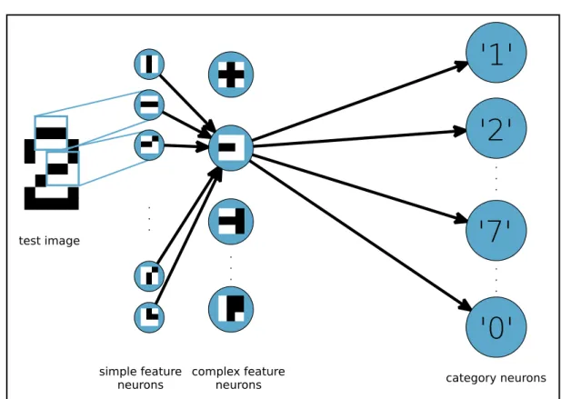
The feature selection algorithm developed in this thesis is inspired by the hypothesis checking mechanism in the human visual system, which is implemented using numerous feedback connections coming from the higher brain areas to the lower ones [Mumford,

1991;Bullier,2001]. Due to the so-called information bottleneck referring to the limited

capabilities of visual processing, only a restricted amount of information can be processed at the same time [Van Essen et al.,1991]. After the first portion of the input is processed

by bottom-up circuits, an initial set of hypotheses about a visual scene is formed in the higher brain areas. If at this stage the scene can not be unambiguously classified, i. e. there is still some uncertainty about the class and therefore no single hypothesis can be chosen, a top-down signal from the higher areas will initiate processing of the next input portion in order to refine the current hypothesis set. Such selection-refinement process will be iteratively repeated until the visual scene is classified.

One can think about small portions of the visual input as its features. Then, the described scheme is nothing else but a feature selection algorithm that selects features relevant for classification of a certain visual scene. Thus, the selection is adapted to an object that should be classified. This phenomenon inspired us to develop a computational algorithm solving a visual classification task that would incorporate such principle, adaptive feature selection. It is especially interesting because usually feature selection methods are not adaptive as they define a unique set of informative features for a task and use them for classifying all objects. However, an adaptive algorithm selects features that are the most informative for the particular input. Thus, the selection process should be driven by statis-tics of the environment concerning the current task and the object to be classified, which in machine learning terms are called a training set and a testing sample, respectively. In this context, the main question we ask in this thesis is whether the proposed adaptive way of selecting features is advantageous and in which situations. Similarly to the visual system where feedback is necessary for recognizing ambiguous objects, we expect that adaptive feature selection should be advantageous for complex classification tasks where it is difficult to define a single static feature subset of a moderate size that would be suf-ficient for the accurate classification. In particular, the usage scenarios for the adaptive selection scheme are the following.

When the structure of data is heterogeneous, one may need different features to discrim-inate between classes, or even different objects belonging to one class may have differ-ent discriminative features. As a result, it is very likely that no single small subset of features is good enough for classification of all observations. One can partially over-come this problem by having a collection of all relevant feature subsets. This, however, will lead to an increase in the classifier complexity, which in turn will lead to its poor performance, unless a large amount of training data is available for training a classifier in high-dimensional space [Raudys & Jain, 1991]. Thus, conventional feature selection schemes, which select a fixed subset of features before they are handed to a classifier, can be inefficient.

In addition to the case with heterogeneous data, we expect the adaptive approach to feature selection to be advantageous when the amount of available training data is limited and the number of features exceeds the number of training samples. If features are selected in the adaptive way, their relevance is judged only for a small subregion of the input space where a testing sample lies. At the same time, static schemes look for features that are globally

relevant, i. e. features with the high discriminative power for all samples from a training set. Therefore, it is very probable that in the undersampled regime, when the training set does not fully represent the true data distribution, estimates of the local relevance would be more accurate than those of the global relevance. As a result, quality of the adaptively selected features would be better and in order to reach the same classification accuracy, one would need a smaller number of adaptively selected features comparing to static selection schemes.

Thus, in cases when it is difficult to find a small fixed subset of relevant features, we propose to use different features for every testing sample, i. e. select the informative features in an “adaptive” manner. By adaptivity we mean that for a certain testing sample every selected feature should be maximally relevant for its classification given values of the already selected features observed on this testing sample.

The idea of adaptivity was used by Geman and Jedynak in their active testing model

[Ge-man & Jedynak, 1996] where they sequentially select tests in order to reduce uncertainty

about the true hypothesis. For their problem domain, they assumed that features are con-ditionally independent given the class, which simplified the estimation. Jiang also used an adaptive scheme [Jiang, 2008], however, without conditioning on the already selected features, which are employed only to update a set of currently active classes. In contrast to these schemes, we adaptively select features taking into account high-order dependencies between them.

Therefore, we propose an adaptive feature selection algorithm that utilizes a selection criterion based on Shannon entropy. Applied to a classification task, our adaptive feature selection algorithm sequentially adds features one by one to a subset of features in order to reduce uncertainty about a class of a certain testing sample. In information-theoretical terms, a selection criterion is the mutual information of a class variable and a feature-candidate conditioned on the already selected features, which take values observed on the current testing sample. Hence, we call it adaptive conditional mutual information feature selector (ACMIFS). For its estimation, we utilize a plug-in estimator based on kernel density estimates with the proposed here adaptive smoothing. Even though the mutual information is hard to estimate in general and from small data sets especially, practical investigations of the algorithm show that it is able to select informative features in high dimensions.

It is well-established that there are two factors affecting shifts of the visual attention: vi-sual stimuli themselves and a task. While the influence of image statistics on the viewing behavior is intuitive, a fact that a saccade sequence differs depending on a task had to be proven experimentally [Yarbus, 1967;Rothkopf et al., 2007;Betz et al.,2010]. How-ever, the question remains what kind of strategy people use to decide what is relevant for a task, e. g. simple heuristics or complex algorithms based on the ideas of infor-mation theory etc. Surprisingly, despite their computational complexity, statistical and

information-theoretical definitions of the task-relevance are often used in the state-of-the-art algorithms predicting eye movements [Najemnik & Geisler, 2005; Itti & Baldi,

2006; Renninger et al., 2007]. Inspired by a process that selects relevant sources of the

visual information, our adaptive feature selection scheme can also be seen as a visual search strategy underlying eye movements while performing a task. Therefore, further we investigate the next question, namely whether the proposed information-theoretical selection scheme, which is a computationally complex algorithm, is utilized by humans while they perform a visual classification task. For this, we constructed a psychophysical experiment where people had to select image parts that in their opinion are relevant for classification of these images. We present the analysis of behavioral data where we in-vestigate whether human strategies of task-dependent selective attention can be explained by a simple scheme based on the pairwise mutual information, a more complex feature selection algorithm based on the conventional static conditional mutual information and the proposed here adaptive feature selector that mimics a mechanism of the iterative hy-pothesis refinement.

The main contribution of this work is the adaptive feature selection criterion based on the conditional mutual information, as well as its non-parametric estimation that does not presume any problem-specific assumptions. Moreover, it is shown that such adaptive selection strategy, being inspired by the attentional modulation of task-relevant parts of a visual scene, is indeed used by people while performing visual classification.

The thesis is organized in the following way. Chapter2reviews the conventional feature selection. Main approaches to dimensionality reduction in general and feature selection in particular are discussed in Section2.1. Further, in Section2.2, we introduce a general framework of sequential feature search which is used in Section 2.3 to present differ-ent selection criteria. Information-theoretical feature selection together with appropriate estimation techniques are reviewed in Section2.3and in Section2.4, respectively.

Chapter3 starts with the biological motivation and the general idea of the adaptive ap-proach to feature selection, given in Section3.1 and Section 3.2, respectively. Section 3.3 introduces a framework of adaptive feature selection, which is followed by Section 3.4 presenting a review on existing algorithms utilizing this approach to dimensionality reduction. After that, in Section3.5, the proposed adaptive conditional mutual informa-tion feature selector is presented. In particular, Subsecinforma-tion3.5.1introduces the model, its estimation using kernel density method with the adaptive smoothing is described in Sub-section3.5.2. Results of practical investigations are provided in Chapter4, where ability of ACMIFS to select relevant features in general and especially in high dimensions is examined. In addition, Section4.3 presents comparison of ACMIFS with two static and adaptive feature selectors based on conditional mutual information, Parzen window fea-ture selector [Kwak & Choi,2002a] and active testing model [Geman & Jedynak,1996]. Further, an alternative selection scheme combining ACMIFS and active testing model in

order to reduce computational complexity is proposed in Section4.4. The discussion of advantages of adaptive feature selection is given in Section4.5.

Chapter5presents the psychophysical experiment where human strategies of task-dependent selective attention are investigated. Section5.1 reviews existing strategies of attentional selection with the emphasis on the task-dependent ones. Further, in Section5.2, we de-scribe an idea of the clicking experiment. Section 5.3 provides details of three tested information-theoretical strategies based on mutual information, static and adaptive condi-tional mutual information of a class with an image patch. Section5.4presents a statistical method that is used to compare these strategies with respect to their explanatory power of the observed behavioral data. Technical details of the experimental setup are described in Section5.5. Section5.6presents the analysis and interpretation of the clicking experi-ments. Finally, the general discussion is provided in Chapter6.

Conventional feature selection

2.1

Main approaches to feature selection

Feature selection algorithms reduce dimensionality of the input space by picking a small number of relevant features from the initial feature set. As representatives of dimension-ality reduction techniques, they are used to solve a so-called “curse of dimensiondimension-ality” problem, meaning that there exists exponential dependence between the dimension of the input and the amount of data required to learn model parameters. Thus, decreasing the input dimensionality should ease a learning process. Moreover, a model with fewer parameters usually has better generalization ability.

Besides feature selection, there is another method of reducing dimensionality called fea-ture extraction. This family of techniques performs transformation of the initial input space to the space of reduced dimensionality, which usually has also some desired prop-erties like orthogonality or independence of new features etc. It is worth to mention that some feature extraction algorithms expand the initial input dimensionality in a way that a learning problem becomes simpler in the transformed space [Broomhead & Lowe, 1988;

Simoncelli et al.,1992;Lewicki et al.,1998]. Since we are interested in selecting features

and not in their transformations, we will speak further exclusively about feature selection algorithms. The review of feature extractors can be found for example in [Liu & Motoda,

1998; Guyon et al., 2006]. The most prominent representatives in pattern recognition

are principal component analysis [Pearson, 1901; Jolliffe, 1986], independent compo-nent analysis [Hyv¨arinen et al., 2004] and sparse coding due to its biological plausibility and connection to receptive field properties of neurons in primary visual cortex [Foldiak,

Feature selection algorithms can be divided into two main classes: filters and wrappers [Webb, 1999]. The filters look for a minimal subset of features that can maximally en-hance classification, i. e. discriminate between samples belonging to different classes with the minimal error. In order to evaluate a discrimination power of a feature subset, different metrics are used such as various distance measures between classes, dependency measures between features and classes etc. Note that these metrics are not restricted to a particular classification method, therefore, selected features can be used for training any classifier. However, it can also be considered as a drawback, since the resulting feature subset may be suboptimal for the chosen classifier. An extensive overview of distance measures used by the filters will be presented later in Section2.3.

Comparing to the filter methods, the wrappers select features that are useful for a cer-tain classifier [Kohavi & John,1997]. A goodness of a feature subset is measured by the prediction accuracy of a classifier employing these features. Thus, one can be sure that the selected features will indeed improve the quality of classification. However, there is a danger of overfitting. This means that the features are selected in the way to provide the best classification performance on the training data which might however lead to poor accuracy on the previously unseen test data. Moreover, these methods are rather compu-tationally expensive, since in order to find the best feature subset a classifier should be run as many times as there are different subsets under consideration. Among represen-tatives of wrappers, there are a recursive algorithm for support vector machines [Guyon

et al., 2002], a wrapper feature selector for Bayesian networks [Singh & Provan, 1995],

Kohavi’s sequential feature selection for a general classifier [Kohavi & John, 1997] etc. Linear discriminant analysis can also be seen as a wrapper which performs feature selec-tion while building a linear classifier on input features [Fisher,1936]. Since the classifier itself is simple and the only made assumption is that data drawn from each class are normally distributed, this technique is often used as a filter [McLachlan,2004].

There is another type of feature selectors called embedded methods [Duch,2006]. They can be considered as a subtype of the wrappers because during the selection process they take also into account a classifier to be used. However, instead of directly employing re-sults of classification, they rather use knowledge about the structure of a classifier while evaluating how good different feature subsets are. Thus, compared to the wrappers, the embedded methods are less computationally complex and less prone to overfitting. Exam-ples of such methods are a feature selector for support vector machines, which minimizes a generalization bound [Weston et al.,2000], decision trees and artificial neural networks. In each case, one can look for the best feature subset of a certain cardinality using an op-timal search strategy which assumes evaluating all possible feature subsets and choosing the best one [Reunanen,2006]. Since the number of such subsets is exponentially large, testing all of them is infeasible unless a number of the initial features is small. A good example of the optimal strategy avoiding an exhaustive search is the branch and bound

method [Narendra & Fukunaga, 1977; Yu & Yuan, 1993; Somol et al., 2004]. The key point here is monotonicity of a selection criterion. It means that if for two sets

A

and

B

,

A

⊂

B

, then the goodness of the set

A

is not larger than the goodness of the set

B

. Using such assumption together with backward selection, i. e. iterative elimination of fea-tures from the initial set, one can disregard some subsets on the intermediate iterations if their discriminability is low. For references to selection criteria which are monotonic and therefore can be used in combination with the branch and bound search, see the review on feature selection and extraction of Webb [Webb,1999].

We would rather consider a general case and assume that a selection criterion does not sat-isfy the monotonicity assumption. Then, suboptimal methods have to be used. This class of algorithms includes feedforward and backward sequential feature selection which use the greedy search strategy [Webb, 1999;Jain & Zongker, 1997]. The feedforward algo-rithms start with an empty feature set and iteratively add features, which are relevant with respect to the features selected on the previous iterations [Whitney,1971]. As was already mentioned above, the backward approach starts with the full feature set and on every it-eration removes features that are the least useful in the current subset of the remained features [Marill & Green,1963;Abe,2005]. A popular backward method is the Markov blankets algorithm that sequentially removes irrelevant features. A featureF_k is said to be irrelevant if it has a Markov blanket, i. e. there exists such a feature subset

F

0 that if

F_kis conditioned on this subset, then it is independent of all remaining features [Koller &

Sahami,1996;Tsamardinos et al.,2003].

The suboptimality of sequential methods comes from the fact that they do not explicitly look for the best feature subset. They rather try to find a feature or several features that can improve discriminability of the current subset as much as possible. The resulting feature subsets found by optimal and suboptimal approaches will differ a lot if there are high-order dependencies between features. Comparing feedforward and backward algorithms, the latter can theoretically show better results. Assuming that there are some complemen-tary features which are informative only together and not alone, the feedforward methods would not choose any of these features at all, and therefore, they would not have a chance to evaluate the goodness of these features together. In the case of the backward methods, it is more likely that such features will be included in the final feature subset, because eliminating any of them from the feature set will result in decrease of its discrimination power. However, in practice, the backward methods are used less often. Feature subsets on early iterations are of large cardinality, which makes the evaluation of their relevance complicated. Moreover, practical studies have not shown that the backward approach pro-duces always better feature subsets when compared to the feedforward approach [Aha &

Bankert, 1996;Kudo & Sklansky,2000]. Sequential floating feature selectors belong to

the class of algorithms that assume alternation of feedforward and backward steps while searching for the informative feature subsets. Though, they have proven quite efficient, the applicability of floating search methods is limited due to their exponential complexity

[Pudil et al., 1994;Jain & Zongker, 1997]. For a review on various search methods for feature selection see [Reunanen,2006;Somol et al.,2007].

A feature selection algorithm, which is proposed later in this thesis, is inspired by the hypothesis checking mechanism in the visual system. It iteratively selects small parts of a visual input for the detailed processing in order to refine hypotheses about objects present in the visual scene. Keeping a parallel to this mechanism of the visual system, we adopt a sequential feedforward approach to feature selection. Further, as a task we consider image classification, therefore, all feature selection techniques will be presented in connection to classification. Hence, a model describing data will refer to an abstract classifier. For completeness, we name some examples of features selection methods for regression. These are regression trees [Breiman et al., 1984], regularization schemes [Tibshirani, 1996; Zou & Hastie, 2005] and various filters using correlation or entropy between features and a dependent variable as a measure of the feature relevance, e. g. [Hocking,1976;Carmona et al.,2011].

2.2

Feature selection framework

2.2.1

Classification setup

Let us introduce a standard classification setup and a conventional scheme of feature selection within this setup.

Suppose we have a space of possible inputs

F

= ×n

i=1

F

i, i. e. each input is an n -dimensional feature vector f= (f1, . . . ,fn), where the ith feature takes values fi∈

F

i. Our notion of feature is rather general. For example, for the image classification task, features can be quite simple, such as gray-values of certain pixels, or more sophisticated, such as frequencies of some objects on an image. Feature combinations are considered as a random variableF with a joint distribution on

F

1× · · · ×

F

nand the observationfis drawn from that distribution.

Furthermore, each observation has an associated class labelc∈

C

={c₁, . . . ,c_m}. The task of the classifier is to assign a class label to each observationf. Thus, formally it is considered as a mapφ:

F

→

C

or, more generally, as assigning to eachfthe conditional

probabilitiesp(c|f)of the classesc. To learn such classification, we are given a training set

X

={(xi,ci)}Ti=1of labeled observations, which are assumed to be drawn independently

from the distribution relating feature vectors and class labels. Then, the goal is to find a classification ruleφthat correctly predicts the class of future samples with unknown class

it asc=φ(ξ). Feature selection then means that for this particular task only a subset of

features rather than the full feature vector is used.

2.2.2

General framework of feedforward selection

According to the conventional sequential feedforward feature selection for classification, a featureF_αi+1 selected on the(i+1)th step should maximize some selection criterionS, i. e.:

αi+1=arg max

k

S(C,F_α1, . . . ,F_αi,F_k), F_k∈ {F₁, . . . ,F_n} \ {F_α1, ...,F_αi}, _(2.1)

where Fα1, . . . ,Fαi is a subset of the features selected before the (i+1)

th _iteration. In-tuitively, the selection criterion S should favor such features that arerelevant for clas-sificationwith respect to the variableC. At the same time, it is desirable that the final feature subset is of the minimal size, therefore, the selected features should be maximally

non-redundant with respect to each other.

Let us formalize the concepts of relevance and redundancy. Suppose we are given an unlabeled sample. Before any feature is observed, we are completely uncertain about a class label of this sample. LetU(C) be some measure of uncertainty about the variable

C. Then, a feature F_k is said to be relevant for classification if given this feature the uncertainty about the class of some hypothetical sample will be reduced, i. e. U(C)<

U(C|F_k). Note that feature selection is performed before classification and therefore the selected features should be discriminative for any sample that we would have to classify in the future.

Suppose that we have already selectedifeatures and letFi denote a subset of these fea-tures, Fi ={F_α1, ...,F_αi}. At this stage, the current uncertainty about the class can be expressed asU(C|Fi). Then, the feature F_k is both relevant for classification and non-redundant w. r. t. the already selected features if knowing this feature the current un-certainty about the class will be reduced:U(C|Fi)<U(C|F_k,Fi). Thus, the criterion for selecting a feature on the iteration(i+1)can be formulated in the following way:

αi+1=arg max

k

S(C,Fi,F_k) =arg max k {

U(C|Fi)−U(C|F_k,Fi)}. (2.2)

In addition to a search strategy, a key issue in feature selection is the choice of a selection criterion, which in the framework of uncertainty reduction corresponds to the choice of the uncertainty functionU(·). Breiman and coauthors, while working on decision trees, which can also be considered as feature selectors, developed a set of desired properties for uncertainty functions and proposed several examples satisfying these properties [Breiman et al.,1984].

Denoting a probability of the class c_j after the ith iteration as p(c_j|fi), the uncertainty

U(C|Fi)is defined as a nonnegative function which depends on p(c1|fi), . . . ,p(cm|fi). In our notation,fi stands for a vector of particular realizations of the selected featuresfi=

{F_α1 = f_α1, ...,F_αi= f_αi}. Then,U(C|Fi)should have the following properties [Breiman et al.,1984]:

1. U(C|Fi) =max, if all classes are equiprobable, i. e. p(cj|fi) =p(cj0|fi),∀j,j0= 1, . . . ,m.

2. U(C|Fi) =min, if all samples belong to one class, i. e. p(c_j|fi) =1 and p(c_j0|fi) = 0,∀j06= j.

3. U(C|Fi)is symmetric inp(c1|fi), . . . ,p(cm|fi).

2.3

Selection criteria

Here, we present various uncertainty functions which satisfy the above stated properties and are widely used for feature selection. The review is given with respect to the presented setup of the sequential feedforward feature selection for pattern classification.

2.3.1

Misclassification error

While solving a classification problem, the goal is to build a classifier with the best accu-racy. So intuitively an uncertainty function should depend on the misclassification error. Following Breiman and coauthors, let us define the misclassification error fori selected features with the 0-1 loss function [Breiman et al.,1984]:

U(C|Fi) =

∑

Fi p(fi) 1−max j p(cj|f i₎ , (2.3) where∑ Fi stands for ∑ Fα1 · · ·∑ Fαi

for brevity. Note that the expression (2.3) is in fact the Bayes error probability, which is the lowest possible error probability for a given classification problem:

∑

Fi p(fi) 1−max j p(cj|f i₎ =

∑

Fi p(fi) m

∑

j=1,j6=j0 p(cj|fi) ! =

∑

Fi m

∑

j=1,j6=j0 p(c_j)p(fi|c_j), (2.4)

wherec_j0 is the winning class, i. e. p(c_j0|fi) =max j p(cj|f

i_).

Using the misclassification error as an uncertainty function, the corresponding feature selection criterion has the following form:

αi+1=arg max k { U(C|Fi)−U(C|F_k,Fi)}= arg max k {−

∑

Fi p(fi)max j p(cj|f i_{) +}

∑

Fi

∑

_Fk p(f_k,fi)max j p(cj|fk,f i_)}. (2.5)

This selection criterion is obviously useful for selecting features that can discriminate well different classes. Since in practice neither an ideal classification rule nor posterior distributions p(c_j|f_k,fi)are known, different approximations should be used. For exam-ple, one can employ nonparametric techniques of density estimation such as the kernel density method for estimating class-conditional pdfsp(f_k,fi|c_j)and then apply the Bayes rule to obtain the posteriors [Fukunaga & Hummels,1987;Yang & Hu, 2012]. k-nearest neighbor method is also used to estimate a selection criterion based on the Bayes er-ror probability by margin-based feature selection algorithms such as Relief, which try to weight available features in a way so that a margin between classes is maximal [Kira

& Rendell, 1992; Gilad-Bachrach et al., 2004; Sun, 2007; Yang & Hu, 2012]. Another

approach to the estimation problem is introducing simplifying assumptions about the in-volved pdfs such as being Gaussian etc [Bruzzone & Serpico,1998].

Despite its simplicity and intuitive usefulness for solving classification problems, the se-lection criterion based on the misclassification error has a major disadvantage as an uncer-tainty function. It does not explicitly favor situations where the posterior of some classes approaches 0 or 1, which happens due to the linear dependence between the uncertainty and(max

j p(cj|fk,f i_)).

Let us consider a two-class problem. In this case, the uncertainty function based on the misclassification error (2.3) is the following:

U(C|Fi) =

∑

Fi

p(fi)(1−max{p(c1|fi),p(c2|fi)}) =

∑

Fi

p(fi)min{p(c1|fi),p(c2|fi)}. (2.6)

Keeping in mind thatU(C|Fi) = ∑ Fi

p(fi)U(C|fi), Figure2.1depictsU(C|fi)as a function of p(c1|fi), illustrating its linear behavior. Therefore, as the class posterior distribution

becomes less uniform, i. e. whenp(c₁|fi)decreases on the interval[0,0.5)or correspond-ingly increases on the interval(0.5,1], the functionU(C|Fi)decreases just linearly.

0 0.25 0.5 0.75 1 0 0.5 1 misclass. error Gini index Shannon entropy

Figure 2.1: Uncertainty functionU(C|fi)based on misclassification error, Gini index and Shannon entropy plotted againstp(c₁|fi)for a two-class problem.

2.3.2

Gini index

Following further the approach of Breiman and coauthors, we introduce a family of un-certainty functions so that resulting selection criteria give more weight to less uniform class posterior distributions, i. e. whenp(c_j|·) =1 or p(c_j|·) =0.

For this, the desired property forU(C|Fi)would be to decrease faster than linearly. This can be ensured ifU(C|Fi) is strictly concave. So forU(C|Fi), which is continuous on the interval [0,1], and p(c1|fi)∈[0,1], the second derivative of the function should be

negative,U00(C|Fi)<0.

Let us proceed with construction of the improved uncertainty function. Recalling three general requirements, we rewrite them for the two class problem. Since p(c₂|fi) =1−

p(c₁|fi), we can consider thatU(C|Fi)depends only onp(c₁|fi):

1. U(C|Fi) =max, if p(c₁|fi) =0.5.

2. U(C|Fi) =min, ifp(c₁|fi) =1 or p(c₁|fi) =0. Without loss of generality (w.l.o.g.) we can require that the minimum value ofU(p(c1|fi))is 0.

3. U(C|Fi)is symmetric, i. e.U(c1|fi) =U(c2|fi).

And we add the new requirement 4. U00(C|Fi)<0.

The simplest example of the concave function is a quadratic polynomial, which gives

U(C|fi) =ap(c1|fi)2+bp(c1|fi) +c.

The second and the forth requirements give c =0, a+b=0 and a< 0, respectively. Assuming w.l.o.g. thata=−2, the uncertainty function is of the form:

U(C|Fi) =

∑

Fi p(fi) 2(−p(c1|fi)2+p(c1|fi)) =

∑

Fi 2p(fi) −p(c1|fi)(1−p(c2|fi)) +p(c1|fi) =

∑

Fi p(fi) 2p(c1|fi)p(c2|fi) , (2.7)

which is known as the Gini index, a measure of statistical dispersion proposed by Corrado Gini [Gini, 1912]. The general form of the Gini index for a multiclass problem has the following form: U(C|Fi) =

∑

Fi p(fi) m

∑

j=1 m

∑

j0=1,j6=j0 p(cj|fi)p(cj0|fi) =

∑

Fi p(fi) 1− m

∑

j=1 p(cj|fi)2 ! . (2.8)

Due to simplicity of its estimation and correspondence to the desired properties of the uncertainty function (see Figure2.1), this criterion is widely used in decision tree con-struction [Breiman et al.,1984] and [Gelfand et al.,1991].

There is a modified version of the Gini index which is widely used for feature selection in the field of text classification [Shang et al.,2007;Yang et al.,2011]. Let us rewrite the feature selection criterion in the following way:

k=arg max k U(C|Fi)−U(C|F_k,Fi) =arg min k U(C|F_k,Fi) = arg min k ( p(f_k,fi) 1− m

∑

j=1 p(cj|fk,fi)2 !) . (2.9)

First, the criterion2.9is simplified to arg maxk

( p(f_k,fi) ∑m j=1 p(cj|fk,fi)2 ) , wherep(f_k,fi)

is further replaced withp(f_k,fi|c_j)2:

k=arg max k ( m

∑

j=1 p(f_k,fi|cj)2p(cj|fk,fi)2 ) . (2.10)

The replacement is done in order to favor more class-specific features, i. e. features with low marginal probabilities but high class-conditional probabilities for some c_j. This is especially useful when classes are unbalanced.

2.3.3

Shannon entropy

In terms of information theory, a measure of uncertainty about the outcome of a random variable is Shannon entropy [Shannon & Weaver, 1949]. For a random variable X, it is defined by the following expression:

H(X) =−

∑

X

p(x)logp(x). (2.11)

The uncertainty about the class label after selecting certain featuresFα1, . . . ,Fαi is mea-sured by the conditional entropy:

U(C|Fi) =H(C|Fi) =−

∑

Fi m

∑

j=1 p(c_j,fi)logp(c_j|fi). _(2.12)

Shannon entropy has all four desired properties of the uncertainty function: it takes its maximum when the class-conditional distribution is uniform, it equals zero when the pos-terior of one of the classes is 1, and it is strictly concave:U00(C|Fi) =−∑

Fi

p(fi) ∑m

j=1 1

p(cj|fi₎< 0. This can be seen on Figure2.1plotting Shannon entropyH(C|fi)against p(c1|fi)for a

two-class problem.

Rewriting the selection criterion with Shannon entropy as the uncertainty function, we obtain:

S(C,Fi,F_k) =U(C|Fi)−U(C|F_k,Fi) =H(C|Fi)−H(C|F_k,Fi) =I(C;F_k|Fi), (2.13)

whereI(C;F_k|Fi) is the mutual information between the class variableC and the feature

F_kafter selectingifeaturesFi. It tells how much one can learn aboutCafter observing an outcome of the featureF_k, which is usually measured in bits, or equivalently how certain one can classify the samples after selectingF_kgiven already selected featuresF₁, . . . ,F_i. Using the definition of mutual information, the selection criterion can be further rewritten in the following way:

S(C,Fi,F_k) =I(C;F_k|Fi) =

∑

Fi

∑

_Fk m

∑

j=1 p(c_j,f_k,fi)log p(cj,fk|f i₎ p(c_j|fi_)p(f k|fi) , (2.14)

which can be interpreted as the expected value of the logarithmic function of p(cj,fk|f i₎ p(cj|fi_)p(fk|fi₎, a degree of correlation between the variablesCandF_konce the featuresFiare selected. Mutual information as a selection criterion is very often used in feature selection algo-rithms as it provides a natural measure of interdependence between features and the class,

e. g. [Lewis,1962;Quinlan,1986;Battiti,1994;Kwak & Choi,2002a;Fleuret & Guyon,

2004; Peng et al., 2005], and it is invariant under invertible transformations of involved

variables [Rez¯a,1961;Kraskov et al.,2004]. The major difficulties in using mutual infor-mation concern its estiinfor-mation. As the feature selection criterion proposed in this thesis is based on Shannon entropy or analogously on the mutual information, a detailed discus-sion of entropy-related issues will be presented later.

2.3.4

Gain ratio

The selection criterion based on mutual information has a practical problem when fea-tures are discrete. There is a bias in selection towards feafea-tures with many values. The reason is the following. Since the mutual information is a symmetric measure, then

I(C;F_k|Fi) =H(F_k|Fi)−H(F_k|C,Fi). As a result, a feature with many values has a high entropyH(F_k|Fi)that could lead to a high value of the mutual information.

An intuitive solution to this problem is to punish features with high entropy values. Thus, the proposed modified uncertainty function, which is in the decision tree community called “Gain ratio” [Quinlan,1993], is a normalized form of (2.13), the selection criterion using Shannon entropy as the uncertainty function:

S(C,Fi,Fk) = U(C|Fi)−U(C|Fi,F_k) H(F_k|Fi₎ = H(C|Fi)−H(C|Fi,F_k) H(F_k|Fi₎ = I(C;F_k|Fi) H(F_k|Fi₎ . (2.15) This expression measures the ratio between the informativeness of the featureF_kfor clas-sification and its entropy. However, the measure becomes unstable once the entropy of some features starts approaching zero, i. e. when the feature has only one or very few val-ues. Experiments using the gain ratio show that features with high entropy are punished too much and almost never chosen [Mingers, 1987]. At the same time, a similar idea has been successfully used for normalizing the mutual information between two features

I(F_i,F_j)as a component of the selection criterion (2.13) [Estevez et al.,2009]:

k=arg max k ( I(C;F_k)−1 i i

∑

q=1 I(F_k;F_q) min{H(F_k),H(F_q)} ) . (2.16)

Another example is the symmetrical relevance criterion which uses the joint entropy

H(C,F_αq,F_k)as a normalization factor for the multivariate mutual informationI(C;F_αqF_k)

[Meyer & Bontempi,2006]:

k=arg max k ( i

∑

q=1 I(C;F_αqF_k) H(C,F_αq,F_k) ) . (2.17)

Both above-mentioned criteria are approximations of2.13. A detailed overview of various approximations of entropy-based selection criteria will be presented further in Section2.6. For a review on information-theoretical selection criteria using different normalization techniques see [Duch,2006].

2.3.5

Alpha-entropies

Shannon entropy assumes a certain trade-off between contributions from the main mass and tails of a distribution and events that occur too often or too rare do not influence much the entropy. So-calledα-entropies, R´enyi entropy [R´enyi,1961] and Tsallis entropy

[Tsal-lis,1988], are generalized versions of Shannon entropy that give a possibility to control

this trade-off explicitly. The α-entropy of some variable X is a function of ∑_X p(x)α,

where the parameterαcorresponds to the degree of inhomogeneity in the structure of the

probability distribution ofX [Holste et al., 1998]. That is, α controls a contribution of

events of different frequencies to the sum, i. e. for largeαonly the high-frequency events

contribute, whereas for smallαall events are weighted more uniformly. Due to this

flexi-bility,α-entropies are widely used to describe behavior of complex systems in such fields

like statistical thermodynamics, e. g. [Ramshaw,1995], nonlinear dynamical systems, e. g. [Grassberger & Procaccia,1983], evolutionary programming, e. g. [Stariolo & Tsallis, 1996] etc.

α-entropies are also used as uncertainty functions in feature selection. For theα-entropy

H_α(C|Fi), the parameter α allows to control a trade-off between the purity of the class

posterior distribution, which is considered to be the best criterion to optimize from the Bayesian viewpoint [Duch,2006], and reducing the average uncertainty. The less uniform posteriors, i. e. when the posterior of one of the classes is around 1, can be achieved with

α→0. In this case, all events contribute to the entropy and it will be significantly reduced

only whenp(c_j|fi)→1. Both R´enyi and Tsallis entropies are identical to Shannon entropy forα→1. Let us take a closer look at these parameterized entropies.

The uncertainty functionU(C|Fi)using the R´enyi entropy is

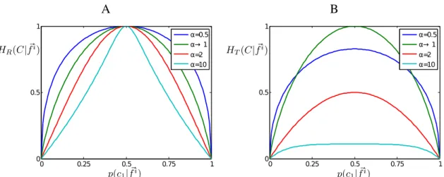
H_R(C|Fi) =

∑

Fi p(fi) 1−αlog m

∑

j=1 p(c_j|fi)α ! , α>0,α6=1, (2.18)

leading to the following feature selection criterion (note its resemblance to mutual infor-mation): S(C,Fi,F_k) =H_R(C|Fi)−H_R(C|Fi,F_k) =

∑

Fi

∑

_Fk p(fi,f_k) 1−α log     m ∑ j=1 p(c_j|fi)α m ∑ j=1 p(c_j|fi_,f k)α     (2.19)

R´enyi entropy has the first three desired properties of the uncertainty function but, in contrast to the concave Shannon entropy, it is concave only for α ∈(0,1) and neither

concave nor convex forα>1. Figure2.2illustrates the behavior of the quantityHR(C|fi) as a function ofp(c₁|fi)for different values ofαfor a two-class problem. One can see that

for smallαthe decrease in entropy will be significant only if p(c1|fi)→1 orp(c1|fi)→0.

However, for large α a slight move away from the uniform posterior, i. e. away from

p(c₁|fi) =0.5, causes noticeable entropy reduction.

A B 0 0.25 0.5 0.75 1 0 0.5 1 α=0.5 α→ 1 α=2 α=10 0 0.25 0.5 0.75 1 0 0.5 1 α=0.5 α→ 1 α=2 α=10

Figure 2.2: A: R´enyi entropy as the uncertainty function plotted against p(c1|fi) for different

values ofαfor a two-class problem. B: Tsallis entropy as the uncertainty function plotted against p(c1|fi)for different values ofαfor a two-class problem.

Tsallis entropy is a generalization of Boltzmann-Gibbs entropy from statistical mechanics and for the distributionp(c|fi)it is defined as follows:

H_T(C|Fi) =−

∑

Fi p(fi) 1−α 1− m

∑

j=1 p(c_j|fi)α ! , α>0,α6=1. (2.20)

As Tsallis entropy is always concave, it satisfies all four desired features of the uncertainty function. However, compared to Shannon entropy, it is nonadditive. Additivity is one of the algebraic properties of the uncertainty measure requiring the joint entropy of two independent events to be a sum of their marginal entropies, i. e.H(X,Y) =H(X) +H(Y)

[Acz´el & Dar´oczy,1975]. For Tsallis entropy, we have:

H_T(X,Y) =H_T(X) +H_T(Y) + (1−α)HT(X)HT(Y), (2.21)

where (1−α) indicates a degree of deviation from an additive system. Nonadditivity

can be useful if the system is known to have nonlinear long-range couplings between its elements [Caruso & Tsallis,2008].

Figure2.2 plots Tsallis entropy H_T(C|fi)against p(c₁|fi) for different values ofα for a

two-class problem. For small α, as in case of R´enyi entropy, HT vanishes only when

p(c_j|fi)→1. For large values of α, the Tsallis entropy of the system does not change

much by moving away from the uniform posterior. Such immunity to small changes in the class conditional probability distribution can help to achieve better generalization and robustness against noise.

Using Tsallis entropy as the uncertainty function, the feature selection criterion has the following form S(C,Fi,F_k) =HT(C|Fi)−HT(C|Fi,Fk) =

∑

Fi

∑

_Fk p(fi,f_k) 1−α m

∑

j=1 p(cj|fi)α−p(cj|fi,fk)α . (2.22)

As uncertainty functions in decision tree construction, R´enyi and Tsallis entropies were used for example by [Maszczyk & Duch, 2008;Lima et al., 2010]. It was reported that due to the possibility to adjust to a structure of the probability distribution describing a given problem, constructed trees are usually smaller and have better performance than trees using the Shannon entropy. Moreover, this class of entropies is attractive for general feature selection due to the reduced computational complexity compared to the Shannon entropy [Liu & Hu,2009;Lopes et al.,2009].

2.3.6

Correlation-based feature selection

The list of the selection criteria presented above is not exhaustive. Among others, there are criteria that do not formally fit in the framework of uncertainty reduction. The first class of such approaches are based on dependency measures between variables.

As an alternative to the selection criterion based on mutual information (2.13), it was suggested to use theχ2-statistic instead [Hart,1985]. Similarly to mutual information,χ2

-statistic measures a degree of dependence between a class and discrete features. However, this measure is usually used only for ranking, which assumes evaluating relevance of each feature alone and not together with other features. As a result, features that are relevant only in combination with other features will not be selected and a resulting feature subset will be likely redundant.

Theχ2-statistic for a featureFkafter selectingifeatures is defined in the following way:

S(C,F_k,Fi) =χ2(C,Fk) = r

∑

l=1 m

∑

j=1 (T_{l j}−E_{l j})2 E_{l j} , Fk∈

F

\ {F1, . . . ,Fi}, (2.23)

wherer is a number of the discrete values of the feature F_k; T_{l j} is a number of training samples belonging to the classc_jand featureF_ktaking the value f_l. E_{l j}= TlTj

T whereTlis a number of samples withF_k equals f_l, Tjis a number of samples belonging to the class

c_jand finallyT stands for a total number of the samples.

Using the determinedχ2-statistic and the degrees of freedom, which is(m−1)(r−1)in

our case, one can define the p-value, the level of confidence about the feature F_k being uninformative for a class variableC. Thus, the lower this value is, the more dependent is the class on the feature under consideration. Note that this statistic naturally avoids the problem of being biased towards features with many values because a number of discrete values of the feature candidateF_kis taken into account via the degrees of freedom. Moreover, a level of confidence about the class-feature independence is more intuitive to interpret than a level of uncertainty, thus one can easily stop selecting features once the confidence level exceeds a certain threshold.

On the negative side, the main problems ofχ2-statistic that were discovered are unreliable

estimates due to noise and limited amount of training data [Mingers, 1987]. Further, as was already mentioned,χ2-statistic is applicable only to discrete variables. In addition, as χ2-statistic measures the pairwise association between a class and a single feature, it does

not capture high-order dependencies between features.

Another feature selection criterion based on dependency measures is a Pearson correlation coefficient. It favors features that are highly positively or negatively correlated with the class [Duch,2006]: S(C,F_k,Fi) =r(C,F_k) = T ∑ j=1 (f_k,j−f¯_k)(c_j−c¯) s T ∑ j=1 (f_k,j− f¯k)2 T ∑ j=1 (cj−c¯)2 , (2.24)

where f_k,jandc_jare the values of the featureF_kand the class variable on the jth training sample, respectively, and ¯f_kand ¯care the expectation values of the corresponding variable. Like theχ2-statistics, the correlation is usually measured between a single feature and a

class. Therefore, this method is used for ranking features rather than for selecting a small informative subset of them. As an alternative to the Pearson correlation coefficient, other criteria such as Fisher score [Furey et al.,2000], Kolmogorov-Smirnov test or G-statistics can be used [Press et al.,1988;Duch,2006;Miyahara & Pazzani,2000]. Despite the fact that the ranking approach does not take into account high-oder dependencies between features, it can still be useful for dimensionality reduction purposes. For example, it was shown during the NIPS feature selection challenge [Guyon et al.,2004]. Therefore, such techniques remain popular due to their simplicity.

A more advanced feature selection criterion was proposed by Hall [Hall,1999]. It looks for a subset of features that are individually correlated with the class and at the same time minimally pairwisely correlated with each other:

S(C,F_k,Fi) =_p (i+1)r¯f f

i+1+i(i+1)r¯c f

, (2.25)

where(i+1)indicates a number of feature in the considered feature subset and ¯r_{f f} and ¯

r_{c f} are the average Pearson correlation coefficients between two features and between a class and a feature, respectively. Comparing to the χ2-statistic, Hall’s CFS measures

redundancy between the features, however only pairwise. At the same time, an attractive advantage of this selection criterion is that it can be easily applied to both classification and regression problems. Note also that in contrast to mutual information, correlation-based techniques are able to find only linear dependencies between variables.

2.3.7

Probabilistic distance measures

There is a class of feature selection criteria that utilize probabilistic distance measures in order to select features which have the most distinct, i. e. minimally overlapping, class-conditional distributions. Although this approach as well does not fit into the framework of uncertainty reduction, we present it here for completeness.

Together with selection criteria based on the misclassification error, selection algorithms using probabilistic distance measures are representatives of discriminative methods that try to separate classes directly rather than model data. This approach can be a better solution while building a classifier, especially if the amount of data is limited [Vapnik, 1998].

Considering a feature candidate F_k after i selection iterations, let us denote a distance between two class-conditional distributionsp(f_k|c_j,fi)andp(f_k|c_j0,fi)asdi

k(cj,cj0). For a two-class problem, a selection criterion is defined simply as maximization of this distance, i. e. αi+1=arg max k S(C,F i_,F k) =arg max k d i k(c1,c2), (2.26)

while for multiclass problems there are several ways of combining the pairwise distances [Webb,1999], for example:

S(C,Fi,F_k) =max j6=j0 d_ki(c_j,c_j0), (2.27) or S(C,Fi,F_k) =

∑

j

∑

j0 d_ki(c_j,c_j0)p(c_j|fi)p(c_j0|fi). (2.28)

Similar to the notion of the uncertainty function, a distance between two distributions should satisfy certain requirements:

1) d_ki(c_j,c_j0) =0 if the corresponding pdfs are identical, p(f_k|c_j,fi) =p(f_k|c_j0,fi); 2) d_ki(c_j,c_j0)≥0;

3) d_ki(c_j,c_j0) =max when the corresponding pdfs have disjoint support.

This list can be extended by the requirement of symmetry,d_ki(cj,cj0) =d_ki(cj0,cj), which together with 1) and 2) are three standard necessary conditions for a function to be a distance metric.

We provide some examples of probabilistic distance measures used in feature selection. A more comprehensive list can be found for example here [Chen,1976]:

• Kolmogorov variational distance:

d_ki(c_j,c_j0) = Z Fi Z Fk |p(f_k|c_j,fi)p(c_j,fi)−p(f_k|c_j0,fi)p(c_j0,fi)|df_kdfi= Z Fi Z Fk p(c_j|f_k,fi)−p(c_j0|f_k,fi) p(f_k|fi)df_kdfi, (2.29)

which for a two-class problem has a direct relation to the Bayes error probability:

p(e|f_k,fi) =0.5    1− Z Fi Z Fk p(c1|fk,fi)−p(c2|fk,fi) p(f_k|fi)df_kdfi    . • Chernoff distance: d_ki(c_j,c_j0) =−log Z Fi Z Fk ps(f_k|c_j,fi)p(1−s)(f_k|c_j0,fi)df_kdfi, s∈[0,1]. (2.30) • Bhattacharyya distance: d_ki(cj,cj0) =−log Z Fi Z Fk p(f_k|cj,fi)p(fk|cj0,fi) 1₂ df_kdfi, (2.31)

which is equivalent to the Chernoff distance withs= 1₂. It also provides an upper and lower bound of the Bayes error probability [Fukunaga,1990].

• Divergence: d_ki(c_j,c_j0) = Z Fi Z Fk p(f_k|c_j,fi)−p(f_k|c_j0,fi)log p(f_k|c_j,fi) p(f_k|c_j0,fi)d f_kdfi= D_KL p(f_k|c_j,fi)||p(f_k|c_j0,fi)+D_KL p(f_k|c_j0,fi)||p(f_k|c_j,fi), (2.32)

whereDKL(·||·)is the Kullback-Leibler divergence between two pdfs (see the def-inition (2.40) below). Although the Kullback-Leibler divergence can be used as an asymmetric distance measure between two distributions alone, the summation of two distances is used here in order to make the measure d symmetric, i. e.

d(x,y) =d(y,x), butD_KL(p(x)||p(y))6=D_KL(p(y)||p(x)). • Patrick-Fischer distance: d_ki(c_j,c_j0) =    Z Fi Z Fk p(f_k|c_j,fi)p(c_j|fi)−p(f_k|c_j0,fi)p(c_j0|fi)2df_kdfi    1 2 (2.33)

Despite an intuitive utility of the presented distance metrics for feature selection, they are rarely used in contemporary algorithms, see few examples [Papantoni-Kazakos, 1976;

Devijver & Kittler, 1982; Miller, 1990]. More attention is paid to the Bhattacharyya

distance due to its connection to the Bayes misclassification error [E. & C.,2003; Xuan

et al., 2006]. In one of the recent works, Bhattacharyya, divergence and Patrick-Fischer

metrics were employed for evaluating relevance of feature subsets in sequential search [Somol et al., 2005]. However, it was reported that filters using such metrics do not always select good feature subsets due to the difficulties in accurately estimating involved pdfs. For this reason, usage of the probabilistic distance measures is usually limited to the cases when the class-conditional pdfs come from known distributions and the metrics can be calculated analytically [Webb,1999].

2.4

Information-theoretical feature selection

2.4.1

Definitions

Let us recall definitions and some properties of the fundamental information-theoretical concepts, Shannon entropy and mutual information. Entropy as a measure of uncertainty of a random variable was introduced by Claude Shannon [Shannon & Weaver, 1949],

though the closely related thermodynamical entropy was known before. Thus, for a ran-dom discrete variableA, its entropy is defined as follows:

H(A) =−

∑

A

p(a)logp(a), (2.34)

wherep(a)is the probability mass function ofA.

A high level of entropy means that before observing a variable, we are highly uncertain about its future value. Therefore, as was already stated while describing different un-certainty functions, the entropy is maximal for uniform distributions and minimal if one of the possible outcomes of the variable appears with probability 1. Though the entropy was originally proposed for discrete variables, there is its analog for continuous variables called differential entropy:

H(A) =−

Z

A

p(a)logp(a)da, (2.35)

where p(a) refers to the probability density function. From now on, when referring to entropy, the differential entropy will be meant unless stated otherwise.

In case of two variablesAandB, the uncertainty about the variableAonce the variableB

is known is quantified by the conditional entropy:

H(A|B) =H(A,B)−H(B) = Z A Z B p(a,b)logp(a|b)dbda, (2.36)

wherep(a,b)is the joint probability density function ofAandBandH(A,B)is the joint entropy of two variables:

H(A,B) = Z A Z B p(a,b)logp(a,b)dbda. (2.37)

Usually the logarithm with base 2 is used and entropy is measured in bits. Then, one can interpret the entropy of a variable as a number of bits necessary for its coding.

There are defining properties of Shannon entropy that are worth to be mentioned [Cover

& Thomas,1991]:

• the entropy is nonnegative,H(A)≥0;

• conditioning reduces the entropy,H(A|B)≤H(A);

• H(A₁, . . . ,A_n)≤ ∑n

i=1

H(A_i), with equality only if the variables A₁, . . . ,A_n are inde-pendent;

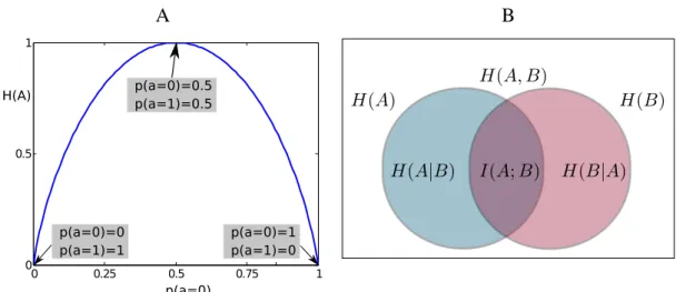
A B 0 0.25 0.5 0.75 1 0 0.5 1 p(a=0) H(A) p(a=0)=0.5_p(a=1)=0.5

p(a=0)=0 p(a=1)=1

p(a=0)=1 p(a=1)=0

Figure 2.3: A: Entropy of the binary variableA∈ {0,1} plotted against p(a=0). It is shown that entropy reaches its maximum value at p(a=0) =p(a=1) =0.5 and its minimum value

at p(a=0) =1 and p(a=0) =0. B: Diagram of the relation between mutual information of

two variablesI(A;B)and their marginal, joint and condition entropies,H(A)andH(B),H(A,B),

H(A|B), respectively.

• H(A)is a concave function of p(a).

The mutual information of two continuous random variablesAandBmeasures the degree of their dependence is defined as follows:

I(A;B) =H(A)−H(A|B) =H(B)−H(B|A) =H(A) +H(B)−H(A,B) = Z A Z B p(a,b)log p(a,b) p(a)p(b)dbda. (2.38)

In other words, mutual information quantifies a change in the uncertainty about one vari-able after the second varivari-able is observed. Note that the entropyH(A) or H(B) can be infinite as da→0 or db→0, respectively. However, the mutual information is always finite because it is defined as a difference of entropies, thus, the infinite terms will vanish [Haykin,1999].

Among the important properties of the mutual information, one can distinguish the fol-lowing:

• the mutual information is symmetric,I(A;B) =I(B;A);

• it is nonnegative, I(A;B)≥0, with equality only if the variablesAandBare inde-pendent.

Conditional mutual information I(A;B|C) measures the amount of information of two variablesAandBconditioned on the variableC:

I(A;B|C) =H(A|C) +H(B|C)−H(A,B|C) = Z A Z B Z C p(a,b,c)log p(a,b|c) p(a|c)p(b|c)dcdbda. (2.39)

Conditional mutual information is a key element of sequential information-theoretical feature selection. Recall that on every iteration we look for a featureF_k that maximizes

I(C;F_k|F_α1, . . . ,F_αi), the mutual information with the class variablesCconditioned on the already selected featuresF_α1, . . . ,F_αi.

Another central concept of information theory is the relative entropy or Kullback-Leibler divergence, which for two probability distributions p(a) and q(a) measures a distance between them: D_KL(p(a)||q(a)) = Z A p(a)logp(a) q(a)da. (2.40)

However, the Kullback-Leibler divergence is not a true metric because it is not symmetric and the triangle inequality does not always hold. Using the definition of the Kullback-Leibler divergence, one can represent the mutual information and get its interpretation in terms of the distance between two distributions:

I(A;B) = Z A Z B p(b)DKL(p(a|b)||p(a))ba. (2.41)

Then, the mutual information measures how much on average the distribution ofAchanges if it is conditioned onB. Obviously, ifAand Bare independent, conditioning onB will not have any effect onAand the average Kullback-Leibler distance will be zero.

For further reading on information theory, refer to [Shannon & Weaver, 1949; Cover &

Thomas,1991;Mackay,2003].

2.4.2

Use in solving classification tasks

Already in 1962 Lewis proposed mutual information between a class variable and a fea-ture as a statistic measuring “goodness” of this feafea-ture for classification [Lewis, 1962]. The statistic had to reflect a degree of correlation between the feature and the class vari-able and it was derived with an objective to reduce a misclassification error. Lewis showed experimentally that the accuracy of the classification was higher when using features with

higher value of the mutual information. Therefore, it was concluded that it is indeed use-ful for selecting features that are relevant for classification. Similar finding appeared also in the field of visual neuroscience, where Ullman and colleagues showed that features maximizing mutual information with a class are optimal for use in visual classification tasks [Ullman et al.,2002].

A more formalized justification for using mutual information as a criterion for selecting discriminative features is based on inequalities relating the Bayes error probability to the conditional entropyp(c|f)and consequently to the mutual informationI(C;F).

For example, the Fano weak lower bound on the conditional entropy [Fano, 1961] states the following:

H(C|F)≤1+p_elog₂(m−1), (2.42)

where p_e is the Bayes error probability when using the feature F for classification and

m is a number of the classes. However, this bound becomes degenerated for two-class problems. Fano also introduced a strong lower bound on this quantity [Fano,1961]:

H(C|F)≤H(p_e) +p_elog₂(m−1). (2.43)

And the upper Hellman-Raviv bound [Hellman & Raviv,1970] is given by the following expression:

H(C|F)≥2p_e. (2.44)

AsI(C;F) =H(C)−H(C|F), it is obvious that a feature F, which maximizes the mu-tual informationI(C;F)or equivalently minimizesH(C|F), assures a small classification error.

Recently Brown and colleagues showed that selection criteria based on mutual informa-tion can be derived from the formulainforma-tion of the condiinforma-tional likelihood maximizainforma