An Efficient Approach to Distributionally Robust Network Capacity Planning

(1)

An Efficient Approach to Distributionally Robust Network

Capacity Planning

Trivikram Dokka1_{, Francis Garuba}1_{, Marc Goerigk}2_{, and Peter Jacko}1 1_{Department of Management Science, Lancaster University, United Kingdom}

2_{Network and Data Science Management, University of Siegen, Germany}

Abstract

In this paper, we consider a network capacity expansion problem in the context of telecommunication networks, where there is uncertainty associated with the expected traf-fic demand. We employ a distributionally robust stochastic optimization (DRSO) frame-work where the ambiguity set of the uncertain demand distribution is constructed using the moments information, the mean and variance. The resulting DRSO problem is formu-lated as a bilevel optimization problem. We develop an efficient solution algorithm for this problem by characterizing the resulting worst-case two-point distribution, which allows us to reformulate the original problem as a convex optimization problem.

In computational experiments the performance of this approach is compared to that of the robust optimization approach with a discrete uncertainty set. The results show that so-lutions from the DRSO model outperform the robust optimization approach on highly risk-averse performance metrics, whereas the robust solution is better on the less risk-risk-averse metric.

Keywords: network design; robust optimization; optimization in telecommunications; distri-butionally robust stochastic optimization

1 Introduction

Uncertainty has been recognized as a reality of our day-to-day living where choices are often made under partial or unknown information. Hence mitigating against uncertainty in decision making has always been a key business driver. In operations research, frameworks have been developed that help to address decision making under uncertainty in two broad areas, namely the stochastic and the robust optimization approaches.

In the stochastic approach, we assign probabilities to the random variables by assuming that the probability distribution of these variables or uncertain data is known or can be accu-rately estimated from historic dataChen et al.(2008). A drawback of this approach is that in real life, the probabilities are often not available or correctly estimated. Robust optimization on the other hand addresses the problem of data uncertainty by assuming that the data lie within

(2)

a closed set Ben-Tal and Nemirovski(1999). It provides an uncertainty immune solution for the worst case of the uncertain data set. Whereas in the robust optimization approach, we op-timize the worst-case objective, in the stochastic optimization approach we opop-timize relevant statistical measures, e.g. expectation, median, CVaR etc. Ignoring the probability information has been a main criticism of the robust approach which may produce an overly conservative solutionChen et al.(2007). Despite the limitations of these two approaches, network design problems under demand uncertainty using these approaches have been frequently considered. Network design has a strategic role within the planning function of most organizations. The task is to ensure the highest quality of design while efficiently balancing the requirement of just enough capacity with the capacity investment cost.Magnanti and Wong(1984);Minoux(1989) provide a survey of the network design models as well as a unifying framework for many of such models. Network design has found application in many areas, such as transportation, supply chain, communications, and social networks.

Thapalia et al.(2012) showed that stochastic just like robust optimization models are often NP-hard, and even the deterministic network design model itself may be difficult to solve for problems of industrial size.Nemirovski et al.(2009) investigated the heuristic methods based on Monte Carlo sampling techniques, stochastic approximation (SA) and sample average ap-proximation (SAA), in their attempt to find a robust stochastic solution. On the other hand,

Bai et al.(2014) compared the result of the deterministic model to the stochastic model using a standard commercial solver while they proposed the use of heuristics or relaxation meth-ods to solve large-scale problems.Sun et al.(2017) determined the quality of the deterministic solutions for a stochastic multi-commodity network design problem and conclude that this so-lution can be used to find a good heuristic soso-lution to the stochastic multi-commodity network design model. The deterministic solution is hence contained in the stochastic solution and us-ing it as a skeleton improves results with as much as 97% of the initial loss recovered. The framework consists of solving a deterministic network design problem, extracting the discrete variables, fixing them in the stochastic model and then solving a stochastic linear problem.

Santoso et al.(2005) solved a supply chain network design problem using sample average approximation and combined this with an accelerated Benders decomposition algorithm to solve a problem with a large number of scenarios. Bidhandi and Yusuff(2011) also study a supply chain network, which was solved using SAA combined with a Benders decomposition algorithm. Kılıc¸ and Tuzkaya(2014) formulate a distribution network as a two-stage design problem and solve this using a MIP methodology called the TSMIP.

Literature abounds on the application of robust optimization to network planning and de-sign following the seminal work of Soyster (1973) and Ben-Tal et al.(1998);Laguna (1998);

Kouvelis and Yu (1997);Ghaoui et al. (1998);Ben-Tal and Nemirovski(1999);Bertsimas and Sim(2003, 2004) among many others. Of particular importance is the work ofBen-Tal et al.

(2004) which introduced the adjustable robust framework that addresses two-stage decision problem where the network planning and design problem is situated. Atamturk and Zhang

(3)

problem which allows the control of the conservatism of the solution via a parameterized bud-get uncertainty set, Ord ´o ˜nez and Zhao (2007) studied the network capacity problem under both demand and travel time uncertainty for a multi-commodity flow problem with single source and sink per commodity whileOuorou and Vial(2007) introduced affine routing con-cept in their robust capacity planning model under demand uncertainty using path-based for-mulation and of recent,Garuba et al.(2019a) addressed non-linearity of cost function in robust network capacity expansion problem. Also, there have been work towards exact solution with

Mattia (2012) being the forerunner while others are Zeng and Zhao (2013); Bertsimas et al.

(2015);Pessoa and Poss(2015);Ayoub and Poss(2016) using different types of decomposition algorithms.

In this paper, to address the drawback of the two approaches, we leverage on their respec-tive strengths and investigate a distributionally robust stochastic stochastic (DRSO) approach to a multi-commodity network design problem, where the probability distribution itself is af-fected by ambiguity. This combination of robust and stochastic optimization for a network capacity planning problem is then analyzed with respect to time of execution, resource usage and applicability in a real world setting

This approach has found increasing application in diverse areas/field since its introduc-tion byScarf(1957) in his min-max solution of inventory problem. Popescu(2007) used this approach in the mean-covariance of the uncertain data distribution to derive a robust solu-tion approach for a max-min and min-max stochastic problem without recourse. Delage and Ye (2010) in their work on distributionally robust stochastic programming develop a model that combines the distribution and moment of the uncertain data. They show that their model outperforms the naive approximated stochastic model proposed byPopescu(2007). However, a polynomial-time algorithm for the larger range of utility functions considered inPopescu

(2007) was beyond the scope of their work. Goh and Sim(2010) on the other hand develop a tractable approximation to a distributionally robust optimization problem. Unlike most min-max stochastic programs, the expectation of recourse variable was included in their model.

Mak et al.(2013) applied the distributionally robust framework to solve an electric vehicle battery swapping station location problem. They also validate the accuracy of this solution against that of the SAA and were able to show that it provides a good approximation to the SAA. Cheng et al. (2016) proposed a new reformulation and approximation for solving the distribution robust shortest path problem building on their earlier work (Cheng et al.,2013). A unifying framework was proposed by Wiesemann et al. (2014) for modeling and solving distributionally robust optimization problems based on standardized ambiguity sets which encompasses many sets from the literature. They identify conditions under which this frame-work is tractable and develop a tractable conservative approximation for problems that violate these conditions.Bertsimas et al.(2018) developed a framework for solving adaptive distribu-tionally robust linear optimization problem.

This paper presents the following contributions: We consider an uncertain network capac-ity expansion problem and develop an efficient algorithm to its distributionally robust

(4)

counter-part by characterizing the resulting two point distribution using Richter-Rogonski’s theorem

Richter(1957);Rogosinski(1958). We compare the quality of solutions from this algorithm to the solutions obtained from a discrete robust approach. It is observed from our numerical ex-periments that solutions found by the DRSO algorithm outperform solutions from the robust optimization approach on highly risk-averse performance metrics.

The model from the literature that is the most similar to ours, but with a flow cost, can be found inNakao et al.(2017). While their approach resulted in a computationally challenging solution approach (including the discretization of continuous values), the model presented here is considerably easier to solve.

The rest of this paper is organized as follows. InSection 2, we describe the general distribu-tionally robust stochastic optimization concept. Section 3explains the robust network design problem we consider. In Section 4, our efficient formulation of the distributionally robust problem is developed. We first focus on the single-commodity case and then extend results to the multi-commodity case. InSection 5, the experimental setup and computational result are discussed. Finally,Section 6concludes our work and points out future research directions.

2 Distributionally Robust Stochastic Optimization

Distributionally robust stochastic optimization is a data-driven modeling methodology for optimization under uncertainty. It encompasses aspects from both robust and stochastic op-timization, frameworks that are complementary to each other though differing in their ap-proaches to addressing the uncertaintyBen-Tal et al.(2009).

Robust optimization provides a framework to immunize against uncertainty that is be-lieved to lie within a closed and bounded set known as the uncertainty set, while the stochastic optimization framework assumes that the probability distribution of these parameter uncer-tainty is known. However, in real world application, ”true” distribution knowledge is never completely known but at most can only be estimated from available data Shapiro and Kley-wegt (2002). On the other hand, one of the major attractiveness which has resulted in the explosion of research into the robust framework is its tractability to a wide range of challeng-ing problems. Nevertheless, this methodology also faced criticism for its inability to factor in the distribution knowledge of the underlying uncertain data, leading to overly conservative solutionsWiesemann et al.(2014);Chen et al.(2007).

Uncertainty can be viewed asriskwhen the probability distribution is known or as an ambi-guityotherwiseBertsimas et al.(2018). Neither of these two approaches is suitable to deal with ambiguity from the perspective of decision theory. However, combining the uncertainty set of the robust approach with the probability distribution from the stochastic approach produces a more potent methodology that is able to handle both risk and ambiguity. Hence, under the distributionally robust stochastic framework, the probability distribution is also subjected to uncertainty. The aim is to find a decision such that for any possible probability distribution from the ambiguity set, the stochastic constraints of the model are satisfied.

(5)

In the era of growing data-driven applications, moments that constitute the ambiguity are estimated in the face of limited historical data.Scarf(1957) was the first to apply this methodol-ogy in his min-max proposal to the newsvendor problem where the ”true” distribution, though not known completely, is only characterized by its mean and standard deviation and belongs to a class of probability distributions with the same mean and standard deviation. The distri-butionally robust stochastic approach hence seeks to maximize the expectation by considering the worst case distribution in this probability distributions class also known as the ambiguity set.

3 Problem Description

Planning for capacities to be added in networks is a major strategic problem in most telecom-munication organizations. Usually, this decision is made under uncertainty of the future traffic demand. As with most strategic roles, this often involves large capital expenditure investment. Hence, in this paper, we consider a multi-commodity network demand flow problem, where additional capacities are added to accommodate uncertain traffic demands while minimizing the total cost involved subject to design constraints.

3.1 Basic Network Expansion Problem

The problem can be represented by a directed graph G = (V,A)which denotes the network of interest. Each of the arcsa∈ Ahas an original capacityuawhich can be upgraded at a cost ca per incremental unit of capacity. A set of commoditiesK = {1, . . . , K} need to be routed

across the network with each commodityk∈ Kconsisting of a demanddk ≥0, a source node

sk ∈ V, and a sink nodetk ∈ V. Additionally, letφbe the cost of not satisfying one unit of demand over the planning horizon (i.e., by outsourcing it). Under complete demand certainty, the nominal network capacity expansion problem can then be formulated as:

min X a∈A caxa+φ X k∈K  dk− X a∈δ−₍_tk₎ f_ak+ X a∈δ+₍_tk₎ f_ak   + (1) s.t. X a∈δ−₍_v₎ f_ak− X a∈δ+₍_v₎ f_ak≥0 ∀k∈ K, d∈ U, v ∈ V \ {sk, tk} (2) X k∈K f_ak≤ua+xa ∀a∈ A (3) f_ak ≥0 ∀k∈ K, d∈ U, a∈ A (4) xa≥0 ∀a∈ A (5)

Here,[y]+denotes the positive partmax{0, y}, whileδ+(v)andδ−(v)are the sets of the outgo-ing and incomoutgo-ing arc at nodev ∈ V, respectively. Variablesf_ak denote the flow of commodity

k ∈ K along edgea ∈ A, whilexamodels the amount of capacity being added to arca. The

(6)

Constraints (2) are a variant of flow constraints, where we allow an arbitrary amount of flow to leave the source nodesk. Through the objective, only the flow arriving intkis counted. Finally, Constraints (3) which model the capacity on each edge ensure that amount of flow does not exceed the sum of initial and added capacity.

3.2 Robust Problem Formulation

Since the actual demand valuesddd = (d1, . . . , dK) ∈ RK+ are uncertain, we assume here that they can take any value in a predetermined uncertainty set U, which can be represented as U = {ddd1, . . . , dddN}. The network capacity expansion problem using the robust optimization framework is to minimize the cost of capacity investment and the worst-case costs of out-sourced (unsatisfied) demand while satisfying the network constraints. The robust network design for uncertainty setU is hence:

min X a∈A caxa+ max ddd∈U φ X k∈K  dk− X a∈δ−₍_tk₎ f_ak(ddd) + X a∈δ+₍_tk₎ f_ak(ddd)   + (6) s.t. X a∈δ−₍_v₎ f_ak(ddd)− X a∈δ+₍_v₎ f_ak(ddd)≥0 ∀k∈ K, ddd∈ U, v ∈ V \ {sk, tk} (7) X k∈K f_ak(ddd)≤ua+xa ∀ddd∈ U, a∈ A (8) f_ak(ddd)≥0 ∀k∈ K, ddd∈ U, a∈ A (9) xa≥0 ∀a∈ A (10)

with a scenariodddbeing the demand vector over all commodities. As before,φis a penalty pa-rameter for uncovered demand (e.g., outsourcing costs). We can send as much flow as we like, but flow cannot appear outside the source, and sending insufficient flow creates a penalty. The constraints (1)-(5) have been updated to take uncertainty into account, hence the worst case is considered in constraints (6). The positive part[·]+ in the objective can be easily linearized using additional variablesτk≥0and constraintsτk≥dk−P

a∈δ−₍_tk₎f_ak(ddd) + P

a∈δ+₍_tk₎f_ak(ddd) for allk∈ K. The inner maximum can be linearized in an analogous way.

4 Distributionally Robust Stochastic Problem Formulation

4.1 Single-Commodity Case

The single commodity network design problem with outsourcing can be modeled as below. Notice that we drop the subscriptkfromdk,skandtk, because we assume a single commodity

(7)

problem, i.e.,K = 1; min X a∈A caxa+φmax P∈P EP d−d˜₊ (11) s.t. X a∈δ−₍_v₎ fa− X a∈δ+₍_v₎ fa = 0 ∀v∈ V\{s, t} (12) X a∈δ−₍_t₎ fa− X a∈δ+₍_t₎ fa= ˜d (13) X a∈δ−₍_s₎ fa− X a∈δ+₍_s₎ fa=−d˜ (14) fa≤ua+xa ∀a∈ A (15) fa≥0 ∀a∈ A (16) ˜ d≥0 (17) xa≥0 ∀a∈ A (18)

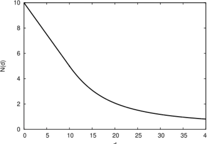
In this formulation,d˜is the amount of demand that we intend to satisfy. We consider the prob-lem as a bilevel optimization probprob-lem, where first the network owner makes his decision of the amount of demand he wishes to satisfy, and then nature chooses a probability distribution for the demand which maximizes the expected unsatisfied demand. So the second level problem (nature’s problem) is max P EP d−d˜₊ (19) s.t. EP d =µ (20) EP d−µ2 =σ2 (21)

This means we consider all probability distributionsPoverdthat have the same meanµand varianceσ2. We denote this set asP. We can thus rewrite the DRSO problem as

min (xxx,fff ,d˜)∈X

X

a∈A

caxa+φN( ˜d)

whereN( ˜d)denotes the value of the inner nature’s problem, andXthe set of feasible solutions with respect toxxx,fffandd˜.

4.2 Model Reformulation

Lemma 1 Let some first-stage solution(xxx, fff ,d˜)be fixed. The optimal objective value of nature’s prob-lem can then be written as

N( ˜d) =      1/2 µ−d˜+ q ( ˜d−µ)2₊_σ2 ifd >˜ µ2₂+_µσ2 µ−d˜_µ2µ₊2_σ2 ifd˜≤ µ2₊_σ2 2µ (22)

(8)

Proof:A proof of the result can be found in Lo(1987) . Recall thatN( ˜d) = max_P∈PEP[max(d− ˜

d,0)]. It can be shown that there is a worst-case distribution that is a two-point distribution, which follows from the Richter-Rogonski theoremRichter(1957);Rogosinski(1958). For the

sake of completeness, we present a proof in AppendixA.

An example for the shape of functionN( ˜d)is presented inFigure 1.

0 2 4 6 8 10 0 5 10 15 20 25 30 35 40 N(d) d

Figure 1: Example shape ofN( ˜d)withµ= 10andσ2= 100. In this case,(µ2+σ2)/2µ= 10.

Lemma 2 The functionN( ˜d)is convex.

Proof:The first derivative ofN with respect tod˜is

∂N ∂d˜ =      1 2 ˜ d−µ √ ( ˜d−µ)2₊_σ2 −1 ifd >˜ µ2₂+_µσ2 −_µ2µ₊2_σ2 ifd˜≤ µ2₊_σ2 2µ

and the second derivative is

∂2N ∂d˜2 =    σ2 2(( ˜d−µ)2₊_σ2₎32 if ˜ d > µ2₂+_µσ2 0 ifd˜≤ µ2₂+_µσ2

Note that the first derivative is continuous, as 1 2   µ2+σ2 2µ −µ q (µ2₂+_µσ2 −µ)2₊_σ2 −1  = 1 2   σ2−µ2 2µ q (µ2₂+_µσ2)2₋₍_µ2₊_σ2_{) +}_µ2₊_σ2 −1   = 1 2   σ2₋_µ2 2µ q (µ2₂+_µσ2)2 −1  = 1 2   σ2₋_µ2 2µ µ2₊_σ2 2µ −1  = 1 2 σ2−µ2 µ2₊_σ2 −1 = 1 2 − 2µ 2 µ2₊_σ2 =− µ 2 µ2₊_σ2,

and it is non-decreasing. Hence, the function is convex.

(9)

problem for fixed value ofd˜. Then, F( ˜d) = min (xxx,fff)∈X( ˜d) X a∈A caxa+φN( ˜d)

where as before,N( ˜d)is the objective of the adversary problem, andX( ˜d)is the set of vectors

xxxandfff that give a flow valued˜. We rewrite this to

F( ˜d) =φN( ˜d) +G( ˜d) whereG( ˜d) = min₍_x_x_x,f_f_f₎_∈_X_{( ˜}_d₎P

a∈Acaxa. Theorem 1 The functionF( ˜d)is convex.

Proof: We show thatG( ˜d)is a convex function ind˜. This, together with the fact thatN( ˜d)is convex due to Lemma2, implies that their sum,F( ˜d)is also convex.

Consider the functionG0( ˜d), where

G0( ˜d) = min X a∈A caxa+ψ· ˜ d− X a∈δ−₍_t₎ fa+ X a∈δ+₍_t₎ fa (23) s.t. X a∈δ−₍_v₎ fa− X a∈δ+₍_v₎ fa = 0 ∀v∈ V\{s, t} (24) fa≤ua+xa ∀a∈ A (25) fa≥0 ∀a∈ A (26) xa≥0 ∀a∈ A (27)

for a large value ψ ≥ P

a∈Aca. Let (xxx0, fff0)be an optimal solution to G0( ˜d) and assume that

∆ := |d˜−P

a∈δ−₍_t₎f_a0 +P_a_∈_δ+₍_t₎f_a0| > 0. Then we can increase eachx0_aby ∆to find a new solution where there is sufficient capacity to outsource no demand at all. As increasing the capacity this way increases the costs by∆P

a∈Acaandψ >P_a∈Aca, we have constructed a

new solution that is feasible and has no higher objective value that(xxx0, fff0). Hence there is an optimal solution toG0( ˜d)that meet exactly a demand ofd˜. Therefore,G0( ˜d) =G( ˜d).

Recall that if a functionf1(x, y)is convex in(x, y)andCis a convex set, then

f2(x) = inf

y∈Cf1(x, y)

is convex as wellBoyd and Vandenberghe(2004). Therefore,G( ˜d) =G0( ˜d) = min₍_x,f_x_x_f_{f ,}_d˜₎_∈_XP_a∈Acaxa+ ψ· |d˜−P

a∈δ−₍_t₎f_a+P_a_∈_δ+₍_t₎fa|withXrepresented by constraints (24-27) is convex.

We can useTheorem 1to solve the single-commodity DRSO problem efficiently. For a fixed valued˜, we evaluate F( ˜d)by solving G( ˜d) as a linear program andN( ˜d) using the formula provided in Equation 22. We can now apply standard convex optimization methods (in our experiments we use the Nelder-Mead method) to solvemin_d˜F( ˜d)to optimality.

(10)

4.3 Extension to the Multi-Commodity Case

In this setting, we assume that the demand at each of the origin-destination pairs (sk, tk) is affected by a different distribution. In particular, we have meanµk and varianceσk2 for each k∈ K. The nature problem in this case becomes:

max EP " X k∈K [dk−d˜k]+ # (28) s.t. EP dk=µk ∀k∈ K (29) EP dk−µk 2 =σ_k2 ∀k∈ K (30)

The DRSO problem can now be written as

min X a∈A caxa+φ·N(˜ddd) (31) s.t. X a∈δ−₍_v₎ f_ak− X a∈δ+₍_v₎ f_ak= 0 ∀k∈ K, v∈ V\{sk, tk} (32) X a∈δ−₍_tk₎ f_ak− X a∈δ+₍_tk₎ f_ak = ˜dk ∀k∈ K (33) X a∈δ−₍_sk₎ f_ak− X a∈δ+₍_sk₎ f_ak=−d˜k ∀k∈ K (34) f_ak≤ua+xa ∀k∈ K, a∈ A (35) f_ak≥0 ∀k∈ K, a∈ A (36) xa≥0 ∀a∈ A (37)

where N(˜ddd) denotes the multi-dimensional version of nature’s problem as defined by equa-tions (28)-(30).

Corollary 2 The optimal solution for nature’s problem defined by equations(28)-(30)can be expressed as

N(˜ddd) =X

k∈K

N( ˜dk) (38)

Proof: This extends Lemma1using the linearity of the expectation on the one hand, and the decomposability of nature’s problem on the other hand. We have

N(˜ddd) = max P∈P EP " X k∈K [dk−d˜k]+ # = max P∈P X k∈K EP h [dk−d˜k]+ i =X k∈K max P∈P EP h [dk−d˜k]+ i =X k∈K N( ˜dk)

(11)

Moreover, it can be easily verified thatN( ˜ddd˜˜)is convex, as it is a sum of convex functions.

5 Experiments

5.1 Setup

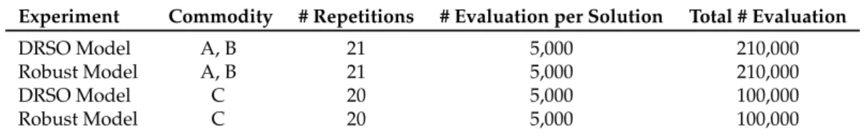
Our models were implemented using a real-world network from the SNDLib library (see Or-lowski et al.(2010)), the Nobel-US network with 14 nodes and 42 arcs. A sample of 10,000 demand scenarios was generated to form our reference set, sampling i.i.d from a gamma dis-tribution with shape4and scale5while discarding negative demands and any demand above 50. Three instances of20source-sink node pairs were randomly generated for the test network; commodity set A, commodity set B and commodity set C. We then sample training sets for the optimization models. Commodities A and B use the same set of 60 scenarios. For commodity C, we sample a separate set of 60 scenarios. These are used as discrete uncertainty sets for the robust model, and to compute the empirical mean and the variance for the DRSO model.

The solutions found by the two optimization models are then evaluated with demands from the reference set using 5,000 scenarios. The whole experimental setup is repeated 21 times for commodities A and B, and 20 times for commodity C. We provide an overview on the experimental setup inTable 1.

The cost of capacity allocation to the arc is randomly generated using a normal distribution with mean40and variance36, while the penalty of unsatisfied or outsourced demand was set to 130 using10(N −1), whereN is the number of arcs.

Table 1: Experimental setup.

Experiment Commodity # Repetitions # Evaluation per Solution Total # Evaluation

DRSO Model A, B 21 5,000 210,000

Robust Model A, B 21 5,000 210,000

DRSO Model C 20 5,000 100,000

Robust Model C 20 5,000 100,000

The results of the two models are recorded as the in-sample results where the first-stage investment cost of the objective value (Cap. Inv) is the cost of deploying capacity and O/S demand is the outsourced (unsatisfied) demand, which when multiplied by the unit penalty cost (φ) gives the second-stage outsourcing costs of the objective value. The performance of the evaluation model is reported in terms of mean outsourced demand (E[O/S]), expected maximum outsourced demand(E[max O/S]), average outsourced demand over the worst 5% values (CVaR95), average outsourced demand over the worst 25% values (CVaR75) and the mean satisfied demand E[d˜]. The first of these metrics, the E[O/S], is a low risk measure while the rest three are high risk measures. The two models were implemented using Julia and Gurobi version 7.5 on a Lenovo desktop machine with 8GB RAM and Intel Core i5-65 CPU with 2.50GHz using Windows 10 (64-bit) OS.

(12)

using the below model. This seeks to calculate an optimal flow for a fixed scenariodddwhile minimizing the expected outsourced demand τk in each commodity k ∈ K, due to lack of adequate capacity. As the first-stage investment is already fixed, we fix thexxxsolution in this model. min X k∈K τk s.t. X a∈δ−₍_v₎ f_ak− X a∈δ+₍_v₎ f_ak= 0 ∀k∈ K, v∈ V\{sk, tk} X a∈δ−₍_tk₎ f_ak− X a∈δ+₍_tk₎ f_ak = ˜dk ∀k∈ K X a∈δ−₍_sk₎ f_ak− X a∈δ+₍_sk₎ f_ak=−d˜k ∀k∈ K τk≥dk−d˜k ∀k∈ K f_ak≤ua+xa ∀k∈ K, a∈ A f_ak≥0 ∀k∈ K, a∈ A ˜ dk≥0 ∀k∈ K τk≥0 ∀k∈ K

For each xxx solution, 5,000 evaluations are done and the outsourced demand together with satisfied demand are recorded for each evaluation.

5.2 Computational Results

Table 2presents a high level summary of the experimental results. Recall that three instances of20S-T pairs were used, which are denoted as commodities A, B and C in the table. Each row of results under commodities A and B in the table is the average of21instances while the ones under commodity C is the average of20 instances of different60demand samples. The first three columns results are the in-sample optimization result while the next two are the out-of-sample evaluation result. The average (E[O/S]), the maximum (E[Max O/S]), average of the largest5%(CVaR95) and average of largest25%(CVaR75) are calculated from the5,000 eval-uation results for the outsourced demand as the out-of-sample results. While for the satisfied demand, only the average (E[d˜]) is calculated.

In the following, we focus on the evaluation for commodity type A. Results for commodity types B and C can be found in AppendixBand AppendixC, respectively.

FromTable 2, it is observed that DRSO solutions build less capacity compared to the robust solutions for all demand instances and hence a lower capital investment, both in terms of total investment and capacity investment. The capacity investment is the cost of adding capacity, the first term of the objective function, while the total investment is the objective value of the optimization problem. The observation seems valid irrespective of the commodity and data set used. For commodity A, the robust solution builds approximately74%more capacity than the

(13)

Table 2: Comparing the two models under two commodities.

Commodity A Tot. Inv Cap. Inv O/S Dem E[O/S] E[d˜] Cap Add Unit Cost

Robust 44,679.05 32,641.54 92.60 70.91 372.02 842.09 38.76 DRSO 41,830.77 18.671.69 178.15 159.75 267.28 484.99 38.50 Commodity B Robust 43,548.63 28,685.06 114.33 86.22 355.32 730.25 39.29 DRSO 41,081.28 19,255.14 167.89 150.49 280.37 489.35 39.35 Commodity C Robust 50,878.38 29,226.48 166.55 132.37 281.68 705.39 41.43 DRSO 47,290.23 11,734.21 273.51 261.79 141.53 283.55 41.38

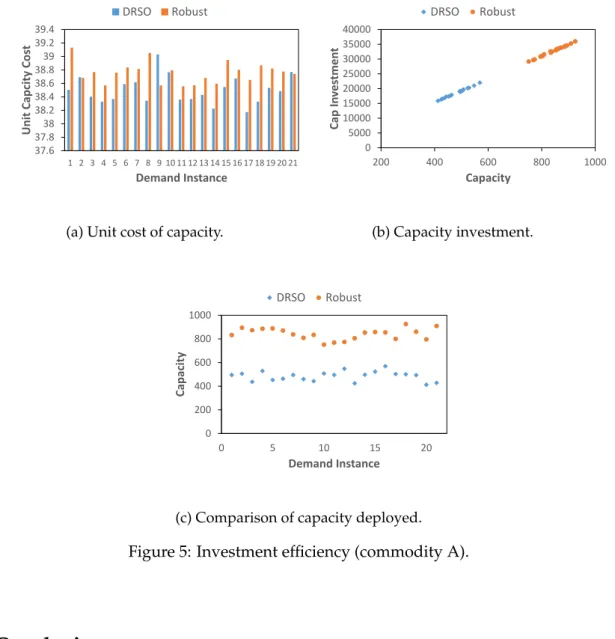
DRSO solution (50%and150%more in case of commodity B and C, respectively). Though this result is the average over all demand instances, it is also true for each single demand instance, seeFigure 5c.

Table 3: Robust model results for commodity type A.

In Sample Out of Sample

Inst. Cap. Inv. O/S Demand E[O/S] E[Max O/S] CVaR95 CVaR75 E[d˜] CapAdd

1 32,589.64 97.48 72.91 562.76 407.99 231.40 378.76 832.84 2 34,600.41 77.58 59.55 525.62 369.93 199.51 385.59 894.49 3 33,855.56 78.89 65.59 558.41 402.72 219.72 375.00 873.30 4 34,166.13 75.71 60.50 525.91 378.00 204.94 376.94 885.85 5 34,445.25 88.87 64.67 545.86 391.37 215.37 370.99 888.71 6 33,818.93 90.58 65.47 542.46 387.26 215.31 387.39 870.78 7 32,527.15 95.14 75.24 561.43 411.77 239.97 364.20 838.04 8 31,603.34 106.24 74.96 561.52 407.47 232.43 372.81 809.27 9 32,173.50 103.65 77.82 561.57 405.88 231.07 370.11 834.15 10 29,153.00 99.19 91.97 585.70 437.79 264.62 355.20 751.48 11 29,642.85 118.30 82.57 578.90 423.41 250.96 350.37 768.80 12 29,848.79 124.09 86.77 579.68 423.98 245.93 354.20 773.85 13 31,146.65 106.54 75.19 561.82 410.03 239.60 363.83 805.23 14 32,925.94 80.73 67.86 551.43 396.82 222.27 363.21 853.06 15 33,431.34 90.17 67.58 555.29 403.51 228.90 374.53 858.36 16 33,160.00 90.34 68.89 544.42 390.52 216.68 369.76 854.61 17 30,910.42 93.55 75.41 579.02 424.54 246.26 352.29 799.72 18 35,969.65 74.46 52.75 524.08 368.39 190.02 395.79 925.42 19 33,415.01 84.78 67.08 540.52 387.26 212.55 384.07 860.78 20 30,853.02 93.20 78.69 574.63 425.13 248.80 358.67 795.68 21 35,235.78 75.03 57.68 515.23 363.10 200.72 408.72 909.52

Table 3andTable 4present the results for each demand instance for the robust and DRSO solutions respectively. For the same demand instance, the DRSO solution invests less in capac-ity, which can be expected since it takes the distribution information of the random variable into consideration unlike the robust model. The DRSO solution is less conservative in this re-gards, whereas the robust solution plans for the worst observed realization of the random vari-able. The DRSO solution is therefore cost efficient, building only the needed capacity based on the distribution information which lowers the investment cost, while the robust solution seems to take the more pessimistic route. Comparing each demand instance, the penalty cost

(14)

Table 4: DRSO model results for commodity type A.

Inst. Cap. Inv. Nature d˜ E[O/S] E[ Max O/S] CVaR95 CVaR75 E[d˜] CapAdd

1 19,066.17 176.23 300.70 154.02 698.87 543.18 356.25 278.11 495.16 2 19,577.97 171.08 297.69 150.88 688.22 532.53 350.41 279.93 506.00 3 16,785.07 185.68 267.71 173.22 726.25 570.56 383.89 254.52 437.08 4 20,276.51 162.84 307.05 142.09 677.09 521.40 339.98 286.83 529.02 5 17,372.72 192.30 271.26 176.06 728.31 572.62 385.63 246.74 452.77 6 17,882.24 183.66 283.42 168.07 716.15 560.46 373.48 261.94 463.40 7 19,125.03 170.55 292.95 154.98 704.27 548.58 361.60 271.78 495.25 8 17,633.05 197.36 275.90 169.89 717.59 561.90 376.29 258.67 459.89 9 17,282.82 195.63 261.69 180.33 737.88 582.19 395.31 237.93 442.80 10 19,688.38 161.49 292.87 151.62 700.52 544.83 359.57 274.50 507.90 11 19,001.74 172.63 298.09 152.80 697.06 541.37 354.93 274.36 495.37 12 21,012.66 162.36 317.59 136.45 670.18 514.49 332.53 292.79 547.64 13 16,316.88 202.74 264.19 184.32 735.38 579.69 392.82 246.14 424.59 14 18,998.62 172.22 291.80 152.49 704.37 548.68 361.77 268.54 497.03 15 20,174.18 166.03 304.22 144.64 695.35 539.66 352.67 282.83 523.39 16 22,007.06 144.70 318.79 132.10 680.78 525.08 338.10 298.47 569.06 17 19,207.57 172.70 296.34 151.61 700.80 545.11 358.26 269.02 503.15 18 19,184.25 176.21 292.80 156.95 706.77 551.08 364.10 261.23 500.53 19 19,023.42 173.25 296.49 153.29 688.88 533.19 352.03 276.72 493.69 20 15,879.57 198.35 257.87 185.17 741.70 586.01 399.03 243.59 412.61 21 16,609.68 203.07 260.61 183.82 738.96 583.26 396.28 248.14 428.43

of outsourced demand is lower for the robust solution, which is attributed to the fact that it builds for the worst case.

Evaluating the performance of the optimization solution, which is reported by the out-sample performance in Table 3 andTable 4, the expected unsatisfied demand and expected satisfied demand are lower compared to the DRSO solution. All other high-risk metrics are higher for the DRSO solution. The first four metrics are derived from the expected unsatisfied demand which explains this observation while the satisfied demand on the other hand is a function of the capacity already installed for which the DRSO solution is less conservative. However, this simple comparison may not fully explain the performance of the models, hence we will rely on the charts presented inFigure 2to Figure 5. The capacity investment, on the horizontal axis, is compared with the four expected unsatisfied demand metrics inFigure 2a

toFigure 2d.

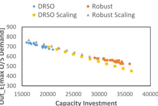
Each of these four charts gives the same observation: Solutions based on the robust model,at higher investment cost, are revealed to be generally more robust than solutions based on DRSO model, which are at lower investment region. For an unexpected surge in traffic, the solution based on robust model will be more able to accommodate this surge compared to the DRSO solution, as its expected outsourced demand is lower. However, in order to allow for a fair comparison of these two models and to be sure this observation is consistent for both models in all the investment regions, we scale a robust solution up towards the DRSO solutions area while scaling down a DRSO solution towards the robust solutions area using expected unsat-isfied demand that is presented inFigure 2a. This scaling, which was also used inGaruba et al.

(15)

0 50 100 150 200 10000 20000 30000 40000 Out _ E[O/ S Demand] Capacity Investment DRSO Robust

(a) Expected unsatisfied demand.

300 400 500 600 700 800 15000 20000 25000 30000 35000 40000 Out _ E[ma x O/ S Demand] Capacity Investment DRSO Robust

(b) Expected maximum unsatisfied demand.

200 250 300 350 400 450 500 550 600 650 10000 20000 30000 40000 Out _ E[CV aR95 Deman d] Capacity Investment DRSO Robust

(c) CVaR95 unsatisfied demand.

0 50 100 150 200 250 300 350 400 450 10000 20000 30000 40000 Out _ E[Cv aR75 Deman d] Capacity Investment DRSO Robust

(d) CVaR75 unsatisfied demand.

Figure 2: Expected unsatisfied demand mean and risk measures (commodity A).

(2019b), is carried out using a representative data point for each model. We scale thexxxsolution in the direction of interest and re-evaluate with the out-of-sample set. In personal experience, this is also common in the industry, where an optimal solution is scaled up or down during planning iteration, thus allowing for a comprehensive comparison of the two models in all the investment regions. The DRSOxxxsolution is multiplied by a factor ofλ= 1.0toλ= 1.8, where

λis the scaling factor, with a scale interval of0.08, to scale up the solution towards the high investment area while the robust solution is multiplied by a factor ofλ= 1.0toλ= 0.5, with a scale interval of0.05, to scale down the solution towards the low investment area. The result of this scaling is as shown inFigure 3which to the contrary shows that for highly risk-averse metrics (maximum and CVaRs of expected unsatisfied demand), solutions based on the DRSO model are in fact better, having a higher degree of robustness with increasing capacity invest-ment even for high investinvest-ment. However, for the less risk-averse metric (expected unsatisfied demand), the robust model gives a better solution at higher investment region but with com-parable performance for lower investment cost. This observation is consistent for the other two commodities B and C, seeFigure 7andFigure 10in the appendix.

(16)

0 50 100 150 200 250 10000 20000 30000 40000 Out _ E[O/ S Demand] Capacity Investment DRSO Robust

DRSO Scaling Robust Scaling

300 400 500 600 700 800 900 15000 20000 25000 30000 35000 40000 Out _ E[ma x O/S Demand ] Capacity Investment DRSO Robust

200 300 400 500 600 700 10000 20000 30000 40000 Out _ E[CV aR95 Deman d] Capacity Investment DRSO Robust

(c) CVaR95 unsatisfied demand

0 100 200 300 400 500 10000 15000 20000 25000 30000 35000 40000 Out _ E[Cv aR75 Deman d] Capacity Investment DRSO Robust

Figure 3: Performance metric scaling (commodity A).

Next we compare the unsatisfied demand (in-sample) to the expected outsourced demand (out-of-sample) for these two models to see which of these gives a better estimate. The charts inFigure 4atoFigure 4epresent these results and they show that the DRSO results produce a far better estimate and hence a better predictor of the input variables under data uncertainty. On the average the input/output ratio of the unsatisfied demand (in-sample) to the expected unsatisfied demand (out-of-sample) is around 10.3% (commodities B and C respectively are 10.3%and4.29%) for the DRSO model, while for the robust model, this is as high as23.43% (commodities B and C respectively are24.59%and20.52%). Also, regression analysis in Fig-ure 4ashows that 93% variation in the estimate is explained by the in-sample result for the DRSO model while for the robust model this is approximately71%, seeFigure 4b. The result follows the same pattern for the maximum expected unsatisfied demand with respect to the unsatisfied demand in Figure 4c for DRSO with R2 _{= 0}_.₈₁₂₁ _and _{Figure 4d} _{for the robust} model withR2 = 0.6048.

A similar trend is also observed for the satisfied demand (d˜) metric with an I/O gap of 7.35%(commodities B and C respectively are7.23%and4.20%) while the regression result in

(17)

y = 0.9892x - 16.461 R² = 0.9252 50 70 90 110 130 150 170 190 210 120 140 160 180 200 220 Out of Samp le In Sample E_O/S

(a) DRSO solutions, expected demand gap.

y = 0.5935x + 15.956 R² = 0.7055 20 30 40 50 60 70 80 90 100 50 70 90 110 130 Out of Samp le In Sample E-O/S

(b) Robust solutions, expected demand gap.

y = 1.2277x + 488.68 R² = 0.8121 620 640 660 680 700 720 740 760 120 140 160 180 200 220 Out of Samp le In Sample Max E_O/S

(c) DRSO solutions, expected max demand gap. y = 1.1385x + 448.68 R² = 0.6048 500 520 540 560 580 600 50 70 90 110 130 Out of Samp le In Sample Max E_O/S

(d) Robust solutions, expected max demand gap. y = 0.8875x + 11.591 R² = 0.941 210 230 250 270 290 310 220 240 260 280 300 320 340 Out of Samp le In Sample E_d-tilde

(e) DRSO solutions, expected satisfied de-mand gap.

Figure 4: Results of out-of-sample prediction (commodity A).

Figure 4eshows that94.10%(commodities B and C respectively are94.78%and98.83%) varia-tion in the expected satisfied demand (E[d˜]) is explained by the in-sample result, which means that 5.90% variation in the expected satisfied demand is not due to the in-sample satisfied

(18)

demand.

Although the robust solutions follow a pessimistic route and build more capacity for the same demand instances, there is no observed significant difference in the average unit cost of capacity for these two models irrespective of commodity type and data set, seeTable 2. For commodity A, for instance, with average unit capacity cost of 38.50 for the DRSO solutions and38.76for the robust solutions.

Additional insight on this is provided by Figure 5a, which compares the unit cost per in-stance and byFigure 5b, which shows similar linear relationship between capacity and invest-ment for the two models. However, if the capacity installed is compared to the total investinvest-ment cost, the unit cost of robust solutions becomes cheaper.

37.6 37.8 38 38.2 38.4 38.6 38.8 39 39.2 39.4 1 2 3 4 5 6 7 8 9 10 11 12 13 14 15 16 17 18 19 20 21 Unit Capcity Cos t Demand Instance DRSO Robust

(a) Unit cost of capacity.

0 5000 10000 15000 20000 25000 30000 35000 40000 200 400 600 800 1000 Cap In v es tmen t Capacity DRSO Robust (b) Capacity investment. 0 200 400 600 800 1000 0 5 10 15 20 Capacity Demand Instance DRSO Robust

(c) Comparison of capacity deployed.

Figure 5: Investment efficiency (commodity A).

6 Conclusions

In this paper an efficient approach to distributionally robust network capacity planning un-der demand ambiguity was proposed. In this approach, we formulate the problem as bilevel

(19)

optimization, where the worst-case distribution can be characterized by a two-point distribu-tion. This allows us to reformulate the problem as a convex optimization problem, where we need to search over the demanddd˜dwe intent to satisfy. We then solve this new model using Nelder-Mead algorithm, a convex optimization method.

In order to evaluate the quality of our new approach, the resulting model was compared with the robust approach model on the Nobel-US network taken from the SNDlib,Orlowski et al.(2010), database on a number of performance metrics. Our computational result show that solutions from the DRSO model outperform those from the robust model on all high risk-averse performance metrics. Even in the area of solution robustness and quality where the later is generally of a higher robustness, the result scaling shows that solutions from DRSO outperform the robust model in this area on the high risk measures. The robust, however, performs better on the low risk-averse metric.

One interesting result which was also reported earlier by Nakao et al.(2017) using a dif-ferent metric is the prediction accuracy of the DRSO model with over 90% expected result variability explained by model result whereas the Robust model cannot be relied upon hav-ing a prediction accuracy of approximately57%and higher. It was also noted that despite the performance difference, the actual unit cost of capacity for this two model is not significantly different.

Moreover, the solutions based on the DRSO were found to be less conservative when com-pared to Robust model, irrespective of the observed demand instance, data set used and the commodity type, with lower total and capacity investment.

References

Atamturk, A. and Zhang, M. (2007). Two-stage robust network flow and design under demand uncertainty. Operations Research, 55(4):662–673.

Ayoub, J. and Poss, M. (2016). Decomposition for adjustable robust linear optimization subject to uncertainty polytope. Computational Management Science, 13(2):219–239.

Bai, R., Wallace, S. W., Li, J., and Chong, A. Y.-L. (2014). Stochastic service network design with rerouting. Transportation Research Part B: Methodological, 60:50–65.

Ben-Tal, A., El Ghaoui, L., and Nemirovski, A. (1998). Robust semidefinite programming. Handbook on Semidefinite Programming, 27.

Ben-Tal, A., El Ghaoui, L., and Nemirovski, A. (2009). Robust Optimization. Princeton Univer-sity Press.

Ben-Tal, A., Goryashko, A., Guslitzer, E., and Nemirovski, A. (2004). Adjustable robust solu-tions of uncertain linear programs. Mathematical Programming, 99(2):351–376.

Ben-Tal, A. and Nemirovski, A. (1999). Robust solutions of uncertain linear programs. Opera-tions Research Letters, 25(1):1–13.

(20)

Bertsimas, D., Dunning, I., and Lubin, M. (2015). Reformulation versus cutting-planes for robust optimization. Computational Management Science, 13(2):195–217.

Bertsimas, D. and Sim, M. (2003). Robust discrete optimization and network flows. Mathemat-ical Programming, 98(1-3):49–71.

Bertsimas, D. and Sim, M. (2004). The price of robustness. Operations Research, 52(1):35–53. Bertsimas, D., Sim, M., and Zhang, M. (2018). Adaptive distributionally robust optimization.

Management Science, 65(2):604–618.

Bidhandi, H. M. and Yusuff, R. M. (2011). Integrated supply chain planning under uncertainty using an improved stochastic approach. Applied Mathematical Modelling, 35(6):2618–2630. Boyd, S. and Vandenberghe, L. (2004). Convex optimization. Cambridge university press. Chen, X., Sim, M., and Sun, P. (2007). A robust optimization perspective of stochastic

program-ming. Operations Research, 55(6):1058–1071.

Chen, X., Sim, M., Sun, P., and Zhang, J. (2008). A linear decision-based approximation ap-proach to stochastic programming. Operations Research, 56(2):344–357.

Cheng, J., Leung, J., and Lisser, A. (2016). New reformulations of distributionally robust short-est path problem. Computers & Operations Research, 74:196–204.

Cheng, J., Lisser, A., and Letournel, M. (2013). Distributionally robust stochastic shortest path problem. Electronic Notes in Discrete Mathematics, 41:511–518.

Delage, E. and Ye, Y. (2010). Distributionally robust optimization under moment uncertainty with application to data-driven problems. Operations Research, 58(3):595–612.

Garuba, F., Goerigk, M., and Jacko, P. (2019a). Robust network capacity expansion with non-linear costs. In Cacchiani, V. and Marchetti-Spaccamela, A., editors, 19th Symposium on Algorithmic Approaches for Transportation Modelling, Optimization, and Systems, ATMOS 2019, September 12-13, 2019, Munich, Germany, volume 75 ofOASICS, pages 5:1–5:13. Schloss Dagstuhl - Leibniz-Zentrum f ¨ur Informatik.

Garuba, F., Jacko, P., and Goerigk, M. (2019b). A comparison of data-driven uncertainty sets for robust network design. arXiv preprintarXiv:2003.10507. In Publication.

Ghaoui, L. E., Oustry, F., and Lebret, H. (1998). Robust solutions to uncertain semidefinite programs. SIAM Journal on Optimization, 9(1):33–52.

Goh, J. and Sim, M. (2010). Distributionally robust optimization and its tractable approxima-tions. Operations Research, 58(4-part-1):902–917.

Kılıc¸, Y. E. and Tuzkaya, U. R. (2014). A two-stage stochastic mixed-integer programming approach to physical distribution network design.International Journal of Production Research, 53(4):1291–1306.

(21)

Kouvelis, P. and Yu, G. (1997). Robust Discrete Optimization and Its Applications. Springer US. Laguna, M. (1998). Applying robust optimization to capacity expansion of one location in

telecommunications with demand uncertainty.Management Science, 44(11-part-2):S101–S110. Lo, A. W. (1987). Semi-parametric upper bounds for option prices and expected payoffs.Journal

of Financial Economics, 19(2):373–387.

Magnanti, T. L. and Wong, R. T. (1984). Network design and transportation planning: Models and algorithms. Transportation Science, 18(1):1–55.

Mak, H.-Y., Rong, Y., and Shen, Z.-J. M. (2013). Infrastructure planning for electric vehicles with battery swapping. Management Science, 59(7):1557–1575.

Mattia, S. (2012). The robust network loading problem with dynamic routing. Computational Optimization and Applications, 54(3):619–643.

Minoux, M. (1989). Networks synthesis and optimum network design problems: Models, solution methods and applications. Networks, 19(3):313–360.

Nakao, H., Shen, S., and Chen, Z. (2017). Network design in scarce data environment using moment-based distributionally robust optimization.Computers & Operations Research, 88:44– 57.

Nemirovski, A., Juditsky, A., Lan, G., and Shapiro, A. (2009). Robust stochastic approximation approach to stochastic programming. SIAM Journal on optimization, 19(4):1574–1609.

Ord ´o ˜nez, F. and Zhao, J. (2007). Robust capacity expansion of network flows. Networks, 50(2):136–145.

Orlowski, S., Wess¨aly, R., Pi ´oro, M., and Tomaszewski, A. (2010). SNDlib 1.0 – survivable network design library. Networks, 55(3):276–286.

Ouorou, A. and Vial, J.-P. (2007). A model for robust capacity planning for telecommunica-tions networks under demand uncertainty. In IEEE, editor, 2007 6th International Workshop on Design and Reliable Communication Networks, 6th International Workshop on Design and Reliable Communication Networks, page 1. IEEE.

Pessoa, A. A. and Poss, M. (2015). Robust network design with uncertain outsourcing cost. INFORMS Journal on Computing, 27(3):507–524.

Popescu, I. (2007). Robust mean-covariance solutions for stochastic optimization. Operations Research, 55(1):98–112.

Richter, H. (1957). Parameterfreie abschtzung und realisierung von erwartungswerten. Bltter der DGVFM, 3(2):147–162.

(22)

Rogosinski, W. W. (1958). Moments of non-negative mass. Proceedings of the Royal Society of London. Series A. Mathematical and Physical Sciences, 245(1240):1–27.

Santoso, T., Ahmed, S., Goetschalckx, M., and Shapiro, A. (2005). A stochastic programming approach for supply chain network design under uncertainty.European Journal of Operational Research, 167(1):96–115.

Scarf, H. E. (1957). A min-max solution of an inventory problem. RAND Corporation.

Shapiro, A. and Kleywegt, A. (2002). Minimax analysis of stochastic problems. Optimization Methods and Software, 17(3):523–542.

Soyster, A. L. (1973). Technical note—convex programming with set-inclusive constraints and applications to inexact linear programming. Operations Research, 21(5):1154–1157.

Sun, C., Wallace, S. W., and Luo, L. (2017). Stochastic multi-commodity network design: The quality of deterministic solutions. Operations Research Letters, 45(3):266–268.

Thapalia, B. K., Crainic, T. G., Kaut, M., and Wallace, S. W. (2012). Single-commodity network design with random edge capacities.European Journal of Operational Research, 220(2):394–403. Wiesemann, W., Kuhn, D., and Sim, M. (2014). Distributionally robust convex optimization.

Operations Research, 62(6):1358–1376.

Zeng, B. and Zhao, L. (2013). Solving two-stage robust optimization problems using a column-and-constraint generation method. Operations Research Letters, 41(5):457–461.

Appendix A

Proof of Lemma

1

Proof:First suppose thatd˜≤ µ2₂+_µσ2.

Here, Nature is characterized by a two point distribution defined by a one-sided Chebyshev inequality below; T =    0 w.p. _σ2σ₊2_µ2 σ2+µ2 µ w.p. µ2 σ2₊_µ2 (39)

with mass _σ2σ₊2_µ2 at0and vice-versa. Hence, Nature becomes,

N( ˜d, χ1) = (χ1−d˜)

µ2 σ2₊_µ2

whereχ1 is the upper support, hence;

N( ˜d) = σ2+µ2 µ −d˜ µ2 σ2₊_µ2 N( ˜d) =µ−d˜ µ2 σ2₊_µ2

(23)

Suppose now that d >˜ µ2₂+_µσ2. Let χ2 be the upper support point of nature’s distribution. Nature objective function can be written as:

N( ˜d, χ2) = (χ2−d˜)(1−q), (40)

whereqis probability mass on lower support point. We can expressqin terms ofχ2using the fact that χ2 =µ+σ r _q 1−q, which gives q= (χ2−µ) 2 σ2_{+ (}_χ 2−µ)2 .

which can be derived from the following two equations, whereαis the lower support point ;

pα+ (1−p)χ2=µ

pα2+ (1−p)χ2₂=µ2+σ2

Then,Equation 40becomes;

N( ˜d, χ2) = (χ2−d˜) 1− (χ2−µ) 2 (χ2−µ)2+σ2 (41) The value ofχat the root maximizes the above function. To this end, the first derivative of

N w.r.tχis ∂N ∂χ2 =−σ 2₍_χ2 2−2 ˜dχ2+ 2µd˜−µ2−σ2) (χ2 2−2µχ2+σ2+µ2)2 ,

Setting _∂χ∂N₂ = 0, produces a root atχ2 = ˜d+ q

( ˜d−µ)2₊_σ2_{which when substituted in}

Equa-tion 41gives N( ˜d) = ˜ d+ q ( ˜d−µ)2₊_σ2₋_d˜      1− ˜ d+ q ( ˜d−µ)2₊_σ2₋_µ 2 ˜ d+ q ( ˜d−µ)2₊_σ2₋_µ 2 +σ2     

Simplifying the above equation and re-arranging terms result in the below;

N( ˜d) = 1/2 µ−d˜+ q ( ˜d−µ)2₊_σ2

(24)

N( ˜d) =      1/2 µ−d˜+ q ( ˜d−µ)2₊_σ2 when d >˜ µ2₂+_µσ2 µ−d˜ µ2 µ2₊_σ2 whend˜≤ µ2₂+_µσ2

Appendix B

Results for commodity type B.

We present additional results for commodity type B in a similar way to the presentation of results for commodity type A in the main text.Table 5andTable 6show key metrics for the 21 repetitions using the robust and the DRSO model, respectively.

Table 5: Robust model results for commodity type B.

1 26,955.23 138.21 94.47 614.68 458.99 272.58 342.28 682.99 2 27,340.83 122.58 95.06 592.60 436.90 259.98 358.40 690.01 3 27,966.59 109.42 88.49 601.61 445.92 262.78 349.14 698.86 4 30,966.21 96.20 73.17 569.72 414.03 232.73 356.59 787.31 5 27,081.86 135.60 93.40 600.58 444.89 262.61 342.51 698.33 6 32,108.77 98.27 71.99 540.65 384.96 212.76 384.38 824.14 7 25,174.15 144.43 109.13 615.47 459.78 280.33 340.72 627.89 8 28,144.28 125.35 85.90 588.84 433.15 250.75 363.18 717.50 9 33,905.19 84.59 62.63 531.42 375.74 206.53 394.00 871.49 10 25,598.99 127.12 101.55 622.91 467.21 284.64 329.08 656.61 11 30,395.00 100.40 73.78 554.45 399.09 223.45 379.72 774.90 12 29,084.16 112.90 84.14 583.00 427.31 244.61 358.90 743.51 13 30,291.89 109.15 80.03 567.86 412.16 235.45 352.00 764.24 14 27,374.82 111.42 87.46 593.87 438.18 254.00 356.60 701.42 15 28,590.93 112.90 82.91 593.14 437.45 251.73 351.84 731.89 16 30,027.87 95.84 75.90 560.51 404.82 226.01 367.25 764.01 17 27,506.54 111.69 92.84 603.45 447.76 266.75 337.79 703.11 18 27,813.21 121.74 89.64 593.74 438.04 253.97 354.84 709.47 19 31,422.87 100.67 78.99 550.96 395.27 218.36 357.05 800.68 20 26,886.16 118.71 95.24 619.57 463.88 278.46 341.75 685.73 21 27,750.82 123.86 93.98 594.73 439.04 260.02 343.73 701.20

Figure 6, Figure 7andFigure 8correspond to Figure 2,Figure 3andFigure 4using com-modity type B instead of A.

Results indicate an overall similarity to the results reported in Section5.

Appendix C

Results for commodity type C.

We present additional results for commodity type C in a similar way to the presentation of results for commodity type A in the main text.Table 7andTable 8show key metrics for the 20 repetitions using the robust and the DRSO model, respectively.

(25)

Table 6: DRSO model results for commodity type B.

1 17,917.30 197.00 272.84 169.65 726.73 571.04 384.06 252.57 450.22 2 20,356.05 156.43 316.57 140.34 683.00 527.31 340.33 293.09 513.17 3 19,387.54 164.77 292.85 153.23 706.72 551.03 364.05 273.34 491.20 4 18,059.27 191.98 271.09 173.10 728.48 572.79 386.11 241.03 460.61 5 19,949.98 166.55 306.07 144.27 693.50 537.81 350.83 279.57 515.17 6 21,042.16 153.28 319.69 132.98 679.88 524.19 337.21 289.33 538.45 7 20,756.93 149.48 323.17 133.46 676.40 520.71 333.73 299.24 527.19 8 19,641.00 171.67 310.38 146.93 689.19 533.50 346.52 292.60 494.15 9 19,625.72 161.37 310.06 143.92 689.51 533.82 346.83 291.45 494.48 10 19,318.96 153.30 305.69 145.59 693.88 538.19 351.21 283.81 493.99 11 18,554.09 179.70 291.15 158.88 708.42 552.73 366.19 263.01 471.08 12 15,903.68 203.29 267.32 186.02 732.25 576.56 389.58 253.73 401.86 13 16,550.21 197.09 275.00 175.14 724.57 568.88 382.16 258.62 420.55 14 17,326.99 183.18 280.58 166.19 718.99 563.29 376.65 254.37 448.43 15 18,206.14 177.24 290.24 161.64 709.33 553.64 366.66 268.19 469.62 16 20,826.06 139.73 329.30 131.07 670.27 514.58 327.60 303.62 529.05 17 20,943.80 152.76 323.21 133.57 676.36 520.66 333.68 301.89 526.64 18 21,479.18 146.50 332.86 127.91 666.71 511.02 324.06 309.97 542.32 19 19,553.38 159.83 314.98 142.59 684.59 528.89 342.11 296.98 498.68 20 20,173.40 156.14 312.15 142.32 687.42 531.73 344.75 287.68 510.07 21 18,786.10 164.48 309.88 151.53 689.69 534.00 347.02 293.73 479.52

Table 7: Robust model results for commodity type C.

1 26,956.58 179.10 136.73 684.56 529.60 339.64 276.26 647.25 2 32,347.16 161.78 130.64 634.36 479.54 296.79 279.20 794.22 3 30,172.88 149.01 119.10 659.10 504.14 313.73 282.00 725.67 4 28,334.37 172.10 137.63 667.46 512.50 325.54 273.43 686.66 5 35,453.89 120.88 98.17 594.81 439.86 257.32 320.85 851.52 6 30,982.87 152.36 119.19 664.96 510.01 320.93 293.67 749.94 7 25,591.28 195.04 159.70 690.12 535.33 353.75 264.98 616.11 8 25,347.46 209.66 156.05 706.55 551.59 363.42 246.95 609.26 9 30,205.32 184.27 132.04 651.36 496.41 317.62 275.19 727.79 10 27,130.79 166.38 143.88 698.51 543.55 353.33 266.32 656.16 11 29,966.64 150.23 126.10 649.42 494.47 309.78 285.65 722.97 12 30,664.61 146.39 123.74 648.96 494.00 305.39 291.40 742.28 13 30,595.65 154.07 129.73 641.56 486.60 302.37 296.50 739.28 14 32,529.85 149.01 109.24 628.82 475.08 292.77 310.60 781.49 15 28,710.56 150.83 129.56 674.99 520.03 329.21 279.38 692.88 16 28,970.35 167.93 133.26 655.04 500.08 316.23 308.97 703.85 17 29,124.96 169.75 134.52 658.81 504.96 323.99 283.71 698.58 18 24,216.81 191.10 163.21 717.45 562.50 371.64 249.18 590.91 19 31,721.36 171.99 119.38 627.87 472.94 292.73 281.83 759.90 20 25,506.27 189.19 145.45 706.33 551.37 360.61 267.52 610.99

(26)

0 50 100 150 200 10000 20000 30000 40000 Out _ E[O /S Demand] Capacity Investment DRSO Robust

200 300 400 500 600 700 800 10000 20000 30000 40000 Out _ E[ma x O/S De mand ] Capacity Investment DRSO Robust

(b) Expected max unsatisfied demand.

200 250 300 350 400 450 500 550 600 10000 20000 30000 40000 Out _ E[CV aR95 deman d] Capacity Investment DRSO Robust

0 50 100 150 200 250 300 350 400 450 10000 20000 30000 40000 Out _ E[CV aR75 Demand] Capacity Investment DRSO Robust

(27)

0 50 100 150 200 10000 20000 30000 40000 Out _ E[O /S Deman d] Capacity Investment DRSO Robust

200 300 400 500 600 700 800 900 10000 20000 30000 40000 Out _ E[ma x O/S Demand ] Capacity Investment DRSO Robust

200 300 400 500 600 700 10000 20000 30000 40000 Out _ E[CV aR95 deman d] Capacity Investment DRSO Robust

0 100 200 300 400 500 10000 20000 30000 40000 Out _ E[CV aR75 Deman d] Capacity Investment DRSO Robust

(28)

y = 0.8646x + 5.3302 R² = 0.9349 50 70 90 110 130 150 170 190 210 100 120 140 160 180 200 220 Out of Samp le In Sample E_O/S

y = 0.6539x + 11.458 R² = 0.8197 40 50 60 70 80 90 100 110 120 70 90 110 130 150 Out of Samp le In Sample E-O/S

y = 1.0586x + 519.22 R² = 0.915 660 670 680 690 700 710 720 730 740 120 140 160 180 200 220 Out of Samp le In Sample Max E_O/S

(c) DRSO solutions, expected max demand gap. y = 1.4234x + 422.67 R² = 0.6945 520 540 560 580 600 620 640 70 90 110 130 150 Out of Samp le In Sample Max E_O/S

(d) Robust solutions, expected max demand gap. y = 0.9617x - 10.645 R² = 0.9478 150 200 250 300 350 240 260 280 300 320 340 Out of Samp le In Sample E_d-tilde

(29)

Table 8: DRSO model results for commodity type C.

1 12,363.99 268.29 152.98 258.35 842.53 687.58 496.72 146.54 294.04 2 5,571.67 345.44 59.95 332.11 929.18 774.23 583.37 65.39 136.01 3 13,259.41 259.92 165.58 247.00 829.93 674.97 484.12 157.41 321.55 4 7,897.34 309.18 105.22 301.23 888.37 733.42 542.56 101.94 186.84 5 12,396.05 285.00 146.38 258.36 839.87 684.91 494.06 142.81 299.13 6 11,576.99 263.34 151.77 261.03 843.09 688.14 497.28 147.41 283.31 7 11,152.00 270.66 148.23 267.12 847.28 692.33 501.47 136.14 266.95 8 14,153.71 249.28 174.53 237.78 820.98 666.03 475.17 162.31 344.49 9 9,627.59 282.76 134.52 276.63 858.54 703.58 512.73 129.57 234.24 10 10,393.15 287.02 126.55 272.23 861.08 706.13 515.27 126.03 249.93 11 10,305.45 284.76 131.37 275.49 861.32 706.36 515.51 130.22 252.57 12 8,650.82 311.90 105.36 295.17 882.67 727.72 536.86 106.36 214.13 13 14,760.43 242.42 189.52 229.55 805.94 650.98 460.13 178.94 355.27 14 10,207.56 295.88 132.09 276.41 860.33 705.37 514.52 125.09 248.92 15 15,725.45 240.47 176.62 231.30 813.68 658.73 467.87 173.52 381.58 16 12,809.80 261.85 160.46 253.39 835.05 680.10 489.24 154.27 312.61 17 14,626.78 243.12 186.55 230.40 808.96 654.00 463.15 171.96 353.18 18 13,876.73 245.18 173.35 241.13 822.12 667.17 476.31 159.20 336.01 19 13,628.69 262.00 175.23 236.30 815.98 661.03 470.17 165.27 327.33 20 11,700.59 261.69 158.25 254.83 836.88 681.93 491.07 150.23 272.91

Figure 9, Figure 10 and Figure 11 correspond to Figure 2, Figure 3 and Figure 4 using commodity type B instead of A.

(30)

0 50 100 150 200 250 300 350 0 10000 20000 30000 40000 Out _ E[O /S Deman d] Capacity Investement DRSO Robust

500 600 700 800 900 1000 0 10000 20000 30000 40000 Out _ E[ma x O/S De mand ] Capacity Investment DRSO Robust

(b) Expected max unsatisfied demand.

300 400 500 600 700 800 0 10000 20000 30000 40000 Out _ E[Cv ar 95 Deman d] Capacity Investment DRSO Robust

0 100 200 300 400 500 600 700 0 10000 20000 30000 40000 Out _ E[Cv ar 75 Deman d] Capacity Investment DRSO Robust

(31)

0 50 100 150 200 250 300 350 400 0 10000 20000 30000 40000 Out _ E[O /S Deman d] Capacity Investement DRSO Robust

0 200 400 600 800 1000 1200 0 10000 20000 30000 40000 Out _ E[ma x O/S Demand ] Capacity Investment DRSO Robust

0 200 400 600 800 1000 0 10000 20000 30000 40000 Out _ E[CV ar 95 Deman d] Capacity Investment DRSO Robust

0 100 200 300 400 500 600 700 0 10000 20000 30000 40000 Out _ E[CV ar 75 Demand ] Capacity Investment DRSO Robust

(d) CVaR75 Unsatisfied Demand.

(32)

y = 0.9454x + 3.2286 R² = 0.9411 150 200 250 300 350 220 270 320 370 Out of Sampl e In Sample E_O/S

y = 0.6741x + 20.095 R² = 0.7618 40 60 80 100 120 140 160 180 100 150 200 250 Out of S ample In Sample E-O/S

y = 1.0244x - 34.152 R² = 0.9403 150 200 250 300 350 220 240 260 280 300 320 340 360 Out of S ample In Sample E_O/S

(c) DRSO solutions, expected max demand gap. y = 1.1176x + 476.91 R² = 0.5683 500 550 600 650 700 750 100 120 140 160 180 200 220 Out of S ample In Sample Max E_O/S

(d) Robust solutions, expected max demand gap. y = 0.8653x + 13.704 R² = 0.9883 0 50 100 150 200 50 100 150 200 Out of S ample In Sample E_d-tilde