Quantum Walk
.
White Rose Research Online URL for this paper:
http://eprints.whiterose.ac.uk/166053/
Version: Accepted Version
Article:
Zhang, Yi, Wang, Lulu, Wilson, Richard Charles orcid.org/0000-0001-7265-3033 et al. (1
more author) (Accepted: 2020) An R-convolution Graph Kernel based on Fast
Discrete-Time Quantum Walk. IEEE Transactions on Neural Networks and Learning
Systems. ISSN 2162-237X (In Press)
[email protected] https://eprints.whiterose.ac.uk/ Reuse
Items deposited in White Rose Research Online are protected by copyright, with all rights reserved unless indicated otherwise. They may be downloaded and/or printed for private study, or other acts as permitted by national copyright laws. The publisher or other rights holders may allow further reproduction and re-use of the full text version. This is indicated by the licence information on the White Rose Research Online record for the item.
Takedown
If you consider content in White Rose Research Online to be in breach of UK law, please notify us by
An R-convolution Graph Kernel based on Fast
Discrete-Time Quantum Walk
Yi Zhang, Lulu Wang, Richard C.Wilson,
Senior Member, IEEE,
and Kai Liu
Abstract—In this paper, a novel R-convolution kernel, named the fast quantum walk kernel (FQWK), is proposed for unattributed graphs. In FQWK, the similarity of the neighborhood-pair substructure between two nodes is measured via the superposition amplitude of quantum walks between those nodes. The quantum interference in this kind of local substructures provides more information on the substructures so that FQWK can capture finer-grained local structural features of graphs. In addition, to efficiently compute the transition amplitudes of multi-step discrete-time quantum walks, a fast recursive method is designed. Thus compared with all the existing kernels based on the quantum walk, FQWK has the highest computation speed. Extensive experiments demonstrate that FQWK outperforms state-of-the-art graph kernels in terms of classification accuracy for unattributed graphs. Meanwhile, it can be applied to distinguish a larger family of graphs including cospectral graphs, regular graphs, and even strong regular graphs which are not distinguishable by classical walk-based methods.
Index Terms—graph kernel, discrete-time quantum walk, R-convolution kernel, graph classification.
I. INTRODUCTION
A. Motivation
G
RAPHS are important structures for information sentation, in which nodes and edges respectively repre-sent the entities and the relationships in the real world. Graph processing has been widely used in many scientific fields such as image processing [1], biochemical research [2], social network [3] and natural language processing [4]. Within these fields, graph comparison plays a core role in data mining and target recognition. For instance, two molecules with the same chemical properties usually have similar structures [5]. Thus people can successfully perform a prediction for an unknown molecule via graph comparison with known ones.As a general and effective similarity measurement for graph-s, graph kernels have been extensively investigated over the past decades. Most existing methods belong to the group of R-convolution kernels, which are the earliest and most successful graph kernels in the whole literature [6]. Different with other graph comparison methods such as graph edit distance [7] or
L. Wang is the corresponding author. She is with the Artificial Intelligence Research Center, National Innovation Institute of Technology, Beijing, 100071 China. e-mail: [email protected].
Y. Zhang is with the School of Computer Science, National University of Defense Technology and the Central Future Works Technology Co., Ltd.
K. Liu is with the School of Computer Science, National University of Defense Technology.
R. C. Wilson is with the Department of Computer Science, University of York, UK.
Manuscript received April 19, 2005; revised August 26, 2015.
Bregman divergences [8], graph similarity is measured in the method of an R-convolution kernel via decomposing the graph into certain substructures and computing the frequency of the same substructures of the input graphs. These substructures are, e.g. walks for the random walk kernel [9], subtrees for the Weisfeiler-Lehman kernel [10], and so on.
Although many sophisticated R-convolution kernels have been designed, there are still several problems: 1) The neglect of the relative locations of substructures deteriorates the clas-sification accuracy because reliable structural correspondences between substructures cannot be established [11]. 2) These kernels are generally not expressive enough to measure the similarity without the assistance of graph attributes which may not be available or may be expensive to capture. 3) Some similar but non-isomorphic graphs cannot be distinguished by these kernels due to the existence of cospectral graphs and regular ones [12], which leads to failures when trying to distinguish different graphs.
Since when it was first proposed in [13], the discrete-time quantum walk has drawn much interest from both ma-chine learning and quantum computation communities. The reasons why the discrete-time quantum walk is suitable to connect quantum mechanics and R-convolution kernels are twofold. 1) Owing to quantum interference, the discrete-time quantum walk can achieve better discrimination for graphic data, compared with traditional methods. 2) In contrast to the continuous-time quantum walk, the local structural features of graph can be located in the step-by-step simulation of discrete-time quantum walk, which is crucial to design R-convolution kernels. However, the simulation complexity of the discrete-time quantum walk is quadratic to that of random walk because of the approximately quadratic state space, which becomes the fatal bottleneck for graph processing.
In this paper, a fast quantum walk kernel (FQWK) is proposed based on the discrete-time quantum walk. Via computing the quantum superposition amplitudes of discrete-time quantum walks on two graphs, the neighborhood-pair substructure matching can be achieved. Because the quan-tum amplitude of one substructure will be affected by its adjacent ones via quantum interference, the relative location information of substructures is naturally exploited in the matching computation. Meanwhile, a fast recursive method for simulating discrete-time quantum walk is proved to reduce the runtime consumption of the new kernel. Experimental results show the effectiveness of FQWK in terms of classification accuracy, runtime speed and distinguishing ability.
This is the author accepted version of a paper to appear in IEEE Transactions on Neural Networks and Learning Systems (C) IEEE 2020
B. Related Works
1) R-convolution Kernels: The concept of R-convolution kernel was firstly proposed in [14]. A graph is firstly decomposed into some certain substructures, e.g. walks or subtrees, then graph similarity is measured by computing the frequency of the isomorphic substructure pairs. Here we refer to the definition of the cross-product graph kernel in [15], which is a common instance of the generic R-convolution kernel. For two graphs GA and GB, {GA;1,· · ·,GA;NA}
and {GB;1,· · ·,GB;NB} are the substructure sets of GA and
GB, respectively. Gi;j is the jth substructure of Graph Gi,
i = A, B, in which NA and NB are the total numbers
of different substructures, respectively. A kernel function for graph GA andGB is shown as follows.
K(GA, GB) = NA X jA=1 NB X jB=1 ∆ (GA;jA,GB;jB), (1)
where∆ denotes a Dirac kernel shown as follows, ∆ (GA;jA,GB;jB) =
1, if GA;jA∼=GB;jB
0, otherwise (2) Here GA;jA ∼= GB;jB indicates that the substructure GA;jA
is isomorphic (or approximately isomorphic) to GB;jB.
Many R-convolution kernels have been proposed and they can be categorized into three classes, namely, walk-based kernels, subtree-based kernels and subgraph-based kernels.
Walk-based Kernels: The random walk graph kernel (R-WK) was proposed in [9] based on the calculation of the same walks between two graphs. The main drawback of RWK is that the totter problem is not considered, i.e., a walker from one node to another will possibly track back to the starting node in the next step. This will cause the fact that much redundant information of nodes and edges is contained in a random walk, which deteriorates the computation performance of this kernel. To overcome this problem, the shortest path kernel (SPK) was proposed [16], which is computed via comparing the shortest paths of the graphs. Because there is no traceback in the shortest path, the aforementioned totter issue is settled. However, SPK only considers one path between any pair of nodes. The GraphHopper kernel (GHK) [17] fixes this problem and performs a convolution computation via counting all the sub-path similarities. Meanwhile, backtrackless walk kernel (BWK) was proposed in [12] using the zeta function which has also no traceback in the corresponding loop. No repeated nodes and edges are contained in the loop except the start and end nodes. Therefore, the totter problem is utterly solved. The return probability-based graph kernel (RetGK) [18] utilizes the return probability features of random walk to improve the RWK, so that various node attributes can be effectively exploited.
Subtree-based Kernels: One common defect of the walk-based graph kernel is the limitation on structural information because the substructures used are comparatively simple. A feasible method to overcome this problem is to construct graph kernels based on subtrees. The widely-used Weisfeiler-Lehman subtree graph kernel (WLK) [10] is defined by com-paring isomorphism subtree structures. Owing to the effective
Weisfeiler-Lehman algorithm, WLK not only can represent more powerful information than walk-based graph kernels, but also has a computation complexity ofO(hV E), whereh, V
andE denote the depth of the Weisfeiler-Lehman algorithm, the number of nodes and the number of edges, respectively. The multiscale Laplacian graph kernel proposed in [19] and the aligned subtree kernels proposed in [11] and [20] are the improvements of WLK. Meanwhile the invariant kernel is explored for graphs with high dimensional and continuous node attributes [21]. However, the repeated-structure problem still exists for subtree-based graph kernels. Nevertheless, the classification accuracy of subtree-based kernels is quite high, especially in the datasets with typical tree structures, such as molecular structures.
Subgraph-based Kernels:From the definition in (1), the R-convolution kernel is actually a subgraph-based kernel. Walks and subtrees are only two special cases of subgraphs. Thus walk-based and subtree-based kernel can only capture limited structural features of graphs.
One of the classic subgraph-based kernel is the all graphlet kernel (AGK) [22]. A graphlet is a subgraph with only 3 to 5 nodes. AGK is constructed by comparing the distribution of different graphlets in two graphs. The deep graphlet kernel [23] is explored to learn the optimal representative features. In addition, the attributes of nodes and edges are considered in [24] for subgraph matching, which is another instance of subgraph-based kernels for attributed graphs. However, the subgraph decomposition is a complex procedure with high time consumption, e.g. the time complexity of AGK is exponential to the graphlet size. Therefore, the approximate methods in [25] appear for large graph applications.
In addition, some novel frameworks for R-convolution k-ernels are proposed in [26] and [27], which show that the performance of R-convolution kernels can be improved via preprocessing graphs with valid optimal node assignment and exploiting substructures at multiple different scales, respec-tively.
2) Graph kernels based on quantum walk: Recent graph kernel research based on quantum walk [28] can be classified into two parts.
The Jensen-Shannon kernels (QJSK) were proposed in [29]–[32] based on the quantum Von Neumann entropy. Graph similarity is measured by the mutual information entropy between the density matrices of quantum walks on the two graphs. L. Bai et al [33] improved the classification accuracy by modifying the kernels using Jensen-Tsallis divergence information entropy. All of these kernels are called information theoretic kernels [15]. However, they suffer from the problems of high computation complexity of calculating the quantum entropy and the neglect of the local structural features of graphs.
Distinct from the aforementioned methods, some other works appeared for graph classification which use the quantum walk as a tool for graph feature extraction or subgraph match-ing. In [34], it is found that the amplitude of the quantum interference approximates zero between similar nodes of two graphs. This property can be used to design a probability model to quantitatively evaluate the graph similarity. However,
the application of this method is limited by its time complexity of O N6
. Based on the density matrices of quantum walks, the edge-based matching and subtree-based matching are used to construct the convolution kernels in [35] and [11] respec-tively. The essence of these methods is using quantum walk as an attribute enhancement of the edges or nodes. The problems for the traditional R-convolution kernels are still unsettled. C. Main Contributions
The characteristics of the proposed kernel and the main contributions of this paper are listed as follows.
• A novel R-convolution graph kernel FQWK is proposed
based on the fast discrete-time quantum walk. The FQWK characterizes the neighborhood-pair substructure between two nodes via the superposition amplitude of all quan-tum walks of a particular length which join the two nodes. This allows the interference between different paths which has been shown in previous works to allow better characterization of graph substructure and a more powerful representative ability. Experimental results show that FQWK outperforms the state-of-the-art methods on classification accuracy for most of the datasets.
• To achieve the neighborhood-pair substructure matching
effectively, a fast simulation method is proposed for discrete-time quantum walk. Although the superposed transition amplitudes of the original quantum walks need to be used for matching tasks, there is no need to calculate the transition matrix of the multi-step discrete-time quantum walk. Instead, a fast recursive method is designed and proved, which can greatly reduce the computation time of the proposed kernel. Experimental results show that FQWK is the fastest one among all the quantum walk based kernels.
• The high dimensional structural information of graphs
can be explored via quantum mechanism so that the slight structural differences between some similar but non-isomorphic graphs can be located and even ampli-fied via quantum constructive interference. Therefore, the proposed graph kernel can be applied to distinguish cospectral graphs, regular graphs and even strong regular graphs.
D. Outline of The Paper
The remainder of the paper is structured as follows. Firstly, the background of graph concept and discrete-time quantum walk is introduced in Section II. And then, in Section III, the R-convolution kernel based on fast discrete-time quantum walk is proposed. The detailed method and the formal computation procedure of the novel kernel are discussed. In Section IV, numerical experiments are given to show the effectiveness of the proposed kernel for unattributed graph classification. Finally, the concluding remarks are made in Section V.
II. BACKGROUND
A. Basic Concepts
Graphs are widely used to represent structural and relational information in a way that is abstracted from the actual data.
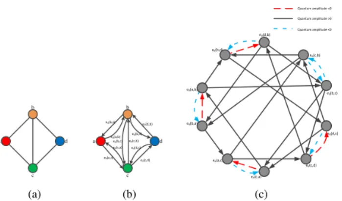
b d c a (a) b d c a ed(a,b) ed(b,a) ed(c,a) ed(a,c) ed(c,d) ed(d,c) ed(c,b) ed(b,c) ed(b,d) ed(d,b) (b) ed(a,b) ed(b,a) ed(a,c) ed(c,a) ed(c,d) ed(d,c) ed(b,c) ed(c,b) ed(d,b) ed(b,d) Quantum amplitude =0 Quantum amplitude >0 Quantum amplitude <0 (c)
Fig. 1. (a) A demo graph with 4 nodes; (b) The demo graph in (a) whose edges are all replaced by the directed edge setEd; (c) The directed line graph
GL(VL, EL). Note that discrete-time quantum walk based on the Grover diffusion matrix can be regarded as a walk on GL. The red dashed arcs, black solid arcs, and blue dash-dot arcs represent that the quantum transition amplitudes are 0, positive and negative, respectively.
Definition 1. Graph.A graph is a tuple G(V, E), where V
represents all the nodes in the graph with a set of the adjacent relationE⊆V ×V.
In this paper, we will mainly focus on connected and unattributed graphs, in which all the nodes have no attributes and all the edges have no weights and directions. Only the structural information can be used to perform the graph analysis.
Definition 2. Walk.A walk w= (v0, v1,· · ·, vk)in a graph
G(V, E) is a node sequence with vi ∈ V, and (vi, vi+1) ∈
E. The length ℓ(w) = k of a walk is the number of edges traversed in the sequence.
Definition 3. Walk set.The order-kwalk set of a graph is the set of all walks of length k which exist in a graph: W(k) =
{w|ℓ(w) =k}.
Definition 4. Subgraph(or substructure).A graphG′(V′, E′)
is a subgraph of graph G(V, E), if and only ifV′ ⊆V and
E′⊆E.
Definition 5. Graph isomorphic(or graph matching).A graph
G(V, E)is isomorphic to G′(V′, E′), if there exists at least
one bijective mapping f : V → V′ so that ∀v
1, v2 ∈
V,(v1, v2)∈E⇔(fv1, fv2)∈E ′.
B. Discrete-time quantum walk
The discrete-time quantum walk (DTQW) is the quantum counterpart of the discrete-time classical random walk [36]. In discrete-time quantum walk, the states need to specify both the current and the previous location of the walk, because of the reversibility of quantum processes. Therefore, the state space for discrete-time quantum walk is the directed edge set.
Definition 6. Directed edge setEd.In an unattributed graph
G(V, E), every edge e(u, v) ∈ E is replaced with a pair of directed edges ed(u, v) and ed(v, u). These directed edges
construct the directed edge set Ed, which can be shown as
follows.
For a demo graph shown in Fig. 1(a), the corresponding graph with directed edges is given in Fig.1(b). On the directed edge set, the directed line graph can be constructed.
Definition 7. Directed line graphGL(VL,EL).For a graph
G(V, E), its directed edge set isEd. The directed line graph
GL(VL, EL) is a dual representation of the original graph.
And the node set and edge set are defined as follows,
VL=Ed,
EL={(ed(i, m), ed(m, j))∈Ed×Ed}. (4)
Fig.1(c) shows the directed line graph of the demo graph in Fig.1(a). In the directed line graph GL(VL, EL), each
node corresponds to a unique directed edge residing on the corresponding edge in the original graph G(V, E).
In discrete-time quantum walk, if there is a directed edge from a node vL ∈ VL to a node uL ∈ VL, the transition
of the quantum walk on G(V, E) is allowed from the edge corresponding tovLto the edge corresponding touL, and vice
versa. Therefore, different with the classical random walk, the discrete-time quantum walk on a graph Gcan be regarded as a walk performed on its directed line graph GL. The state
space of the walk is the node set VL, and the transitions are
constrained by the directed edgeELin the directed line graph.
We denote the state corresponding to the quantum walker being on the directed edge ed(u, v) as |uvi. It can be
inter-preted as that a quantum particle is currently at nodevand has a previous step at node u. The general state of discrete-time quantum walk is:
|φi= X
ed(u,v)∈Ed
αuv|uvi, (5)
where the quantum amplitudeαuv is complex, i.e.,αuv∈C.
The probability that the quantum walker is at the state |uvi is given by Pr (|uvi) = αuvα∗uv, where α∗uv is the complex
conjugate ofαuv.
At each step, the evolution of the discrete-time quantum walk is governed by a transition matrix U. The entries of
U determine the transition probabilities between states, i.e., |φt+1i = U|φti. Since the evolution of the walk is linear
and conserves probability, the matrixU must be unitary, i.e.,
U−1=U†, where U† denotes the Hermitian transpose of U.
It is common to adopt the Grover diffusion matrix as the transition matrix. This matrix does not distinguish any forward nodes (i.e. those other than the current and previous nodes) and, among such diffusion matrices, it is the furthest from the identity one. The entries of the transition matrixU are shown as follows:
Uim;nj =
AimAnj(d2m −δij), if m=n
0, otherwise (6)
HereUim;njshows the quantum amplitude for the transition
ed(i, m)→ed(n, j),dmdenotes the node degree for nodem
andδij is the Kronecker delta, i.e.,δij= 1ifi=j, otherwise
δij = 0.Ais the adjacency matrix of the original graph.
Different from the random walk where the probability prop-agates, what propagates during the discrete-time quantum walk
is quantum amplitude. Given a state |imi, the Grover matrix assigns the same amplitude to all transitions|imi → |mji, and a different amplitude to the transition |imi → |mii, wherei
andj are the adjacent nodes ofm. Therefore, in the directed line graph as shown in Fig.1(c), when the particle tracks back anddm>2, the transition amplitude is negative for this step
(the blue dash-dot arc); when the particle tracks back and
dm = 2, the transition amplitude of this step is equal to 0
(the red dashed arc); otherwise, it is positive (the black solid arc). Obviously, the totter problem of random walk will be settled via the amplitude penalties for back tracks.
Furthermore, it is observed in [37] and [38] that the directed line graph possesses some special properties that are not available in the original graph. For instance, compared to the original graph, the directed line graph spans a higher dimensional feature space and thus exposes richer graph characteristics. This is because the cardinality of the node set for the directed line graph is greater than, or at least equal to, that of the original graph. This property suggests that the discrete-time quantum walk may reflect richer graph character-istics than the classical random walk and the continuous-time quantum walk, which are both the walks on the original graph.
III. R-CONVOLUTION KERNEL BASED ON FAST
DISCRETE-TIME QUANTUM WALK
In this section, a novel substructure matching method is designed based on the discrete-time quantum walk via intro-ducing the neighborhood-pair substructure. One of the issues with using the DTQW for probing graph structure is that the transition matrix U is of size 2|E| ×2|E| and so potentially quadratically bigger that the random walk equivalent. In turn this means a computation time of O(N6) in the worst case
of dense edges, which is quite impractical even for moderate-sized graphs. In order to solve this problem, a fast recursive method to calculate an alternative transition matrix is pro-posed. All these preparations lead to the newly proposed kernel FQWK.
A. Neighborhood-pair substructure matching based on discrete-time quantum walk
In this paper, the structural features based on the neighborhood-pair substructure are analyzed, which is a kind of auxiliary substructure. The formal definition is as follows.
Definition 8. k-level neighborhood-pair substructureS(abk).In a graph, for each node pairaandb, thek-level neighborhood-pair substructure Sab(k) is constructed which contains all the
k-length walks betweenaand b.
Sab(k)=nw∈W(k)|v
0=a, vk =b
o
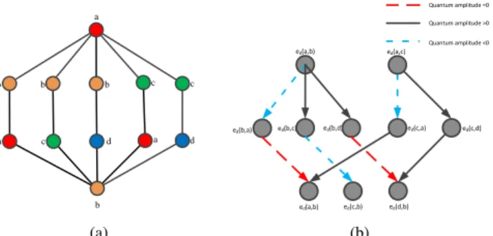
(7) Fig.2(a) illustrates that in the demo graph in Fig.1(a), there are totally 5 3-length walks from nodeato nodeb, which make up the auxiliary substructureSab(3). All the walk-based kernels can be regarded as counting over the auxiliary substructure
Sab(k). For example, there are 5 walks contributing to the RWK. The SPK and GHK compare only one walk which is the non-repeating path (acdb). Similarly, the BWK counts the single
b d c a c b d a a c b b (a) ed(a,b) ed(a,c) ed(b,a) ed(b,c) ed(b,d) ed(a,b) ed(c,b) ed(d,b) ed(c,a) ed(c,d) Quantum amplitude =0 Quantum amplitude >0 Quantum amplitude <0 (b)
Fig. 2. (a) The 5 3-length walks from nodeato nodeb; (b) The corresponding 5 2-step quantum walks on the directed line graphGL.
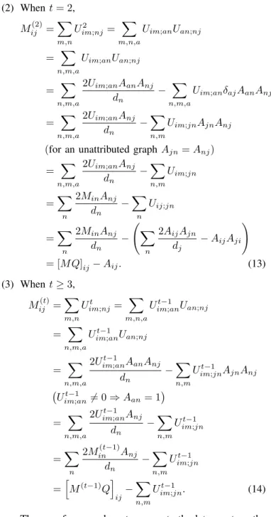
Quantum amplitude =0 Quantum amplitude >0 Quantum amplitude <0 ed(b,a) ed(a,b) ed(a,b) b a Transition Amplitude 0 ed(a,b) ed(b,c) ed(c,b) b c -2/9 ed(b,d) ed(d,b) ed(a,b) 0 a b d b ed(c,a) ed(a,b) ed(a,c) -1/3 a c ed(c,d) ed(d,b) ed(a,c) 2/3 d c 1/9
Fig. 3. Quantum transition amplitudes of the 5 3-length walks and the neighborhood-pair substructureSab(3).
non-backtracking walk(acdb). However, the BWK, GHK and SPK do not account for the edges (ab) and (bc) and the RWK treats all 5 paths identically. Therefore, the topology characteristics of this substructure cannot be well represented by the aforementioned simple features.
Our goal is to consider all these walks in Sab(k) via a superposition of the quantum amplitudes. As shown in Fig. 2(b), the 5 3-length walks correspond to the 5 2-step discrete-time quantum walks on the directed line graph given in Fig. 1(c). According to (6), the transition amplitudes of each walk can be calculated. And we use different line types to denote that the walk is positive, negative or 0. In Fig.3, we show explicitly that among all of the 5 3-length walks, there are 2 walks with quantum amplitudes 0, 2 with negative amplitudes and 1 with positive amplitude.
As we noted earlier, it is too expensive to compute the amplitude for each individual walk. Instead, we would like to compute the superposition of all the walks inSab(k), for example with Sab(2) this includes all walks of length 2 and therefore every walk which begins at a and ends at b via any single intermediate node. This can be calculated by the summation of amplitudes over all possible intermediate nodes:
Mab= N X m=1 N X n=1 Uam;nb (8)
In a similar way, Ut provides the amplitudes for allt+ 1
-length walks, and again we can compute the transition am-plitude between a and b by summing the t-step quantum
0 0 1 2 1 2 0 0 1 0 1 3 1 3 0 1 3 1 2 0 1 2 0 0 0 0 -1 3 2 3 2 3 0 0 0 0 0 0 0 0 0 1 0 0 0 2 3 -1 3 2 3 0 0 0 1 0 0 0 0 0 0 0 0 1 0 0 0 0 0 0 0 0 0 0 0 1 0 1 0 0 0 0 0 0 0 0 0 0 2 3 2 3 -1 3 0 0 Transition matrix of discrete-time quantum walk
Transition matrix of random walk -1 3 2 3 1 2 3 2 3 -1 3 0 2 3 1 0 1 1 2 3 2 3 1 -1 3
Superposition amplitude matrix of discrete-time quantum walk
Fig. 4. A demo graph and the comparisons of its three transition matrices.
amplitudes over all possible first and last steps:
Mab(t)= N X m=1 N X n=1 Ut am;nb (9)
This superposes all t-step quantum walks which start ataand end atb, i.e. all the walks inSab(t+1). This defines the transition matrixM(t).
Note that the superscripttmeans thetthpower of a matrix,
while the superscript (t) is the level index. In Fig.3, the summation of the amplitudes of these 5 walks achieves 1/9, which is just the superposition amplitude of the auxiliary substructureSab(3).
It is interesting that quantum interference exists in the quantum walk on a graph and is therefore present in our transition matrixM(t). Destructive interference will happen on
the intersection of two isomorphic substructures with opposite amplitudes [34], which is always exploited to locate the local symmetric subgraphs. On the other hand, constructive interference may occur on the crossings of different quantum walks, thereby the slight structural difference can be amplified. We choose this particular transition matrix for our graph kernel based on three factors. Firstly, it is more compact than the DTQW, since it is only of size|V|×|V|. Secondly it retains information about constructive and destructive interference since it is a superposition of individual walks. Finally, as we demonstrate in the next section, it can be computed efficiently in onlyO(t|V|3)steps in contrast to theO(t|V|6)steps of the
DTQW.
B. Fast simulation method
According to the definition, after a t-step discrete-time quantum walk, the superposition amplitude matrix M(t) is
computed as, Mij(t)= N X m=1 N X n=1 Ut im;nj 6= Mt ij. (10)
Obviously, though the size of the transition matrix M is only|V| × |V|, as shown in Fig.4,M(t)cannot be computed
via the exponential operation ofM. However, the computation complexity of the exponential operation of U is still about O |V|6
i a n j
length = t-2 length = t-1
Fig. 5. At-step quantum walk from nodeito nodej. Nodenis the previous step of nodej. Nodeais the previous step of noden.
matrix of random walk. Therefore, it is not time-acceptable to perform graph processing directly.
In Fig.4, the demo graph contains 4 nodes and 8 directed edges. The size of the transition matrix of the random walk is 4×4 because the state space of random walk is the node set. However, the size of the quantum walk transition matrix is 8×8 as the state space is the directed edge set.
Therefore, we need to find a fast method to simulate the discrete-time quantum walk and compute the matrixM(t). In
Fig.5, an arbitrary t-step discrete-time quantum walk from node i to node j is shown as an example. This walk is consisted of a (t−1)-step quantum walk from i to n and a 1-step walk fromntoj. We find a recursive method for fast computing the superposition transition matrices oft−2,t−1 andt-step discrete-time quantum walk.
Theorem 1. Assume a graph has N nodes. A is the
adjacency matrix and dn is the degree of node n. Let a
diagonal matrix D=diagd21,
2
d2,· · · ,
2
dN
and let another matrix Q = DA. The series of the superposition amplitude matrices
M(t) can be computed as,
M(t)= AQ−2D−1, t= 1 M Q−A, t= 2 M(t−1)Q−M(t−2), t≥3 (11)
Proof. (1) Whent= 1, for every item in matrixM,
Mij= X m,n Uim;nj= X m Uim;mj (Uim;nj 6= 0⇒m=n) =X m 2AimAmj dm −X m δijAimAmj = AQ−2D−1 ij (12) (2) Whent= 2, Mij(2)=X m,n Uim2 ;nj= X m,n,a Uim;anUan;nj = X n,m,a Uim;anUan;nj = X n,m,a 2Uim;anAanAnj dn − X n,m,a Uim;anδajAanAnj = X n,m,a 2Uim;anAnj dn −X n,m Uim;jnAjnAnj
(for an unattributed graph Ajn=Anj)
= X n,m,a 2Uim;anAnj dn −X n,m Uim;jn =X n 2MinAnj dn −X n Uij;jn =X n 2MinAnj dn − X n 2AijAjn dj −AijAji ! = [M Q]ij−Aij. (13) (3) Whent≥3, Mij(t)=X m,n Uimt ;nj= X m,n,a Uimt−;1anUan;nj = X n,m,a Uimt−;1anUan;nj = X n,m,a 2Uimt−;1anAanAnj dn −X n,m Uimt−;1jnAjnAnj Ut−1 im;an6= 0⇒Aan= 1 = X n,m,a 2Ut−1 im;anAnj dn −X n,m Ut−1 im;jn =X n 2Min(t−1)Anj dn −X n,m Ut−1 im;jn =hM(t−1)Qi ij− X n,m Ut−1 im;jn. (14)
Then we focus on how to compute the later part on the right-hand side of the above equation.
X n,m Ut−1 im;jn= X n,m,a Ut−2 im;ajUaj;jn = X n,m,a 2Uimt−;2ajAjn dj −X n,m Uimt−;2nj =X n 2Mij(t−2)Ajn dj −Mij(t−2) =Mij(t−2). (15)
So we get M(t)=M(t−1)Q−M(t−2). This is exactly
the formula stated inTheorem 1when t≥3.
From Theorem 1, all the operations in this recursion are no more than O(N3) for a graph withN nodes. It means that
the series matricesM(t)can be computed in cubic time of the
graph size.
C. Kernel design
1) Kernel definition for two graphs: Here we will propose a novel graph kernel based on the fast discrete-time quantum walk, named FQWK.
As a novel R-convolution kernel, the FQWK for two graphs
GA andGB is defined as follows.
KF QW K(GA, GB) =
X
t
Kt(GA, GB). (16)
After the tth step, a sub-kernel K
t(GA, GB) will be
per-formed to count all thetth-level isomorphic neighborhood-pair
substructures. The formal definition of the sub-kernel is
Kt(GA, GB) = X m,n∈GA X u,v∈GB ∆S(t) mn, Suv(t) , (17)
where∆ is a Dirac function as follows: ∆ St mn, Stuv = 1, ifMmn(t) =Muv(t), 0, otherwise. (18)
HereMmn(t) andMuv(t)are the quantum superposition
ampli-tude of the t-level neighborhood-pair substructure Smn(t) and
S(uvt), in the graph GA andGB respectively.
2) Kernel computation for a graph dataset: In the above definition, the computation of the simulation of the DTQW is the most time-consuming procedure. Therefore for a graph dataset with many graphs, this procedure needs to be per-formed only once on each graph actually, before the pairwise kernel computation.
Suppose that a graph dataset includes K graphs and each one hasN unattributed nodes.
Firstly, a T-step discrete-time quantum walk will be pro-cessed step-by-step on every graph. By using the fast simula-tion method, the superposisimula-tion matricesM(t)can be computed
according to Theorem 1. In order to reduce the amplitude comparisons, for the ith matrices M(i) of every graph G,
the histogram of all the N2 items is constructed as the ith
feature FG(i) of graph G. Therefore, for each graph, a T -dimension feature vector can be extracted. The pseudo code for the implementation of graph feature extraction algorithm is shown inAlgorithm 1.
And then, for each graph pair GA andGB in the dataset,
every feature pair FG(tA) and FG(tB) will be compared to ob-tain the number of the neighborhood-pair substructures with the same quantum superposition amplitude. For convenience of calculations, for every feature pair FG(tA) and FG(tB), an aligned and padding operation will be performed to obtain
f(t)
GA and f
(t)
GB, so that the the inner product D f(t) GA,f (t) GB E is just the frequency of the isomorphic substructure pairs. The implementation of the proposed kernel FQWK is shown in
Algorithm 2. For the input graph dataset, the algorithm of FQWK can output a kernel matrix KF QW K ∈RK×K, where
the entryKF QW K(Gi, Gj)denotes the number of isomorphic
neighborhood-pair substructures of Gi andGj.
Algorithm 1 Graph Feature Extraction Algorithm
Require: Graph G, with N nodes; di, i= 1,· · ·, N are the
node degrees;T is the fixed step of discrete-time quantum walk,T ≥3.
Ensure: FG(t): thet-step feature of G,t= 1,· · · , T.
1: function GraphF eature(G, T)
2: Get the adjacency matrixA
3: D=diag 2 d1, 2 d2,· · ·, 2 dN 4: M ←ADA−2D−1 5: FG(1) ←histogram(M) 6: M(2)←M DA−A 7: FG(2) ←histogram M(2) 8: fort= 3→T do 9: M(t)←M(t−1)DA−M(t−2) 10: FG(t)←histogram M(t) 11: end for 12: end function Algorithm 2 F QW K Algorithm
Require: Graph dataset {G1, G2,· · ·, GK}, where K
de-notes the number of graphs in the dataset; T is the fixed step of node-to-node discrete-time quantum walk, T ≥3.
Ensure: Graph kernelKF QW K ∈RK×K
1: fori= 1→K do
2: FG(t)
i ←GraphF eature(Gi, T),t= 1,· · ·, T
3: end for
4: foreach graph pair Gi andGj do
5: fort= 1→T do 6: f(t) Gi,f (t) Gj =alignment FG(ti), FG(tj) 7: Kt(Gi, Gj)← D f(t) Gi,f (t) Gj E 8: end for 9: KF QW K(Gi, Gj) =PTt=1Kt(Gi, Gj) 10: end for
Finally, we will evaluate the time complexity of calculat-ing the kernel matrix. For each graph G of the dataset, a
T-step discrete-time quantum walk needs to be performed firstly to extract the T-dimension feature vector FG. It will
cost no more than O KT N3+KT N2logN
for line 1-3 in Algorithm 2. And in line 4-9, to compute the kernel matrix, for all the graph pairs, the neighborhood-pair matching procedures are performed which cost about O K2T N2
. Overall, the total time complexity of N2QWK is about O KT N3+N2logN
+K2T N2
.
D. Discussion
1) Kernel validation: According to the Mercer’ theorem [39], a valid graph kernel must be symmetric and positive semi-definite (p.s.d.). Here we will give a brief proof of the validation of FQWK.
Theorem 2. The proposed graph kernel FQWK is valid.
Proof. The FQWK is symmetric and p.s.d, and thus, it is valid.
• Symmetric.
Based on the definition of FQWK in (16), it is obvious
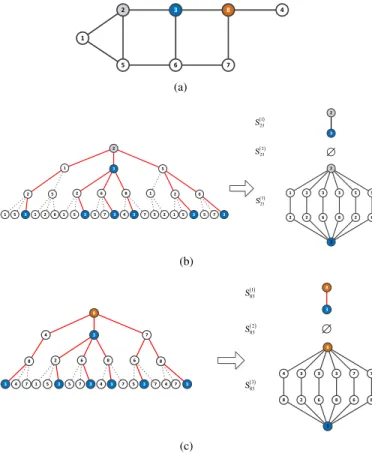
1 5 2 6 3 7 4 8 (a) 2 3 3 3 5 5 1 2 6 8 2 6 2 3 2 1 3 5 2 5 2 6 8 1 2 6 1 5 3 1 2 6 1 5 3 5 7 3 4 3 7 5 2 1 5 3 5 7 3 1 23 S 3 23 S 2 3 2 23 S (b) 8 3 3 3 7 7 4 2 6 8 6 8 8 3 8 4 3 7 8 2 6 8 6 8 3 4 7 1 5 3 5 7 3 4 3 7 5 3 7 4 7 3 1 83 S 8 3 2 83 S 3 83 S (c)
Fig. 6. (a) An example graph with node 8; (b) The 3-level neighborhood of nodev2and the substructuresS23(1),S
(2)
23 andS
(3)
23; (c) The neighborhood of
v8and the substructuresS83(1),S (2)
83 andS
(3)
83.
• p.s.d.
In the definition of FQWK, after the tth step of
quan-tum walk, a matching sub-kernel Kt(GA, GB) will
be performed to count all the tth-level isomorphic
neighborhood-pair substructures. It is known that the summation kernel of some p.s.d. ones is still p.s.d. Be-cause Dirac function is p.s.d, the sub-kernelKt(GA, GB)
is p.s.d. Therefore, FQWK is p.s.d.
2) Theoretical analysis of FQWK: From the above defini-tion, FQWK seems an instance of walk-based graph kernels. It is close to RWK and BWK because we only use discrete-time quantum walk to replace classical random walk and backtrack-less walk. Therefore, the computation procedure of FQWK is comparatively simple compared with other R-convolution kernels.
Besides, compared with RWK and BWK, the proposed FQWK can represent more powerful structural characteristics. The reason is analyzed using the following example. Fig.6(a) shows an example graph with 8 nodes. Focus on two node pairs: node v2 to node v3 and node v8 to node v3. The
neighborhood of node v2 and node v8 as well as the 1 to 3
level neighborhood-pair substructures are shown in Fig.6(b) and Fig.6(c), respectively. Obviously, both S23(1) and S83(1)
have only 1 walk (path). S(2)23 and S (2)
83 are both empty.
Meanwhile there are 6 3-length walks included in S23(3) and
(a) (b)
Fig. 7. Two example graphs with node 8.
S83(3), and only 1 path (or backtrackless walk) exists in each
of them, namely v2v5v6v3 andv8v7v6v3, respectively. Based
on the counting of walks or paths, the neighborhood-pair substructures are isomorphic when using the RWK and other walk-based kernels. Therefore, node v2 and node v8 can be
matched. However, it is obvious that the nodev2 and nodev8
should not be matched as the adjacent nodev1andv4 cannot
be matched. Therefore, classification error will be caused by using the RWK and BWK if such kind of structures exist. If the proposed FQWK is used, the superposition amplitude of the substructure Sv(3)2v3 is −1/9, which is different with the substructureSv(3)8v3 with amplitude 1, so the two substructures don’t match. Therefore, the proposed FQWK outperforms the existing walk-based kernels as more powerful features can be represented by the auxiliary substructure S(abk). The false-positive substructure matching will be reduced and the classification performance can be improved by the FQWK.
Actually, FQWK is a member of the subgraph-based kernel family as the core procedure is the neighborhood-pair sub-structure matching based on the comparison of the quantum superposition amplitudes over the sets Sab(k), rather than the counting of individual walks. Compared with the existing subgraph-based kernels, the FQWK is better because the relative position between the substructures is considered. For the graph in Fig.6(a) and two graphs in Fig.7, 1 triangle and 2 squares are included in all the three example graphs, but the relative position among these 3 graphlets are different. Therefore, the three graphs should not be matched. In the computation of the traditional subgraph-based kernels, the relative position between the adjacent substructures are usually ignored in the traditional kernel computation, which will lead to the error matching of the three graphs. In FQWK, the auxiliary substructureSab(k)can be regarded as the intersection between thek-level neighborhood of nodea and nodeb, and quantum superposition amplitude of every neighborhood-pair substructure S(abk) will be affected by two kinds of quantum interference:
• The inter interference among all the quantum walks
which are included in the neighborhood-pair substruc-ture. In Fig.6(b) and Fig.6(c), the red solid lines denote these included quantum walks. The quantum interference among them will affect the superposition amplitude of the substructureSab(k).
• The intra interference from the adjacent
neighborhood-pair substructures. In Fig.6(b) and Fig.6(c), the black dashed lines denote the quantum walks excluded inSab(k). However, via quantum interference, the superposition
amplitude of one substructure will also be affected by its adjacent ones.
Therefore, compared with other subgraph-based methods, FQWK can extract more powerful substructure features by catching more extra information of the location relationships of local substructures.
Previous work on quantum walks [28], [32], [34] has shown that quantum walks are sensitive to structures which random walks are not. We demonstrate empirically in Section IV that our transition matrix retains these properties and produces excellent performance on standard datasets.
IV. EXPERIMENTS
In this section, the newly proposed kernel FQWK is evaluat-ed on classification problems for unattributevaluat-ed graphs. Here we perform a fast discrete-time quantum walk in the computation of FQWK. In the test, we choose the user-defined fixed step
T as 10. The discussion of the choice of parameterT is given in Section IV-B3. And we also compare FQWK with several other popular graph classification methods as follows.
• Random walk kernel (RWK). The version of [40] is used
to test.
• Weisfeiler-Lehman kernel (WLK) [10]. For the sake of
fairness, the highest dimension of the Weisfeiler-Lehman isomorphism is set to be 10.
• GraphHopper kernel (GHK) [17]. The Dirac kernel is used to be the base node kernel.
• All graphlet kernel (AGK) [22]. The graphlet size is
chosen to be 4.
• Aligned subtree kernel (ASK) [11]. The density matrix
of continuous-time quantum walk is used to enhance the node attributes. And the entropic representation layer is also set to be 10. For WLK, GHK and ASK, we use node degree as the original node attribute for unattributed graphs.
• Quantum Jensen-Shannon kernel (QJSK) [32]. The
den-sity matrix of 10-step discrete-time quantum walk is used for the computation of Von Neumann entropy .
• Edge-based matching kernel based on discrete-time
quan-tum walk (DQMK) [35]. A 10-step discrete-time quanquan-tum walk is used to perform edge matching and the highest layer of the depth-based representation is set to be 10.
• PATCHY-SAN convolutional neural
net-work(PSCN) [41]. Similar with the behavior of CNNs on images, PSCN first extracts fixed-sized local patches from nodes and neighborhoods as the receptive fields for convolution filters and then use the graph canonization tool NAUTY to apply CNNs on these patches. Here we set the receptive field size as 10.
• Deep graph convolutional neural network (DGCNN)
[42]. DGCNN inherits the PSCN idea of imposing an order for graph nodes, but integrates this step into the network structure, namely the SortPooling layer. We set the sortpooling parameter as 0.6 and learning rate as 0.0001. Both PSCN and DGCNN are trained with epochs 150 and batch size 25.
TABLE I
THE DETAILED INFORMATION OF THE REAL-WORLD DATASETS
Dataset #Set #Class Avg.#Node Avg.#Edge
AIDS 2000 2 15.69 16.20 COX2 467 2 41.22 43.45 DHFR 756 2 42.43 44.54 ENZYMES 600 6 32.63 62.14 MUTAG 188 2 17.93 19.79 NCI1 4110 2 29.87 32.30 PTC MM 336 2 13.97 14.32 TABLE II
THREE NON-ISOMORPHIC GRAPH DATASETS. INCOSGRAPH,EVERY
COSPECTRAL GRAPH PAIR IS USED AS A TEST. INREGGRAPH AND
SRGRAPH,PAIR-WISE COMPARISONS OF THE GRAPHS IN EACH CLASS
ARE EVALUATED
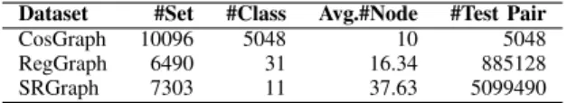
Dataset #Set #Class Avg.#Node #Test Pair
CosGraph 10096 5048 10 5048
RegGraph 6490 31 16.34 885128
SRGraph 7303 11 37.63 5099490
All the experiments were tested in Matlab R2016b on an Intel Xeon Core E5-1620 CPU with 8 GB memory. All the runtime consumption tests were executed with a single thread.
A. Datasets
Both real-world and synthetic datasets are used to evaluate the graph kernels.
The real-world datasets. To evaluate the classification accuracy, 7 chemical datasets with ground truth labels are collected [43]. All the chemical molecules are converted into unattributed graphs by representing atoms as nodes and the covalent bonds as edges.
AIDS consists of graphs representing molecular com-pounds from the AIDS Antiviral Screen Database of Ac-tive Compounds. There are 2,000 elements totally (1,600 inactive elements and 400 active elements), which represen-t molecules wirepresen-th acrepresen-tivirepresen-ty againsrepresen-t HIV or norepresen-t. COX2 has 467 cyclooxygenase-2 inhibitors has been assembled in this dataset. DHFR is consisted of 756 inhibitors of dihydrofolate reductase for the inhibition of the enzymatic reduction that converts dihydrofolate to tetrahydrofolate. ENZYME collects 600 graphs representing tertiary protein structures, each la-beled with one of the 6 EC top-level classes. MUTAG includes 188 graphs representing mutagenetic compounds, labeled ac-cording to their mutagenic effects. NCI1 is a set of 4110 graphs representing a subset of chemical compounds screened for activity against non-small cell lung cancer cell lines. The Predictive Toxicology Challenge (PTC) dataset records the carcinogenicity of several hundred chemical compounds. These graphs are very small and sparse, with 20-30 nodes, and 25-40 edges. We select the graphs of male mice (PTC MM) for evaluation. There are 336 test graphs in the MM class.
Table I shows the statistical information of these chemical datasets.
The synthetic datasets. In order to further evaluate the distinguishing ability of the kernels, some special datasets are chosen [44] as shown in Table II. CosGraph includes
TABLE III
THE AVERAGE ACCURACY(IN%±STANDARD ERROR)ON GRAPH CLASSIFICATION BENCHMARK DATASETS
Methods
Datasets
AIDS COX2 DHFR ENZYMES MUTAG NCI1 PTC MM
RWK 80.00±.28 78.20±.61 60.96±.56 14.20±.42 80.56±.72 53.16±.30 61.59±.86 WLK 98.89±.07 79.38±.57 82.43±.45 37.69±.62 83.22±.89 81.87±.20 61.72±.81 GHK 99.33±.58 78.65±.89 79.77±.75 37.34±.58 85.40±.85 68.02±.36 61.45±.59 AGK 99.07±.07 78.20±.61 60.96±.56 28.88±.61 82.01±.90 62.54±.25 63.65±.82 PSCN 99.53±.03 77.66±.14 60.00±.27 15.50±.09 83.16±1.1 56.91±.09 59.41±.34 DGCNN 98.50±.03 78.26±.46 66.67±.26 40.12±.11 77.78±.51 69.34±.44 54.55±.76 ASK 96.74±.12 78.17±.61 74.15±.48 30.26±.60 84.96±.84 64.52±.24 61.15±.81 QJSK 79.57±.28 78.73±.61 78.41±.47 34.61±.62 83.62±.68 67.20±.22 60.58±.85 DQMK 79.99±.67 78.15±.64 76.77±.96 28.91±.71 76.42±.88 65.18±.33 61.09±.73 FQWK 99.53±.06 80.87±.57 82.92±.41 41.55±.61 84.27±.83 80.39±.19 63.77±.78 TABLE IV
COMPUTATION TIME OF THE GRAPH CLASSIFICATION METHODS(FOR GRAPH KERNELS,WE FOCUS ON THE COMPUTATION TIME OF KERNEL MATRIX.
FOR GRAPH NEURAL NETWORKS,THE TRAIN TIME OF THE NETWORK MODEL IS LISTED. THE LAST FOUR KERNELS ARE DESIGNED BASED ON THE
QUANTUM WALK)
Methods
Datasets
AIDS COX2 DHFR ENZYMES MUTAG NCI1 PTC MM
RWK 37′7′′ 6′4′′ 8′16′′ 4′20′′ 15′′ 197′13′′ 50′′ WLK 26′′ 7′′ 23′′ 15′′ 2′′ 1′57′′ 2′′ GHK 24′41′′ 2′42′′ 6′23′′ 4′49′′ 14′′ 164′11′′ 35′′ AGK 26′′ 15′′ 23′′ 32′′ 3′′ 1′34′′ 4′′ PSCN 1′48′′ 47′′ 1′21′′ 1′7′′ 14′′ 5′57′′ 20′′ DGCNN 4′5′′ 1′30′′ 2′32′′ 1′54′′ 23′′ 11′43′′ 44′′ ASK 92′25′′ 28′50′′ 61′16′′ 25′5′′ 1′25′′ 773′58′′ 2′51′′ QJSK 141′58′′ 21′18′′ 58′2′′ 23′50′′ 1′3′′ 611′10′′ 2′32′′ DQMK 97′44′′ 28′51′′ 76′37′′ 88′56′′ 1′26′′ 1203′9′′ 2′53′′ FQWK 38′52′′ 8′47′′ 13′57′′ 5′15′′ 27′′ 269′50′′ 58′′
5048 pairs of 10-node graphs. Each pair of graphs has the same graph spectrum, which is called a cospectral graph pair. RegGraph and SRGraph consist of 31 classes of regular graphs and 11 classes of strong regular graphs respectively. Within each class, every graph is regular or strong regular but not isomorphic with others.
B. Results
1) Test result for graph classification: Graph classification is an important application which is quite related to the measurement of the graph similarity. Here we investigate the performance of the novel graph kernel for the datasets in Table I.
For each dataset, 10-fold cross-validation tests are per-formed using all the mentioned methods. For graph kernels, the classification accuracy is accomplished via using the C-Support Vector Machine (C-SVM) with the optimal parameters [45]. The average accuracy (± standard error) and runtime results are reported in Table III and Table IV.
Table III reports the average classification accuracy and the relative standard error of each method and dataset. For the datasets AIDS, COX2, DHFR, ENZYMES and PTC MM, the new kernel FQWK achieves the highest accuracy, which yields a remarkable improvement compared with the other state-of-the-art kernels and graph neural networks. Only for MUTAG and NCI1, GHK and WLK show a slight better performance than FQWK respectively. Although the classification for u-nattributed graphs is quite difficult, FQWK turns out to be
the best competitor in terms of accuracy on most of these benchmark datasets.
The reasons for the effectiveness are threefold.
• a) Owing to the powerful discrimination of quantum
in-terference, FQWK can establish the substructure location relationship which is deficient in the traditional methods RWK, WLK, GHK, AGK, PSCN and DGCNN.
• b) Compared with the information theoretic kernel QJSK
which computes the graph similarity via the global structural information, FQWK can reflect richer local convolutional characteristics of graphs via performing step-by-step evolution of discrete-time quantum walk.
• c) The quantum walk kernels ASK and DQMK perform
the edge matching and subtree matching to compute graph similarity. While FQWK can capture finer-grained features of graphs via matching the neighborhood-pair substructures.
Table IV shows the runtime comparison of these classifi-cation methods for each dataset. FQWK achieves a moder-ate performance. However, compared with ASK, QJSK and DQMK, FQWK is the fastest one among all the kernels based on quantum walk. Via the fast recursive method, the runtime of FQWK is close to that of RWK.
2) Test result for distinguishing ability: Some similar and non-isomorphic graphs are usually difficult to distinguish via inexact graph comparison methods. Therefore, a graph kernel cannot be applied to some kinds of graphs. Here the distinguishing ability for similar graphs is used to compare the applicability of these graph kernels. We utilize the failure rate
TABLE V
THE FAILURE RATES(%)FOR DISTINGUISHING THE NON-ISOMORPHIC
GRAPHS(-DENOTES THE TEST CANNOT BE FINISHED BY THE KERNEL IN
10DAYS). HERE ONLY GRAPH KERNELS ARE CONSIDERED TO BE TESTED.
Kernel Name CosGraph RegGraph SRGraph
RWK 100 100 100 WLK 1.66 100 100 GHK 18.82 0.12 100 AGK 5.96 4.87 3.82 ASK 33.16 1.14 95.96 QJSK 33.16 1.14 13.60 DQMK 0 0.11 -FQWK 0 0.02 0.0016
as the applicability measurement for the graph kernels. Table V shows the failure rates of these graph kernels for distinguishing the similar graph pairs collected in Table II, including the cospectral graphs, regular graphs and strong regular graphs.
RWK is the worst kernel, which cannot be used to dis-tinguish these similar graphs. WLK can only locate the dif-ference of the cospectral graphs, but fails for regular graphs. Generally, compared with the traditional kernels, the quantum walk kernels achieve better distinguishing ability because the slight topological difference will be amplified by quantum interference. In particular, FQWK has the lowest failure rates for all the three kinds of non-isomorphic graphs, and thus out-performs the other kernels. The powerful ability of FQWK for distinguishing non-isomorphic graphs, even including strong regular graphs, comes from the fact that both the inter and intra quantum interference of the neighborhood-pair substructures is included.
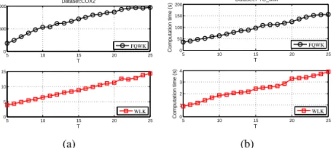
3) Test result about the parameter T: In the proposed algorithm, the maximum walk step T should be user-defined. This parameter is also used in QJSK, ASK and some other kernels to restrict the walk steps. In essence, due to the fact that the amplitude propagation occurs in the neighborhood of nodes, the maximum walk step T actually limits the order of the neighborhood-pair substructures that is explored in the algorithm. In the former tests, we set T = 10.
In this part, the influence of T is under consideration. Our proposed kernel FQWK and WLK, are tested for example using different T for the datasets COX2 and PTC MM. We change T from 5 to 25. The accuracy and computation time results are shown in Fig. 8 and Fig. 9, respectively. We find out that the accuracy keeps almost unchanged. However, the computation time has a nearly linear growth with the increase ofT. The reason is that much of the structural information has already been contained in the low order neighborhood of the node, which is quite discriminative for the graph classification based on the local structure matching. With the increasing of T, there are barely isomorphic and large substructures between two graphs so that the classification accuracy nearly maintains. Therefore, it is reasonable that we choose the same parameter T for all graph kernels which extract features via node neighborhoods.
V. CONCLUSION
In this paper, a novel R-convolution graph kernel FQWK is proposed based on the fast discrete-time quantum walk. Via the
4 6 8 10 12 14 16 18 20 22 24 26 70 75 80 85 T
Classification accuracy (%) with standard error
Dataset:COX2 FQWK WLK (a) 4 6 8 10 12 14 16 18 20 22 24 26 55 60 65 70 T
Classification accuracy (%) with standard error
Dataset:PTC_MM
FQWK WLK
(b)
Fig. 8. (a) The classification accuracy (%) and standard error of using FQWK and WLK for the dataset COX2 with different T; (b) The classification accuracy (%) and standard error of using FQWK and WLK for the dataset PTC MM with differentT. 5 10 15 20 25 0 500 1000 T Computation time (s) Dataset:COX2 FQWK 5 10 15 20 25 0 5 10 15 T Computation time (s) WLK (a) 5 10 15 20 25 0 50 100 150 200 T Computation time (s) Dataset:PTC_MM FQWK 5 10 15 20 25 0 1 2 3 4 T Computation time (s) WLK (b)
Fig. 9. (a) The computation time (s) of using FQWK and WLK for the dataset COX2 with differentT; (b) The computation time(s) of using FQWK and WLK for the dataset PTC MM with differentT.
powerful quantum interference of the discrete-time quantum walk, more reliable location correspondences between the neighborhood-pair substructures are located so that FQWK can extract finer-grained structural features, which the traditional R-convolution kernels are deficient to. Extensive experiments demonstrate the classification accuracy of FQWK outperforms that of the state-of-the-art graph kernels and the distinguishing ability for non-isomorphic graphs is significantly improved.
In addition, a novel and fast simulation method is pro-posed for computing the transition matrices of the discrete-time quantum walk, so that FQWK can achieve the highest computation speed among all the existing kernels based on the quantum walk.
ACKNOWLEDGMENT
This work is funded by Natural Science Foundation of Hunan Province, grant number 2019JJ40340, and National Natural Science Foundation of China, grant number 61701502. The authors appreciate the kind comments and professional criticisms of the anonymous reviewers. They have greatly enhanced the overall quality of the manuscript and opened numerous perspectives geared toward improving the work.
REFERENCES
[1] V. T. Ta, O. L´ezoray, A. Elmoataz, and S. Sch¨upp, “Graph-based tools for microscopic cellular image segmentation,”Pattern Recognition, vol. 42, no. 6, pp. 1113–1125, 2009.
[2] J. W. Raymond and P. Willett, “Maximum common subgraph isomor-phism algorithms for the matching of chemical structures,”J Comput Aided Mol Des, vol. 16, no. 7, pp. 521–533, 2002.
[3] W. Fan, “Graph pattern matching revised for social network analysis,” inInternational Conference on Database Theory, 2012.
[4] A. C. N. Ngomo and F. Schumacher, “BorderFlow: A local graph clustering algorithm for natural language processing,” inInternational Conference on Computational Linguistics and Intelligent Text Process-ing, 2009.
[5] P. Mah´e and J. P. Vert, “Graph kernels based on tree patterns for molecules,”Machine Learning, vol. 75, no. 1, pp. 3–35, 2009. [6] N. M. Kriege, M. Neumann, C. Morris, K. Kersting, and P. Mutzel, “A
unifying view of explicit and implicit feature maps for structured data: Systematic studies of graph kernels,”CoRR, vol. abs/1703.00676, 2017. [7] H. Bunke, “On a relation between graph edit distance and maximum common subgraph.”Pattern Recognition Letters, vol. 18, no. 9, pp. 689– 694, 1997.
[8] A. Banerjee, S. Merugu, I. S. Dhillon, J. Ghosh, and J. Lafferty, “Clustering with Bregman divergences,”Journal of Machine Learning Research, vol. 6, no. 4, pp. 1705–1749, 2005.
[9] T. G¨artner, P. Flach, and S. Wrobel, “On graph kernels: Hardness results and efficient alternatives,” in Learning theory and kernel machines. Springer, 2003, pp. 129–143.
[10] N. Shervashidze, P. Schweitzer, E. J. V. Leeuwen, K. Mehlhorn, and K. M. Borgwardt, “Weisfeiler-Lehman graph kernels,”Journal of Ma-chine Learning Research, vol. 12, no. 9, pp. 2539–2561, 2011. [11] L. Bai, L. Rossi, and E. Hancock, “An aligned subtree kernel for
weighted graphs,” in International Conference on Machine Learning, 2015, pp. 30–39.
[12] F. Aziz, R. C. Wilson, and E. R. Hancock, “Backtrackless walks on a graph,”IEEE transactions on neural networks and learning systems, vol. 24, no. 6, pp. 977–989, 2013.
[13] Y. Aharonov, L. Davidovich, and N. Zagury, “Quantum random walks,”
Physical Review A, vol. 48, no. 2, p. 1687, 1993.
[14] D. Haussler, “Convolution kernels on discrete structures,” Technical report, Department of Computer Science, University of California, Tech. Rep., 1999.
[15] L. Bai, “Information theoretic graph kernels,” Ph.D. dissertation, Uni-versity of York, 2014.
[16] K. M. Borgwardt and H. P. Kriegel, “Shortest-path kernels on graphs,” inInternational Conference on Data Mining, 2005, p. 8.
[17] A. Feragen, N. Kasenburg, J. Petersen, M. de Bruijne, and K. Borgwardt, “Scalable kernels for graphs with continuous attributes,” in Annual Conference on Neural Information Processing Systems, 2013, pp. 216– 224.
[18] Z. Zhang, M. Wang, Y. Xiang, Y. Huang, and A. Nehorai, “RetGK: Graph kernels based on return probabilities of random walks,” inAnnual Conference on Neural Information Processing Systems, 2018. [19] R. Kondor and H. Pan, “The multiscale Laplacian graph kernel,” in
Annual Conference on Neural Information Processing Systems, 2016, pp. 2990–2998.
[20] L. Bai, Z. Zhang, C. Wang, X. Bai, and E. R. Hancock, “A graph kernel based on the Jensen-Shannon representation alignment,” inInternational Joint Conference on Artificial Intelligence, 2015.
[21] G. Nikolentzos, P. Meladianos, S. Limnios, and M. Vazirgiannis, “A degeneracy framework for graph similarity,” in International Joint Conference on Artificial Intelligence, 2018.
[22] N. Shervashidze, S. V. N. Vishwanathan, T. Petri, K. Mehlhorn, and K. Borgwardt, “Efficient graphlet kernels for large graph comparison,” inArtificial Intelligence and Statistics, 2009, pp. 488–495.
[23] P. Yanardag and S. V. N. Vishwanathan, “Deep graph kernels,” in
Proceedings of the 21th ACM SIGKDD International Conference on Knowledge Discovery and Data Mining, 2015, pp. 1365–1374. [24] N. Kriege and P. Mutzel, “Subgraph matching kernels for attributed
graphs,” inInternational Conference on Machine Learning, 2012, pp. 291–298.
[25] P. Wang, J. Zhao, X. Zhang, Z. Li, J. Cheng, J. C. S. Lui, D. Towsley, J. Tao, and X. Guan, “MOSS-5: A fast method of approximating counts of 5-node graphlets in large graphs,”IEEE Transactions on Knowledge and Data Engineering, vol. 30, no. 1, pp. 73–86, 2018.
[26] N. M. Kriege, P. L. Giscard, and R. C. Wilson, “On valid optimal assignment kernels and applications to graph classification,” inAnnual Conference on Neural Information Processing Systems, 2016. [27] F. Orsini, P. Frasconi, and L. De Raedt, “Graph invariant kernels,” in
Proceedings of the AAAI Conference on Artificial Intelligence (AAAI), 2015, pp. 678–689.
[28] G. Minello, L. Rossi, and A. Torsello, “Can a quantum walk tell which is which? A study of quantum walk-based graph similarity,”Entropy, vol. 21, no. 3, 2019.
[29] L. Bai, E. R. Hancock, A. Torsello, and L. Rossi, “A quantum Jensen-Shannon graph kernel using the continuous-time quantum walk,” in
International Workshop on Graph-Based Representations in Pattern Recognition, 2013, pp. 121–131.
[30] L. Rossi, A. Torsello, and E. R. Hancock, “A continuous-time quantum walk kernel for unattributed graphs,” in International Workshop on Graph-Based Representations in Pattern Recognition, 2013, pp. 101– 110.
[31] L. Rossi, A. Torsello, and E. R. Hancock, “Measuring graph similar-ity through continuous-time quantum walks and the quantum Jensen-Shannon divergence,”Phys Rev E Stat Nonlin Soft Matter Phys, vol. 91, no. 2, p. 022815, 2015.
[32] L. Bai, L. Rossi, L. Cui, Z. Zhang, P. Ren, X. Bai, and E. Hancock, “Quantum kernels for unattributed graphs using discrete-time quantum walks,”Pattern Recognition Letters, vol. 87, pp. 96–103, 2017. [33] L. Bai, L. Rossi, H. Bunke, and E. R. Hancock, “Attributed graph kernels
using the Jensen-Tsallis q-differences,” inJoint European Conference on Machine Learning and Knowledge Discovery in Databases. Springer, 2014, pp. 99–114.
[34] D. Emms, R. C. Wilson, and E. R. Hancock, “Graph matching using the interference of continuous-time quantum walks,” Pattern Recognition, vol. 42, no. 5, pp. 985–1002, 2009.
[35] L. Bai, Z. Zhang, P. Ren, L. Rossi, and E. R. Hancock, “An edge-based matching kernel through discrete-time quantum walks,” inInternational Conference on Image Analysis and Processing. Springer, 2015, pp. 27–38.
[36] D. Emms, S. Severini, R. C. Wilson, and E. R. Hancock, “Coined quantum walks lift the cospectrality of graphs and trees,” Pattern Recognition, vol. 42, no. 9, pp. 1988–2002, 2009.
[37] L. Bai, P. Ren, and E. R. Hancock, “A hypergraph kernel from iso-morphism tests,” in International Conference on Pattern Recognition, 2014.
[38] R. Peng, T. Aleksi´c, D. Emms, R. C. Wilson, and E. R. Hancock, “Quantum walks, Ihara zeta functions and cospectrality in regular graphs,”Quantum Information Processing, vol. 10, no. 3, pp. 405–417, 2011.
[39] J. C. Ferreira and V. A. Menegatto, “Eigenvalues of integral operators defined by smooth positive definite kernels,”Archiv Der Mathematik, vol. 64, no. 1, pp. 61–81, 2009.
[40] S. V. N. Vishwanathan, K. M. Borgwardt, and N. N. Schraudolph, “Fast computation of graph kernels,” inAdvances in Neural Information Processing Systems 19, 2007.
[41] M. Niepert, M. Ahmed, and K. Kutzkov, “Learning convolutional neural networks for graphs,” inICML, 2016, pp. 2014–2023.
[42] M. Zhang, Z. Cui, M. Neumann, and Y. Chen, “An end-to-end deep learning architecture for graph classification,” inAAAI, 2018, pp. 4438– 4445.
[43] K. Kersting, N. M. Kriege, C. Morris, P. Mutzel, and M. Neumann, “Benchmark data sets for graph kernels,” 2016. [Online]. Available: http://graphkernels.cs.tu-dortmund.de
[44] Y. Zhang, L. Wang, and L. Wang, “A comprehensive evaluation of graph kernels for unattributed graphs,”Entropy, vol. 20, no. 12, p. 984, 2018. [45] C.-C. Chang and C.-J. Lin, “LIBSVM: a library for support vector machines,” ACM transactions on intelligent systems and technology, vol. 2, no. 3, p. 27, 2011.
Yi Zhang was born in Nanyang, China, in 1987. He received the B.Eng. and the Ph.D. degree in Computer Science from National University of De-fense Technology in 2009 and 2014, respectively. His research interests include quantum mechanics, machine learning and graph classification.
Lulu Wangreceived the B.Eng. and the Ph.D. de-grees in Information and Communication Engineer-ing from National University of Defense Technolo-gy, Changsha, China, in 2009 and 2015, respectively. She is currently an Assistant Professor with Artificial Intelligence Research Center, National Innovation Institute of Defense Technology, Beijing, China. Her research interests include cognitive radar, radar waveform optimization and machine learning.
Richard Wilsonreceived the B.A. degree in physics from the University of Oxford, Oxford, U.K. in 1992, and the D.Phil. degree from the University of York, York, U.K. in 1996. He is currently a Professor with the Department of Computer Science, University of York. He has authored more than 200 papers in journals, edited books, and refereed conferences. His research interests include structural pattern recognition, graph methods for computer vision and novel imaging systems. He is a fellow of the IAPR and a senior member of IEEE.
Kai Liureceived the B.Eng. degree in Computer Science from National University of Defense Tech-nology in 2016. He is currently a doctoral student in College of Computer Science, National University of Defense Technology, Changsha, China. His research interests are in the areas of quantum computation and data mining.