9.4.1 Classical Nusselt Evaporation

1.

The vapor is quiescent.

2.

Inertia in the liquid film is negligible.

3.

Heat transfer through the liquid film is by conduction

only, i.e., convective terms in the energy equation are

negligible.

4.

The properties are constant.

5.

The process occurs at steady state.

6.

A no-slip condition exists at the wall.

9.4 Falling Film Evaporation on a Heated Wall

 Assuming negligible inertia and constant fluid properties the

momentum balance is

(9.98)

 The velocity profile

(9.99)

 _{Mass flow rate per unit width}

(9.100)

 _{Film thickness}

(9.101)

 _{Considering eq. (9.101) the heat transfer coefficient becomes}

(9.102)

(

)

2 2 v

d u

g

dy

µ

l

= −

ρ

−

ρ

l l

(

)









−

−

=

2

2

y

y

g

u

v

δ

µ

ρ

ρ

  

∫

=

Γ

δ

ρ

0 

udy

(

)

3 1

3













−

Γ

=

g

v

ρ

ρ

ρ

µ

δ

  

(

)

13









−

=

k

ρ



ρ



ρ

g

h

v

 The overall energy balance across the liquid film

(9.103)

 Combining eqs. (9.102)-(9.103), one obtains

(9.104)

 _{Integrating from the inlet to some arbitrary length L}

(9.105)

 _{A relation for Γ is obtained from the inlet mass flow rate and the wall}

and vapor temperatures

(9.106)

 _{Mass flow rate width is related to Reynolds number}

(9.107)

(

)

v w v

d

h

h T

T

dx

Γ = −

−

l

(

)

1 3

(

)

1 3 3 v w v v g k d T T dx h ρ ρ ρ µ  −  Γ Γ = − _{ } −   l l l l l

(

)

1 3

(

)

1 3 0 3 L o L _v w v v g k d T T dx h ρ ρ ρ µ Γ Γ  −  Γ Γ = − _{ } −  

∫

∫

_l l l l l

(

)

1 3

(

)

4 3 4 3 4 3 3 v L o w v v g k T T L h ρ ρ ρ µ  −  Γ = Γ − _{ } −   l l l l l

Γ

=

4

Re

 The heat transfer coefficient from eq. (9.102) can be expressed in

terms of Reynolds number

(9.108)

 _{The energy flux over the entire length is balanced with the mass flux}

from the interface

(9.109)

 _{Eq. (9.103) can be written in terms of the Reynolds number}

(9.110)

 _{Integrating eq. (9.110) in the interval of (0,L)}

(

)

1 3 _{1 3} 2 1/ 3 1 3

4

1

1.10 Re

3

Re

v

h

k

g

µ

ρ ρ

ρ

−





 

=

=



−



 

 









l l l l

(

)

(

)

(

(

)

)

_ 0

Re

0

Re

4

v L v L w v w v

h

h

h

L T

T

L T

T

µ

Γ − Γ

−

=

=

−

−

l l l

(

)

4

Re

_{w v} v

T

T

d

dx

h

µ

h

−

= −

l l

(

)

4

Re

T

T L

d

−



Combining eqs. (9.109) and (9.111), the average

heat transfer coefficient is

(9.112)



Substituting eq. (9.108) into eq. (9.112) the

average heat transfer coefficient in terms of

Reynolds number is

(9.113)



Rewriting the relation for Γ in terms of Reynolds

number

(9.114)

(

)

0 _ 0 Re Re Re Re 1 Re L L h d h − = −

∫

(

)

(

(

4 3 4

)

3

)

3 4 3 1 2 _

Re

Re

Re

Re

3

4

L o L o v

g

k

h

−

−













=













−

ρ

ρ

ρ

µ

   

(

)

(

)

1 3 4 3 4 3 4 3 4 3

4

Re

Re

4

3

3

w v v L o

k T

T L

g

h

ρ ρ

ρ

µ

µ

−



−



 

=

−

 





 





l l l



Example 9.5

A liquid film flows downward and evaporates on a vertical

plate subjected to a constant heat flux. Determine the

average heat transfer coefficient.



Solution

:

The physical model of the problem under consideration is similar to that shown in Fig. 9.11 except that the thermal boundary condition is

changed. The local heat transfer coefficient for falling film evaporation can still be calculated by eq. (9.102) or (9.108),

because no assumption about boundary conditions were used to obtain them.

For the case of constant heat flux, the energy balance accounts for the heat addition required for evaporation, i.e.,

(9.115) Since is not a function of x, eq. (9.115) can be integrated in the

interval of (0, L) to yield (9.116) v w d h q dx Γ _{= − ′′} l w

q

′′

0 w q L h ′′ Γ = Γ −

 Equation (9.116) can be rewritten in terms of Reynolds number as

(9.117) which can be used to obtain the Reynolds number at x=L. The average

heat transfer coefficient can be obtained by

(9.118) which is similar to eq. (9.109) except that the wall temperature is the

average value along the wall (0<x<L), i.e.,

(9.119) 0 4 Re Re w L v q L h µ ′′ = − l l

(

)

(

)

(

(

)

)

_ 0 Re0 Re 4 v L v L w v w v h h h L T T L T T µ Γ − Γ − = = − − l l l 0 L w w

T

=

∫

T dx

 For the case with constant heat flux, the energy balance across the

liquid film in terms of Reynolds number can still be represented by eq. (9.110). Integrating eq. (9.110) in the interval of (0, L) and

considering the fact that T_w is not a constant, one obtains

(9.120)

 _{Combining eqs. (9.118) and (9.120) to eliminate yields the same}

equation as eq. (9.112), which eventually leads to eq. (9.113). Therefore, eq. (9.113) is also valid for the case with constant heat flux heating, while the Reynolds number at x = L must be calculated by eq. (9.117).

(

)

0 Re Re 4 Re L w v x v T T L d h µ h − = −

∫

_{l l}



The energy equation for a two-dimensional situation

using the vertical wall in Fig. 9.11

(9.121)



Continuity equation

(9.122)



Quasi-parabolic velocity profile in the

x

-direction

(9.123)



The nondimensional coordinate

η

is

9.4.2 Laminar Falling Film with Surface Waves













∂

∂

+

∂

∂

=

∂

∂

+

∂

∂

+

∂

∂

2 2 2 2

y

T

x

T

y

T

v

x

T

u

t

T

α

0

=

∂

∂

+

∂

∂

y

v

x

u









−

=

2

)

,

(

3

2

η

η

t

x

u

u

y

 Eq. (9.122) can be rearranged and integrated with respect to y to

obtain the velocity component v

(9.125)

 Mass balance written as a function of time and space

(9.126)

 _{Film thickness in terms of average value and local amplitude}

(9.127)

 _{Relations for the fluctuation of local mean velocity and film thickness}

(9.128) (9.129) 2 3 2 3 0 3 2 6 2 3 y u u v dy u x x x η η δ η η δ  _{   }  ∂ ∂ ∂ = − = − _{ } − _ − _ − _{ } ∂ _ ∂ _{ } ∂ _{  }

∫

( )

∫

=

−

∂

∂

∂

∂

−

=

∂

∂

δ

δ

δ

0

udy

x

u

x

t

)

1

(

φ

δ

δ

=

+

x

u

c

t

u

∂

∂

−

=

∂

∂

x

c

t

∂

∂

−

=

∂

∂

δ

δ



Combining eqs. (9.126)-(9.129) and integrating

(9.130)



For very small local amplitudes

(9.131)



Substituting eqs. (9.127) and (9.131) into eq. (9.125) the

velocity profile in terms of the wavy surface parameters

(9.132)

(

c

−

u

)(

1

+

φ

)

=

[

c

−

u

0

]

2 0 0 0

(

c

u

)

φ

(

c

u

)

φ

u

u

=

+

−

−

−

2 0 0 2 2 0 0

1 (1 2 )

3

2

6

1

1

1

2

3

c

v

u

u

x

c

c

u

u

δ η

η

φ

φ

δ

δ

η

η

φ

φ

3 3











∂ 

−

−

−

= −











∂



























 

−



+



−



−



−







−



























Assuming the wave is sinusoidal

(9.133)



Introducing the nondimensional variable

ξ

(9.134)



Eq. (9.121) is transformed from the (

t,x,y

) to the

(

ξ,η

) coordinate system

(9.135)



Where the constants are

(9.136)

(

)









−













=

A

x

ct

λ

π

φ

sin

2

(

x

−

ct

)













=

λ

π

ξ

2

2 2 2 1 2 3 2 4 5 2

T

T

T

T

T

C

C

C

C

C

ξ

η

η

η ξ

ξ

∂

+

∂

=

∂

+

∂

+

∂

∂

∂

∂

∂ ∂

∂

)

(

2

1

u

c

C

=

−

λ

π

(9.137) (9.138) (9.139) (9.140) 2 2 2 2 2 2 2 ( ) cos sin 2 2 cos C c u A A v A π η δ _ξ π δ _{α η ξ} λ δ λ δ π _α δ _{η ξ} λ δ δ   = − _{−  }       − _{   } +   _{ } ξ η δ δ λ π α δ α 2 2 2 2 2 2 3 cos 2 A C           + = ξ δ δ η λ π α 2 cos 2 2 4 A C _      − = 2 5

2













=

λ

π

α

C

 The equality of temperatures at corresponding points in this period

gives

(9.141)

 Boundary conditions at the heated vertical wall and wavy surface

are

(9.142) (9.143)

 _{The heat flux at the wall can be found from}

(9.144)

 _{Heat flux normal to the wavy surface}

(9.145)

)

,

2

(

)

,

0

(

η

T

π

η

T

=

1

)

0

,

(

ξ

=

T

0

)

1

,

(

ξ

=

T

0 w

k T

q

η

δ η

₌

∂

′′ = −

∂

2

1

cos

T

A

k

δ

π δ

ξ

λ

δ

δ

η





′′

=





−

∂









∂









q

i

j



The average heat flux at the wall

(9.146)



The average normal heat flux at the wavy surface

(9.147)

(9.148)



For the sinusoidal wave

(9.149)

2 0 0

1

1

2

w

q

T

d

k

π

ξ

π

δ η

′′

=

∂

∂

∫

1/ 2 2 2 0 1

1

1

1

2

q

T

d

k

x

π δ η

δ

ξ

π

δ η

₌





′′

=

∂

+



∂











∂







∂







∫

2 0

1

2

h

d

k

π

ξ

π

δ

=

∫

2 0

1

2

1

sin

h

d

k

A

π

ξ

π δ

ξ

=

+

∫

Table 9.1 Comparison of wavy film analysis with experimental data 1 2 3 4 5 6 7 8 9 10 11 12 13 Ref T (°C) 4 µ Γ _δ (10-4ft) 0 w (ft/s) 2 /π λ (ft-1₎ 0 c u A _ν α w h k δ h k _δ δ 2 1 1− A _w h k δ h k _δ δ Conduction Rogovan et al. (1969) 20 35 4.132 0.279 191 2.12 0.30 7.2 1.7 1.059 1.057 1.058 1.056 1.05 1.049 1.049 1.048 1.048 Kapitza and Kapitza (1975) 25 92 5.96 0.383 241 1.93 0.52 6.2 1.7 1.309 1.296 1.314 1.300 1.17 1.171 1.171 1.169 1.169 Rogovan et al. (1969) 20 268 9.41 0.836 159 1.65 0.55 7.2 1.7 1.567 1.543 1.611 1.580 1.19 1.199 1.199 1.197 1.197 Rogovan et al. (1969) 20 472 11.5 1.164 136 1.55 0.40 (0.55) 7.2 1.7 7.0 1.7 1.393 1.372 1.724 1.694 1.433 1.405 1.816 1.772 1.09 1.19 1.092 1.092 1.199 1.199 1.091 1.091 1.197 1.197

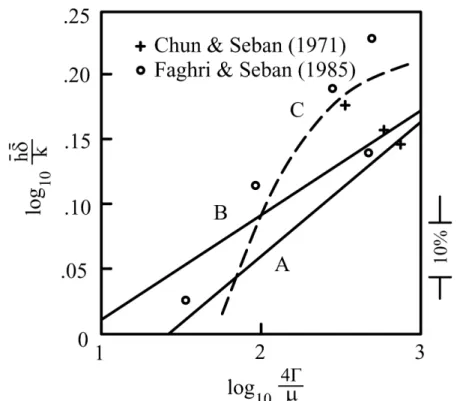
Figure 9.12 The average Nusselt number as a function of the Reynolds number: Curve A, Kutateladze (1982); Curve B, Kutateladze (1963);Curve C, Hirschburg and

 _{For practical purposes, Zozulja developed a correction for wavy laminar film}

based on condensation experiments (Stephen, 1994):

(9.150)

 _{An empirical correlation for the local heat transfer coefficient for}

laminar-wavy flow is obtained by combining eq. (9.150) with eq. (9.108),

(9.151)

 Empirical correlation for the onset of wavy laminar flow

(9.152)  _{Kapitza number} (9.153) Nusselt h h 11 . 0 4 Re 876 . 0 _      =

(

)

0.22 3 1 2 Re 828 . 0 − =       − g k h v ρ ρ ρ µ     1/11

Re Re

≥

_wavy

=

2.43

Ka

−

(

)

4 3 v

g

Ka

µ

ρ

ρ σ

=

−

l l

/ / w hh hh_δ / w hh / hh_δ



Empirical correlation of the average heat transfer

coefficient

(9.154)



Substituting eq. (9.109) into (9.154) an equation

correlating Re

_L

is obatined

(9.155)

(

)

(

(

)

)

_ _{1 3} 2 1.22 1.22

Re

Re

Re

Re

o L v o L

h

k

g

µ

ρ ρ

ρ





−

=



−



−





l l l l

(

)

(

)

1 3 1.22 1.22 0 ₂

Re

_L

Re

4

w v v v

k L T

T

g

h

ρ ρ

ρ

µ

µ





−

−

=

−









l l l l l l



Example 9.6

A uniformly-distributed liquid water film at 0.01 kg/s is

introduced at the top of a tube with an inner diameter of

4 cm and a height of 2 m. The inner surface temperature

of the tube is uniformly 105

°

C and the saturation

temperature of the steam is 100

°

C. Find the evaporation

rate and the average heat transfer coefficient.



Solution:

The properties of the liquid water and the steam can be approximated as those at the saturation temperature:

It is assumed that the liquid film thickness is much smaller than the radius of the tube. Therefore, the falling film analysis for evaporation over a vertical flat plate can be used.

The Kapitza number is obtained from eq. (9.153):

Therefore, the Reynolds number for wavy film is

o

0.68 W/m- C,

k

_l

=

3

958.77 kg/m ,

ρ

_l

=

2.79 10 N-s/m ,

4 2

58.9 10 N/m,

3 v

µ

=

×

−

σ

=

×

−

ρ

=

l 3 0.596 kg/m , hlv = 2251.2 kJ/kg.

(

)

4 4 4 13 3 3 3 (2.79 10 ) 9.8 3.032 10 (958.77 0.596) (58.9 10 ) v g Ka µ ρ ρ σ − − − × × = = = × − l − × × l 1/11 13 1/11 Re_wavy = 2.43Ka− = 2.43 (3.03 10 )× × − − = 33.4

 The inlet mass flow rate per unit perimeter is

 _{The Reynolds number at the inlet is}

which is also under the transition Reynolds number for turbulent,

. This means that the liquid film is in the laminar wavy regime.

 _{The Reynolds number at outlet can be obtained from eq. (9.155),}

i.e., 2 0 0 0.01 7.95 10 kg/s-m 0.04 m D π π − Γ = = = × × & 2 0 0 ₄ 4 4 7.95 10 Re 1139.8 Re 2.79 10 wavy µ − − Γ × × = = = > × l 1.05

Re

_turb

=

5840Pr

−

=

1862

(

)

(

)

(

)

1 3 1.22 1.22 0 ₂ 1 3 Re Re 4 958.77 958.77 0.596 9.8 w v v L fg k L T T g h ρ ρ ρ µ µ   − − = − _{ }    × − ×  × × − l l l l l

 Thus

which is still in the wavy regime so the entire surface is wavy.

 _{The mass flow rate of the liquid at the outlet is}

 The evaporation rate is therefore

 The heat transfer coefficient can be obtained from eq. (9.154), i.e.,

Re

_L

=

757.6

3 0 0 Re 757.6 0.01 6.64 10 Re 1139.8 L L m& = m& = × = × − 3 3 0

0.01 6.64 10

3.36 10

/

v L

m

&

=

m

&

−

m

&

=

−

×

−

=

×

−

kg m

(

)

(

)

(

)

1 3 _ 2 1.22 1.22 Re Re Re Re v o L o L g h k ρ ρ ρ µ  −  − = _{ } −   l l l l

(

)

1 3 4 2 1.22 1.22 958.77 958.77 0.596 9.8 1139.8 757.6 =0.68 (2.79 10 )− 1139.8 757.6  × − ×  − × _{ } × × −  

 _{Empirical relation between Reynolds and Prandtl numbers that can be used}

to determine turbulence for a falling film

(9.156)

 Momentum equation

(9.157)

 _{Defining the following dimensionless variables}

(9.158)

 _{The momentum equation becomes}

(9.159)

 _{Subject to the boundary conditions}

(9.160)

9.4.3 Turbulent Falling Film

05 . 1

Pr

5840

Re

≥

−

(

+

)

+

g

=

0

dy

du

v

dy

d

M

ε



,

,

o

u

_τ

=

τ ρ

_l

u

+

=

u u

_τ

y

+

=

yu v

_{τ l}

0

1

+

₃

=









+

₊+ + τ

ε

u

gv

dy

du

v

dy

d

_{M } 

0,

0

u

+

=

y

+

=

(9.161)

 Integrating eq. (9.159) twice and using eqs. (9.160) and (9.161) to

determine the integral constant, the dimensionless velocity becomes (9.162)

 Energy equation

(9.163)

 Subject to the boundary conditions

(9.164) (9.165) (9.166) 0, du y dy δ + + + + = =

(

)

(

)

0 1 1 y M y u dy v δ ε + + + + ₌ − + +

∫

l

(

)

y

T

y

x

T

u

_H

∂

∂

+

∂

∂

=

∂

∂

ε

α

0 sat T T= x = , 0 w q T y y k ′′ ∂ = − = ∂ _l , sat T T= y = δ

 _{Defining dimensionless temperature}

(9.167)

 Using dimensionless variables from eq. (9.158), the energy equation

becomes

(9.168)

 _{To predict heat transfer in falling film flow on a heat wall}

(9.169)

 _{Average heat tranfer coefficient can be obtained by subsitituting eq. (9.169)}

into eq. (9.112)

(9.170)

 For constant wall temperature the Reynolds number at x=L, Re_L is obtained

by substituting eq. (9.109) into eq. (9.170)

0 T cu T q τ

ρ

+ _{= l} + + + + +

∂

∂









+

∂

∂

=

∂

∂

y

T

v

v

y

x

T

u

H  

ε

α

(

)

1 3 2 3 0.4 0.65 3.8 10 Re Pr l v h k g µ ρ ρ ρ −   = ×  ₋    l l l

(

)

(

(

)

)

_ _{1 3} 2 3 0.65 0.6 0.6 Re Re 2.28 10 Pr Re Re o L v o L h k g µ ρ ρ ρ −   − = ×  ₋  ₋   l l l l

(

)

(

)

1 3



Assuming the shape of the droplet is hemispherical

during evaporation the energy balance at the interface

(9.172)



Simplified as

(9.173)



Scale of the temperature gradient at the interface

(9.174)



Scale analysis of eq. (9.173)

(9.175)

9.4.4 Surface Spray Cooling

(

)

/ 2 2 2 2 0

( , )

2

I I

2

cos

2

v I I I sat

dr

T r

h

r

k

r

d

h

r T

T

dt

r

π

θ

ρ

π

=

∂

π

θ θ

−

π

_∞

−

∂

∫

l l l l

(

)

/ 2 0

( , )

cos

I I v sat

dr

T r

h

k

d

h T

T

dt

r

π

θ

ρ

=

∂

θ θ

−

_∞

−

∂

∫

l l l l ( , )_{I w sat} i T T T r r R

θ

− ∂ ∂ :

(

)

i w sat

r

T

T

h

k

h T

T

ρ

:

−

+

−

 _{Eq. (9.175) can be rearranged as}

(9.176)

 _{Eq. (9.175) can be simplified by neglecting the second term on the}

right hand side

(9.177)

 _{The time it takes to completely evaporate the droplet with an initial}

radius of r_i is

(9.178)

 _{The scale of the heat flux at the heating surface}

(9.179)  _{Combining eqs. (9.178)-(9.179)} 2 ( ) ( ) v i i w sat sat f h r hr T T T T k t k ρ ∞ − + − l l l l : 2

(

)

i v w sat f

r

h

T

T

k t

ρ

_{l l}

−

l

:

(

)

2 v i f w sat

h r

t

k T

T

ρ

−

l l l

:

(

w sat

)

w i

k T

T

q

r

−

′′

:

l v i

h r

t

:

ρ

l l

 Conduction in the liquid droplet can be estimated by the following

correlation

(9.181)

 Average conduction area

(9.182)

 _{Average path length for conduction}

(9.183)

 _{Conduction in the liquid droplet becomes}

(9.184)

 _{The energy balance for the hemispherical droplet becomes}

(9.185) w sat d

T

T

q

k A

δ

−

=

_l 2

1

3

(

)

2

w I

2

I

A

=

A

+

A

=

π

r

3 2

(2 / 3)

4

(3/ 2)

9

I I I

r

V

r

A

r

π

δ

π

=

=

=

27

(

)

8

d I w sat

q

=

π

k r T

_l

−

T

2

27

2

(

)

8

I v I I w sat

dr

h

r

k r T

T

dt

ρ

_{l l}

π

=

π

_l

−



Rearranged as

(9.186)



Subjected to the following initial conditions

(9.187)



The transient radius of the droplet

(9.188)



Time required for the droplet to completely

evaporate

(9.189)

(

)

27

16

w sat I I v

k T

T

dr

r

dt

ρ

h

−

=

l l l

,

0

I i

r

=

r

t

=

2

27

(

)

8

w sat I i v

k T

T t

r

r

h

ρ

−

=

−

l l l 2

8

h r

_{v i}

t

=

ρ

l l



Example 9.7

A hemispherical liquid water droplet with an initial radius of

20 μm is attached to a heated wall and exposed to pure

water vapor at 1 atm. The temperature of the heated wall

is 180 °C. Estimate the time required for the liquid



Solution:

The saturation temperature corresponding to 1 atm is

T

_sat

=

100 °C. The properties of the liquid water can be

approximately evaluated at the saturation temperature:

The time required for the liquid droplet to evaporate

completely can be obtained from eq. (9.189) , i.e.,

o 0.68 W/m- C, k_l =

ρ =

_l

958.77 kg/m ,

3 h_lv = 2251.2 kJ/kg. 2 3 6 2 8 27 ( ) 8 958.77 2251.2 10 (20 10 ) 0.0047 s 4.7 ms 27 0.68 (180 100) v i f w sat h R t k T T ρ − = − × × × × × = = = × × − l l l

9.4.5 Evaporation on a Thin Liquid Film on the

Outer Surface of a Wedge or Cone Embedded

in a Porous Medium



Governing equation are

(9.190)

(9.191)

(9.192)

(9.193)

( )

r u

( )

r v ₀ x y ′′ ′′ ∂ ∂ + = ∂ ∂

( )

2

(

)

2 1 1 cos l v l l r u g u u p u vu u v v x y x x r x y K ρ ρ θ ρ ρ   ∂ ′′   − ∂ ₊ ∂ _{= −} ∂ ₊ ∂ ₊ ∂ _{− +}   _′′   ∂ ∂ ∂ _ ∂ _ ∂ _ ∂ _

( )

2

(

)

2 1 1 sin l v l l r v g v v p u vv u v v x y y x r x y K ρ ρ θ ρ ρ   ∂ ′′   − ∂ ₊ ∂ _{= −} ∂ ₊ ∂ ₊ ∂ _{− +}   _′′   ∂ ∂ ∂ _ ∂ _ ∂ _ ∂ _

( )

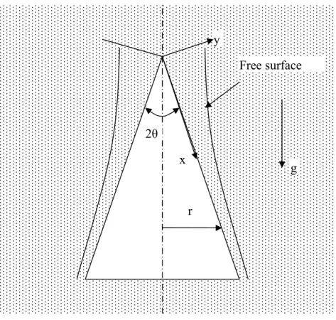
2 2 1 eff r u v x y x r x y φ φ φ   ∂ ′′  φ  ∂ ₊ ∂ _{= Γ} ∂ ₊ ∂   _′′   ∂ ∂ ∂ ∂ ∂

Figure 9.14 Film evaporation on surface of wedge or cone embedded in

y x r g 2θ Free surface



The effective thermal diffusivity

(9.194)



Mass diffusivity is

(9.195)



The governing equations (9.190)-(9.193) were

transformed to

(9.196)

(9.197)

(9.198)

(1

)

_s eff p

k

k

c

ε

ε

ε ρ

+ −

Γ

=

l l l eff Sc ν Γ = l 2 2

(

v

)cos

0

u

u

g

y

K

µ

µ

∂

−

+

ρ

−

ρ

θ

=

∂

l 0

(

v

) (

)sin

p

=

p

+

ρ

_l

−

ρ

g

δ

−

y

θ

2 2 eff

u

v

x

y

y

φ

φ

φ

∂

+

∂

= Γ

∂

∂

∂

∂

 Velocity distribution

(9.199) where

(9.200)

 Average film velocity was obtained by integrating the local velocity

across the film thickness

(9.201)

 Film thickness can be related to the velocity by satisfying the

conservation of mass at any x-location

(9.204) (9.205) where (9.206) * * cosh (1 ) 1 cosh D y u u δ δ +  −  = _ − _  

(

)

cos

D v

K

u

ρ

ρ

g

θ

µ

=

_l

−

l * * tan 1 D U u δ δ   = _ − _   * _tan * _A

δ

−

δ

= *₍ * _{tanh )}* 2 B x δ δ − δ = ₊ Q

(9.207)

(9.208)

(9.209)

3/ 2 2

2 sin

eff D

Q

B

K u

π

θ

Γ

=

2 eff

x

x

U

δ

+

=

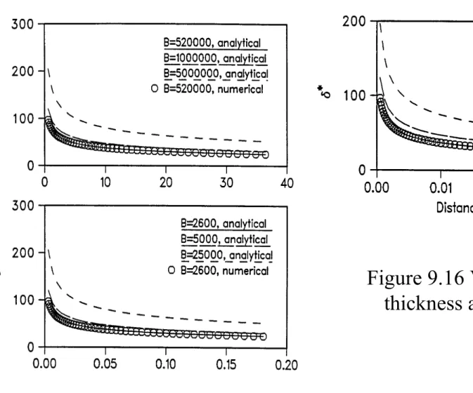
Γ

2 2 2 * * * * 2 For wedge: 1 1 For cone: 3 1 cosh( ) sinh( ) u x y u y u x x y y y y φ φ φ φ φ δ δ δ δ + + + + + + + + + + + + ∂ ₌ ∂ ∂ ∂   ∂ ∂ ∂  ₋  _{+ − =}    _{ ∂ − + ∂ ∂}   _{ }

Figure 9.16 Variation of film thickness along a wedge.