Multilevel techniques and learning automata for the Maximum Satisfiability (MAXSAT) problem

(1)

Multilevel Techniques and

Learning Automata for the

Maximum Satisfiability

(MAXSAT) Problem

By

Øystein Brådland

Mats G. L. Oseland

Supervisor

Associate Professor Noureddine Bouhmala, UiA/HiVe

This Master’s Thesis is carried out as a part of the education at the University of

Agder and is therefore approved as a part of this education. However, this does not

imply that the University answers for the methods that are used or the conclusions

that are drawn.

University of Agder, 2012

Faculty of Engineering and Science

(2)

Abstract

The Maximum Satisfiability (MAXSAT) Problem is a propositional logic and an

optimiza-tion based problem that has great importance in the theoretical and practical domain. In

the recent years MAXSAT has risen great interest in the industry. Example problems from

the industry that can be encoded as MAXSAT problems are circuit design and debugging,

hardware verification, bioinformatics and scheduling. These kind of problems often tend

to be large and increase exponentially with the problem size, and therefore algorithms for

solving such problems incorporate different techniques and methods to solve the problems

in a smart and efficient manner.

In this thesis we introduce a range of algorithms that extend the well-known Stochastic

Local Search (SLS) algorithm called

WalkSAT

.

WalkSAT

is extended with the multilevel

paradigm and Learning Automata. The multilevel paradigm is a technique that splits large

and difficult problems into smaller problems. These problems are expectedly less complex

and therefore easier to solve. Learning Automata are a branch of machine learning that

can be seen as a decision-making entity that is employed in an unknown environment.

Through feedback from the environment the Learning Automata try to learn the optimal

actions.

The core of this thesis is the observations and findings of how these dissimilar techniques

af-fect the performance and behaviour of

WalkSAT

when solving industrial MAXSAT problem

instances. Through extensive experiments our results confirm that combining multilevel

techniques and Learning Automata with

WalkSAT

, separately and together, give

promis-ing results. We compare these composite algorithms with

WalkSAT

on selected industrial

MAXSAT problems throughout the thesis, and show that all these composite algorithms

(3)

Acknowledgements

This master’s thesis is the final project in the master’s program in Information and

Com-munication Technology (ICT) at the University of Agder. The thesis has been under the

supervision of Associate Professor Noureddine Bouhmala.

We would like to thank Bouhmala for the valuable guidance and advices throughout the

work. This thesis would not have been possible without the help of Bouhmala through his

knowledge and insight in his field of research.

A paper entitled

Combining WalkSAT with Learning Automata for MAXSAT

is under

writing and will be submitted to a journal.

Grimstad, June 1, 2012

(4)

Contents

1

Introduction

1

1.1

Importance of topic and motivation . . . .

1

1.2

Thesis definition

. . . .

2

1.3

Research questions . . . .

2

1.4

Research approach . . . .

3

1.5

Contribution to knowledge . . . .

3

1.6

Limitations and key assumptions . . . .

3

1.7

Thesis outline . . . .

4

2

The Maximum Satisfiability Problem

5

2.1

Review of propositional logic

. . . .

5

2.2

Conjunctive normal form

. . . .

6

2.2.1

Transformation of propositional logic formulas to CNF . . . .

7

2.3

The Propositional Satisfiability Problem . . . .

8

2.4

The Maximum Satisfiability Problem . . . .

8

3

Solvers for MAXSAT

9

3.1

Algorithms for SAT and MAXSAT . . . .

9

3.1.1

Stochastic local search algorithms

. . . .

10

3.1.2

Systematic search algorithms . . . .

11

3.2

Solvers combined with Learning Automata . . . .

11

3.3

Solvers combined with multilevel techniques . . . .

11

3.4

Other prominent MAXSAT solvers . . . .

12

4

Experimental Design

13

4.1

Problem suite . . . .

13

4.2

Experiment setup . . . .

13

(5)

Experiment - benchmarking of multilevel WalkSAT . . . .

26

6.4.1

Results

. . . .

27

7

Combining WalkSAT with Learning Automata

32

7.1

Learning Automata and reinforcement learning . . . .

32

7.2

Learning Automata in a MAXSAT context

. . . .

33

7.3

Learning Automata WalkSAT . . . .

35

7.4

Experiment - Learning Automata state evaluation

. . . .

37

7.4.1

Results

. . . .

38

7.5

Experiment - benchmarking of

41

7.5.1

Results

. . . .

41

8

Combining WalkSAT with Multilevel Techniques and

Learning Automata

44

8.1

Multilevel Learning Automata WalkSAT . . . .

44

8.2

Experiment - benchmarking of

multilevel Learning Automata WalkSAT . . . .

45

8.2.1

Results

. . . .

45

9

Discussion

49

9.1

49

9.1.1

Wasting computational resources . . . .

49

(6)

CONTENTS

9.1.3

Single versus cluster . . . .

51

9.1.4

Static versus dynamic noise . . . .

51

9.2

51

9.3

Multilevel Learning Automata WalkSAT . . . .

51

9.4

Summary . . . .

52

10 Conclusion of the Research

53

10.1 Conclusion

. . . .

53

10.2 Further work . . . .

54

Bibliography

55

A Benchmarking Results

58

A.1 WalkSAT combined with multilevel techniques

. . . .

59

A.2 WalkSAT combined with Learning Automata . . . .

62

A.3 WalkSAT combined with multilevel techniques

and Learning Automata . . . .

64

(7)

List of Figures

1.1

The parts of the research approach. . . .

3

5.1

Problem instance fpu8-problem.dimacs_24.filtered.cnf, |variables| =160 232,

|clauses| = 548 848. Vertical axis gives the number of unsatisfied clauses,

horizontal axis represents the noise

p

.

. . . .

17

5.2

Problem instance wb1.dimacs.filtered.cnf, |variables| = 49 525, |clauses| =

140 091. Vertical axis gives the number of unsatisfied clauses, horizontal

axis represents the noise

p

. . . .

18

5.3

Problem instance 38584-bug-onevec-gate-0.dimacs.seq.filtered.cnf, |variables|

= 314 272, |clauses| = 819 830. Vertical axis gives the number of unsatisfied

clauses, horizontal axis represents the noise

p

. . . .

18

6.1

Clustering single objects. Single objects can be seen as one object when

clustered. . . .

20

6.2

Clustering and reduction of variables. |Variables| = 20, |variables per

clus-ter| = 2, |levels| = 3 (not counting level 0).

X

denotes a variable, and

c

denotes a cluster. . . .

21

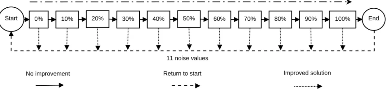
6.3

Dynamic noise procedure: 11 different noise values. Starts at 0%, ends at

100%, increments by 10%. The arrows specifies the possible transitions.

. .

24

6.4

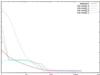
Log plot: Problem instance divider-problem.dimacs_3.filtered.cnf, |variables|

clauses, horizontal axis gives the time in seconds. . . .

27

6.5

Log plot: Problem instance dividers_multivec1.dimacs.filtered.cnf,

|vari-ables| = 106 128, |clauses| = 397 650. Vertical axis gives the number of

unsatisfied clauses, horizontal axis gives the time in seconds. . . .

27

6.6

Log plot: Problem instance i2c_master1.dimacs.filtered.cnf, |variables| =

82 429, |clauses| = 285 987. Vertical axis gives the number of unsatisfied

clauses, horizontal axis gives the time in seconds. . . .

28

6.7

Log plot: Problem instance rsdecoder1_blackbox_CSEEblock-problem.dimacs_32.

filtered.cnf, |variables| =277 950, |clauses| = 806 460. Vertical axis gives the

number of unsatisfied clauses, horizontal axis gives the time in seconds.

. .

28

(8)

LIST OF FIGURES

6.8

Log plot: Problem dividers_multivec1.dimacs.filtered.cnf, |variables| = 106

128, |clauses| = 397 650. Vertical axis gives the number of unsatisfied

clauses, horizontal axis gives the time in seconds. The vertical bars

indi-cate level transitions.

. . . .

29

6.9

Log plot: Problem instance spi2.dimacs.filtered.cnf, |variables| = 124 260,

horizontal axis gives the time in seconds. . . .

29

7.1

Interaction between an agent and its environment. . . .

32

7.2

Learning automaton states, actions, rewards and penalties, and their effects. 33

7.3

Left: Learning automaton state mirroring mechanism. Right: Learning

Au-tomata WalkSAT with one state per action. . . .

36

7.4

Problem instance divider-problem.dimacs_3.filtered.cnf. |variables| = 216

900, |clauses| = 711 249. Vertical axis gives the number of unsatisfied

clauses, horizontal axis gives the number of states per Learning

automa-ton.

. . . .

38

7.5

Problem instance fpu8-problem.dimacs_24.filtered.cnf. |variables| = 160

clauses, horizontal axis gives the number of states per Learning

automa-ton.

. . . .

38

7.6

Problem instance SM_RX_TOP.dimacs.filtered.cnf. |variables| = 235 456,

|clauses| =934 091. Vertical axis gives the number of unsatisfied clauses,

horizontal axis gives the number of states per Learning automaton. . . .

39

7.7

Log plot: Problem instance divider-problem.dimacs_3.filtered.cnf |variables|

41

7.8

Log plot: Problem instance dividers6_hack.dimacs.filtered.cnf |variables| =

42

7.9

Log plot: Problem instance spi2.dimacs.filtered.cnf |variables| = 124 260,

horizontal axis gives the time in seconds. . . .

42

8.1

Log plot: Problem instance divider-problem.dimacs_3.filtered.cnf |variables|

45

8.2

Log plot: Problem instance fpu8-problem.dimacs_24.filtered.cnf |variables|

46

8.3

Log plot: Problem instance dividers_multivec1.dimacs.filtered.cnf |variables|

=106 128, |clauses| = 397 650. Vertical axis gives the number of unsatisfied

46

(9)

LIST OF FIGURES

8.4

Log plot: Problem instance i2c_master1.dimacs.filtered.cnf |variables| =

clauses, horizontal axis gives the time in seconds. . . .

47

9.1

Log plot: Problem dividers_multivec1.dimacs.filtered.cnf, |variables| = 106

clauses, horizontal axis gives the time in seconds. The vertical bars

indi-cate level transitions.

. . . .

50

(10)

List of Tables

2.1

Truth tables for logical operations. . . .

6

2.2

Truth table for formula

g

. . . .

6

5.1

Problem instances used in the experiments, 9 in total. Listed with number

of variables and clauses. . . .

17

5.2

Industrial problem instances with the optimal noise for WalkSAT.

. . . . .

19

6.1

Multilevel WalkSAT variants and their differences. . . .

23

6.2

Problem instances used in the experiment, 20 in total. Listed with number

26

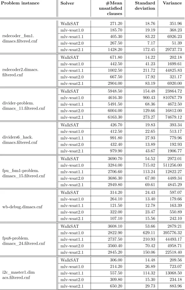
6.3

Results from the experiment. Multilevel WalkSAT variants and WalkSAT. .

31

7.1

Learning Automata WalkSAT variants and their differences. . . .

36

7.2

Problem instances used in the experiments, 8 in total. Listed with number

37

7.3

Results from the experiment. Problem instances given with optimal number

of states for both Learning Automata WalkSAT variants.

. . . .

39

7.4

Results from experiment. Learning Automata WalkSAT variants and

Walk-SAT. . . .

43

8.1

Multilevel Learning Automata WalkSAT building blocks.

. . . .

44

8.2

Results from experiment. Multilevel WalkSAT, Learning Automata

Walk-SAT, multilevel Learning Automata WalkSAT and WalkSAT. . . .

48

9.1

Multilevel consecutive reduction example. Contains levels, %PVA

(percent-age of possible variable assignments) and total amount of variables in a

hypothetical MAXSAT problem with 100 variables at level 0. Note that we

have 2 variables per cluster. . . .

50

A.1 Results from benchmarking. Multilevel WalkSAT variants and WalkSAT.

.

59

A.2 Results from benchmarking. Multilevel WalkSAT variants and WalkSAT.

.

60

(11)

LIST OF TABLES

A.4 Results from benchmarking. Learning Automata WalkSAT variants and

WalkSAT. . . .

62

A.5 Results from benchmarking. Learning Automata WalkSAT variants and

WalkSAT. . . .

63

A.6 Results from benchmarking. Multilevel WalkSAT, Learning Automata

64

A.7 Results from benchmarking. Multilevel WalkSAT, Learning Automata

65

A.8 Results from benchmarking. Multilevel WalkSAT, Learning Automata

(12)

List of Algorithms

1

SAT-SLS

. . . .

10

2

WalkSAT architecture . . . .

14

3

WalkSAT . . . .

15

4

The multilevel paradigm . . . .

22

5

23

(13)

List of Definitions

1

Thesis definition . . . .

2

Satisfiability . . . .

7

3

The SAT problem

. . . .

8

4

The unweighted MAXSAT problem . . . .

8

5

Break-count . . . .

15

6

Cluster flip . . . .

24

7

Multilevel-multiplier . . . .

24

(14)

Chapter 1

Introduction

In this chapter we briefly put forward the Maximum Satisfiability Problem (MAXSAT).

We introduce the problem area, its importance, and our motivation behind this research

in section 1.1. The thesis definition is given in section 1.2, research questions based on

the definition are formed in section 1.3. The steps of conducting our research are given

in section 1.4. We highlight our contribution to knowledge in section 1.5 followed by

limitations and key assumptions in section 1.6. The chapter ends with an outline of the

thesis in section 1.7.

1.1

Importance of topic and motivation

Research on solving MAXSAT has great importance. It is mainly important because there

are many theoretical and practical problems that can be encoded as MAXSAT problems.

Circuit design and debugging, scheduling of how an observation satellite captures photos of

Earth, and protein structure alignment (bioinformatics) are all applications and problems

from the industry that can be translated to MAXSAT [1–3].

MAXSAT is the optimization variant of the propositional satisfiability problem known

as SAT. Due to the MAXSAT problem’s structure, the complexity grows exponentially

depending on the problem size, hence the time it would take to test all the different

solutions could easily be too long. In order to solve a MAXSAT problem efficiently, it is

not sufficient to have a fast implementation, but also to be able to move around in the

search space in an intelligent manner using various methods and techniques. By doing so, a

large number of solutions will be visited and evaluated, thereby increasing the probability

for reaching the best possible solution. Hence, the solver will perform more efficiently.

Another important factor for researching on MAXSAT solvers is that if there is a MAXSAT

problem, it can be solved by any MAXSAT solver

1

. However, some solvers might work

better on specific problem types, and worse on others. It is therefore important to have

this in mind when developing a MAXSAT solver.

Stochastic Local Search (SLS) algorithms are known to perform well on SAT problems

[4–6]. Therefore, it is interesting to see if it is possible to enhance the performance of SLS

algorithms by applying various techniques for solving MAXSAT. Extending an existing

SLS algorithm is the integral part of our research, with the goal being that it will be able

to solve MAXSAT problems in a more efficient manner. Our research will focus on an

1

Any MAXSAT problem can essentially be solved by any MAXSAT solver, assuming the problem format is supported.

(15)

CHAPTER 1. INTRODUCTION

algorithm called

WalkSAT

that will be combined with Learning Automata and multilevel

techniques. We then explore the effects of extending

WalkSAT

with the aforementioned

methods. Especially, we want to compare the performance of

WalkSAT

to our proposed

extensions of

WalkSAT

on industrial MAXSAT problem instances.

1.2

Thesis definition

Our thesis definition is given below.

Definition 1

Thesis definition: The MAXSAT problem is known to be NP-hard and

is an optimization variant of the SAT problem. The performance of many optimization

techniques deteriorates very rapidly mostly due to two reasons. First, the complexity

of the problem usually increases with its size, and second, the solution space of the

problem increases exponentially with the problem size. Therefore it is beneficial for

MAXSAT solvers to move around in the solution space in a smart and efficient

man-ner to reach the optimal or the best possible solution. In the paper A Multilevel Memetic

Algorithm for Large SAT-Encoded Problems, Bouhmala proposes a multilevel approach

for solving bounded model checking problems. In Using Learning Automata to Enhance

Local-Search Based SAT Solvers with Learning Capability by Granmo and Bouhmala,

they introduce a novel approach of using machine learning in a SAT context. Results

from the multilevel and machine learning methods proved to be promising. The purpose

of this master thesis is to see whether combining state of the art stochastic local search

methods with multilevel-techniques and Learning Automata for solving MAXSAT

re-sults in better performance.

1.3

Research questions

Based on the thesis definition we establish four research questions. These questions will

function as our main objectives. They are important subjects of the study that we will

answer by the end of this work.

1.

Learning Automata and multilevel techniques combined with other SAT

solvers have recently been used to solve SAT. What will be the outcome

when

WalkSAT

is extended with the aforementioned techniques for solving

MAXSAT?

Previous successful research shows that Learning Automata paired with

GSATRW and RW [7], and multilevel techniques paired with a memetic algorithm [8]

for solving SAT problems gave great improvement. However, it is not hereby given

that the results will be the same for MAXSAT problems. Further, SLS solvers that

perform well in SAT does not necessarily perform equally well in MAXSAT [1].

It might be the case that the structure and semantics of

WalkSAT

will increase or

decrease the significance of Learning Automata and multilevel techniques.

2.

Assuming we experiment with different combinations of

WalkSAT

with

mul-tilevel techniques, and

WalkSAT

with Learning Automata. What is the

op-timal combination in both aspects?

WalkSAT’s

structure opens for a degree of

freedom for extension. How the combination is done may play an important role. We

will therefore experiment with different combinations.

3.

If

WalkSAT

extended with Learning Automata and multilevel techniques

separately yields good results, what will be the result of

WalkSAT

combined

(16)

CHAPTER 1. INTRODUCTION

with both techniques?

The two techniques differs from each other, and it might

be the case that one of the two will boost the other to achieve an overall higher

performance when combined.

4.

Is there an optimal configuration of Learning Automata when coupled

with

WalkSAT?

A Learning automaton is a kind of a finite state machine that can be

configured in several ways. The number of internal states can affect the performance.

1.4

Research approach

In order to achieve the goals of this thesis the research is divided into four parts. Figure

1.1 illustrates the research approach and the four parts. First, we implement the original

version of

WalkSAT

, second, we combine multilevel techniques with

WalkSAT

. In the third

part we combine Learning Automata and

WalkSAT

. Finally, we combine both multilevel

techniques and Learning Automata with

WalkSAT

at the same time.

WalkSAT WalkSAT WalkSAT Learning Automata 1 2 3 4 WalkSAT Multilevel techniques Multilevel techniques Learning Automata

Figure 1.1: The parts of the research approach.

In all parts we perform experiments and compare our proposed algorithms with each other

and with

WalkSAT

. Findings from part 2 and 3 will be used as a basis for part 4.

1.5

Contribution to knowledge

The main contribution of our research will be the combination of the well-known stochastic

local search algorithm

WalkSAT

with multilevel techniques and Learning Automata. It will

provide valuable information on how multilevel techniques and Learning Automata affect

the performance of

WalkSAT

. Additionally, this research will function as a foundation and

reference point for possible future work.

1.6

Limitations and key assumptions

All the implemented algorithms presented in this thesis are not to be seen as complete

algorithms that can serve as final products. They are rather unoptimized prototypes of

what can be, and at this stage they only satisfy our needs required to complete and

pursue the goals of this thesis. Hence the results displayed in tables and graphs might

not correspond to optimized versions. Due to this, the results are not to be compared

(17)

CHAPTER 1. INTRODUCTION

with competing solvers from MAXSAT competitions and evaluations where computational

speed plays an important role.

1.7

Thesis outline

The remainder of the paper is organized as follows: Chapter 2 holds the problem area of

this research, namely the MAXSAT problem. In chapter 3 we present methods for solving

MAXSAT, and we also introduce prior research with emphasis on Learning Automata and

multilevel techniques for SAT. Notes on experimental design are put forward in chapter 4.

In chapter 5 the

WalkSAT

algorithm is set forth and examined in-depth. Chapter 6 contains

WalkSAT

combined with multilevel techniques, and in chapter 7

WalkSAT

is combined with

Learning Automata. We present

WalkSAT

combined with both multilevel techniques and

Learning Automata in chapter 8. Then, in chapter 9 we discuss results and observations

found from all experiments we have performed in chapter 6, 7 and 8. Finally, we conclude

our research and introduce possible further work in chapter 10.

(18)

Chapter 2

The Maximum Satisfiability

Problem

In this chapter we present the Maximum Satisfiability (MAXSAT) Problem. The chapter

comprises preliminary background information that helps the reader get acquainted with

MAXSAT.

We start by introducing propositional logic in section 2.1, which is the core structure

of a MAXSAT problem. In section 2.2 we show how propositional logic formulas can be

transformed into a form called CNF, which is used as input for many SAT and MAXSAT

solvers. We then turn the attention to MAXSAT. Due to the close relationship between

SAT and MAXSAT, we first introduce SAT in section 2.3, and then we introduce MAXSAT

in section 2.4. These sections also point out applications and definitions.

2.1

Review of propositional logic

Propositional logic is a system where the interest lies within propositions and their

inter-relationships. A proposition is a statement that can be assigned two values, either

T RU E

or

F ALSE

, also equivalent to 1 and 0, hereafter known as truth values. The logical

op-erations, also known as connectives, include

∨

(OR and logical disjunction),

∧

(AND and

logical conjunction),

¬

(NOT and logical negation),

→

(implication), and

↔

(equivalence).

These can be applied on two propositions, but

¬

can only be applied on one proposition.

When applied, the outcome is another proposition.

A formula with propositions can be evaluated as

T RU E

or

F ALSE

. Examples of

proposi-tions from real life are

x

1

=

It is

−

5

degrees Celsius outside today in Grimstad

, and

x

2

=

I

will wear my scarf and mittens today

. These propositions are primitive propositions which

can be combined to a compound proposition by using logical conjunction:

It is

−

5

degrees

Celsius outside today in Grimstad

, AND

I will wear my scarf and mittens today

. With

symbols this can be expressed as (

x

1

∧

x

2

).

A truth table is used to show the semantics for a logical operation. Table 2.1 gives the

truth tables for the mentioned logical operations.

(19)

CHAPTER 2. THE MAXIMUM SATISFIABILITY PROBLEM

X Y X∨Y X∧Y ¬X X↔Y X→Y 0 0 0 0 1 1 1 1 0 1 0 0 0 0 0 1 1 0 1 0 1 1 1 1 1 0 1 1

Table 2.1: Truth tables for logical operations.

An example of a propositional logic formula

g

with propositions, or variables,

x

1

, x

2

, x

3

,

and

x

4

is given below.

g

= (

¬

x

1

∨

(

¬

x

2

→

x

3

))

↔

x

4

(2.1)

The truth table for this formula is given in table 2.2. Each entry in the table shows the

truth values

x

1

, x

2

, x

3

, and

x

4

take to evaluate

g

as

T RU E/

1 or

F ALSE/

0. This can be

observed in the rightmost column.

x1 x2 x3 x4 g 1 1 1 1 1 1 1 1 0 0 1 1 0 1 1 1 1 0 0 0 1 0 1 1 1 1 0 1 0 0 1 0 0 1 0 1 0 0 0 1 0 1 1 1 1 0 1 1 0 0 0 1 0 1 1 0 1 0 0 0 0 0 1 1 1 0 0 1 0 0 0 0 0 1 1 0 0 0 0 0

Table 2.2: Truth table for formulag.

2.2

Conjunctive normal form

A possible encoding form for propositional logic formulas is the Conjunctive Normal Form

(CNF). This form is widely used for describing SAT and MAXSAT problems. A CNF

formula consists of a conjunction of clauses,

V

i

C

i

. Each clause

C

i

is a disjunction of

literals,

W

j

x

i,j

, where a literal is a propositional variable

x

(

T RU E

or

F ALSE

) or its

negation

¬

x

[9]. A CNF formula can be expressed as in equation 2.2 and 2.3, where

m

is

the number of clauses and

x

is a literal in a given clause. Equation 2.4 shows an instance

of a CNF formula with four variables

x

1

, x

2

, x

3

, x

4

and four clauses.

(20)

CHAPTER 2. THE MAXIMUM SATISFIABILITY PROBLEM

f

=

m ^ i=1

C

i

(2.2)

C

i

=

ki _ j=1

x

i,j

(2.3)

f

= (

x

1

∨

x

4

)

∧

(

¬

x

2

∨

x

4

)

∧

(

¬

x

3

∨

x

4

)

∧

(

¬

x

4

∨ ¬

x

1

∨

x

2

∨

x

3

)

(2.4)

A formula expressed in CNF is satisfied if all its clauses are satisfied, i.e. all clauses evaluate

to

T RU E

. For a clause to be satisfied at least one of the literals must evaluate to

T RU E

,

because of the disjunctions of literals. In formula 2.4 there are four variables

x

1

,

x

2

,

x

3

and

x

4

, which means there are 2

4

= 16 possible variable assignments of truth values. On the

other hand, if the formula has 500 variables then there are 3

.

27339061

×

10

150

assignments.

In a SAT/MAXSAT context these possible variable assignments are referred to as the

search space. One of the assignments of equation 2.4, where

x

1

=

T RU E

,

x

2

=

F ALSE

,

x

3

=

T RU E

,

x

4

=

T RU E

, makes

f

evaluate to

T RU E

. Hence, this assignment is called

a solution. This can also be seen from the truth table for the formula

g

(table above),

table 2.2 and equation 2.1. Since

g

can be transformed into CNF yielding

f

, the table is

also valid for

f

. The table reports that there exists eight solutions, eight rows where the

rightmost column holds the value 1 (the rows that are colored gray). Based on this we

define

satisfiability

in respect to propositional logic as following:

Definition 2

Satisfiability: Given a propositional formula

f

. If an assignment of truth

values to the variables in

f

evaluates

f

to

T RU E

, the assignment

satisfies

f

. Further,

f

is claimed to be

satisfiable

if and only if there exists at least one assignment that

satisfies

f

[6].

According to definition 2 we can claim that formula

f

is satisfiable since there is at least one

assignment of truth values that satisfies the formula, thus makes the formula satisfiable.

2.2.1

Transformation of propositional logic formulas to CNF

The main idea behind transforming a propositional logic formula to CNF is by using

logic transformation rules, where the goal is to create clauses with literals by only using

the logical connectives

∧

,

∨

and

¬

. The listing below shows how the propositional logic

formula

g

given in equation 2.1 can be transformed into CNF by using De Morgan’s law,

double negative law and the distributive law. We also need to decompose the connective

double implication

↔

: (

x

1

↔

x

2

)

⇔

(

x

1

→

x

2

)

∧

(

x

2

→

x

1

), and the logical connective

implication

→

: (

x

1

→

x

2

)

⇔

(

¬

x

1

∨

x

2

) [10].

(

¬

x

1

∨

(

¬

x

2

→

x

3

))

↔

x

4

⇔

((

¬

x

1

∨

(

¬

x

2

→

x

3

))

→

x

4

)

∧

(

x

4

→

(

¬

x

1

∨

(

¬

x

2

→

x

3

)))

⇔

(

¬

(

¬

x

1

∨

(

¬

x

2

→

x

3

) )

∨

x

4

)

∧

(

¬

x

4

∨

(

¬

x

1

∨

(

¬

x

2

→

x

3

)))

⇔

(

¬

(

¬

x

1

∨

(

x

2

∨

x

3

) )

∨

x

4

)

∧

(

¬

x

4

∨

(

¬

x

1

∨

(

x

2

∨

x

3

)))

⇔

((

x

1

∧ ¬

(

x

2

∨

x

3

) )

∨

x

4

)

∧

(

¬

x

4

∨

(

¬

x

1

∨

(

x

2

∨

x

3

)))

⇔

((

x

1

∧

(

¬

x

2

∧ ¬

x

3

))

∨

x

4

)

∧

(

¬

x

4

∨

(

¬

x

1

∨

(

x

2

∨

x

3

)))

(21)

CHAPTER 2. THE MAXIMUM SATISFIABILITY PROBLEM

⇔

((

x

1

∧ ¬

x

2

∧ ¬

x

3

)

∨

x

4

)

∧

(

¬

x

4

∨ ¬

x

1

∨

x

2

∨

x

3

)

⇔

(

x

1

∨

x

4

)

∧

(

¬

x

2

∨

x

4

)

∧

(

¬

x

3

∨

x

4

)

∧

(

¬

x

4

∨ ¬

x

1

∨

x

2

∨

x

3

)

The expression in the last line in the listing above is the same as given in equation 2.1,

hence the propositional logic formula has been transformed into CNF. As can be seen

from the final result, negation (

¬

) now only appears on single literals inside clauses. The

only logic connectives left are

∧

and

∨

, and all the occurrences of

↔

and

→

have been

decomposed.

2.3

The Propositional Satisfiability Problem

The Propositional Satisfiability Problem, also known as the SAT problem, is essential

in mathematical logic and computing theory, but it also has interests in applications

belonging to the practical domain. As can be understood from the name, the structure of

the SAT problem builds on the propositional logic presented in the previous sections.

Real-world problems and applications include Blocks World (planning problem in the AI

domain), graph coloring, circuit design and hardware verification can all be encoded as

SAT problems [1]. The SAT problem is under the NP-complete class of problems [9], and

the goal is to determine whether there exists an assignment of truth values to the variables

in a given CNF formula such that it becomes satisfiable [6]. We define the SAT problem

as following:

Definition 3

The SAT problem: Given a propositional formula

f

, does there exist an

assignment of truth values to the variables such that

f

becomes satisfiable?

2.4

The Maximum Satisfiability Problem

The Maximum Satisfiability (MAXSAT) Problem is an optimization variant of the SAT

problem. The complexity of such problems is known to be NP-hard [9]. Applications and

problems from the industry involve bioinformatics [3], scheduling [2] and integrated circuits

such as field-programmable gate array (FPGA) routing [11].

MAXSAT has several variants: the weighted MAXSAT problem, the unweighted MAXSAT

problem, the partial MAXSAT problem and the weighted partial MAXSAT problem [12].

In the weighted variants each clause in a problem has an associated weight, and where

the goal is to maximize the total weight of the satisfied clauses. For unweighted MAXSAT

the goal is to minimize the amount of unsatisfied clauses

1

in a given CNF formula [6]. We

define the unweighted MAXSAT problem as following:

Definition 4

The unweighted MAXSAT problem: Given a propositional formula

f

,

does there exist an assignment of truth values to the variables that maximizes the

number of satisfied clauses in

f

?

The difference between SAT and MAXSAT is now evident according to definition 3 and

4: SAT is a decision based problem, while MAXSAT is an optimization based problem.

Our focus lies on unweighted MAXSAT, and therefore for the rest of this thesis the term

MAXSAT refers to unweighted MAXSAT.

1

(22)

Chapter 3

Solvers for MAXSAT

This chapter comprises methods for solving MAXSAT and introduces prior significant

work for solving SAT through the employment of multilevel techniques, and algorithms

with learning capabilities. We also present a selection of MAXSAT solvers.

An introduction to SAT and MAXSAT solvers is given in section 3.1, where the two main

branches of solvers, stochastic local search algorithms and systematic search algorithms,

are discussed in more detail in section 3.1.2 and 3.1.1. Since stochastic local search

algo-rithms is our main focus we provide more information on this subject.

Section 3.2 introduces prior work where various stochastic local search algorithms have

been paired with Learning Automata. A memetic algorithm and an algorithm called

GSAT

combined with multilevel techniques are set forth in section 3.3. The chapter ends with

section 3.4 that contains a brief overview of prominent MAXSAT solvers.

3.1

Algorithms for SAT and MAXSAT

SAT and MAXSAT solvers, or algorithms, are used to solve propositional problem

in-stances. Due to the definitions of SAT and MAXSAT the goals for these solvers are

dif-ferent, see definition 3 and 4. The goal for a SAT solver is to achieve satisfiability for a

given problem. However, a MAXSAT solver seeks to maximize the amount of satisfied

clauses. Hence, it might not solve all clauses, but the problem might be satisfied according

to given constraints. The goals are realized by

flipping

variables in the problem, where

flipping means to negate the truth value of a variable.

As we pointed out in section 2.2, a propositional formula that consists of 500 variables

has 3

.

27339061

×

10

150

different variable assignments. This illustrates the magnitude of

dealing with propositional logic formulas with a high number of variables. It is therefore

clear that solvers need to be designed efficiently to obtain good coverage of the search

space and find optimal solutions within reasonable time.

Solvers are generally divided into two branches: Stochastic local search algorithms, and

systematic search algorithms. The two types of solvers are discussed in more detail in the

next sections.

(23)

CHAPTER 3. SOLVERS FOR MAXSAT

3.1.1

Stochastic local search algorithms

Solvers that are based on Stochastic Local Search (SLS) are often said to be incomplete.

An incomplete solver does not guarantee that it will provide a satisfying assignment, or

claim that the problem instance is unsatisfiable. Most of the solvers are concerned with

reporting satisfying assignments, if there exists one. Incomplete algorithms often run until

a constraint has been met, e.g. a time limit, max amount of flips or other such properties.

Systematic search algorithms used to dominate the field of solving large SAT problem

instances. However, in the 1990’s stochastic local search algorithms proved its strength

for solving large and hard SAT problems [13]. Two of the most important solvers among

incomplete solvers that paved the way for SLS algorithms for SAT were

GSAT

[5] and

WalkSAT

[4].

GSAT

was one of the first SLS SAT solvers presented in 1992 and

WalkSAT

was introduced in 1994 which originated from

GSAT

with slight modifications.

The strength and approach for SLS algorithms are the usage of local information. With

this approach SLS algorithms are able to find good solutions without exploring the entire

search space. They start by examining the search space at some position and then move

to a position nearby. From the latter position the decision about the next move is decided

by the information from the local neighborhood, where the neighborhood can be seen as

a variable assignment. The search is stochastic in the sense that the decisions and moves

can be based on stochastic properties. On the other hand, one of the weaknesses of SLS

algorithm is that they can get stuck in a state known as local minima

1

. There are several

suggested ways to deal with this issue. Restart

2

and non-improving steps are common

mechanisms used in many algorithms [14].

In most cases SLS algorithms have an associated objective function. The objective function

is often denoted as the number of unsatisfied clauses under a given assignment.

Conse-quently, SLS algorithms try to minimize this function [14]. In general, each variable

x

in

a given problem has a score associated with it, in respect to an assignment. There are

different scoring functions of measuring this score, depending on the algorithm (e.g.

GSAT

,

WalkSAT

or other SLS algorithms).

Algorithm 1

SAT-SLS

1:

{

Input:

CNF formula G}

2:

{

Output:

Satisfied assignment for G, or ’no solution exists’}

3:

for

i

←

0 to MAX_TRIES

do

4:

T

←

random_assignment()

5:

for

j

←

0 to MAX_FLIPS

do

6:

if

T is satisfied

then

7:

return

T

8:

else

9:

/* heuristics */

10:

variable

←

select

_

variable

()

11:

end if

12:

flip(variable)

13:

end for

14:

end for

1

A local minimum is a point in the search space where the local neighborhood does not have a point that is better (i.e. lower number of unsatisfied clauses).

2

(24)

In algorithm 1 above (reproduced from [15]) a generic outline of SLS algorithms for SAT is

given. In the initialization phase all the variables in a given formula are randomly assigned a

truth value. Then the algorithm selects a variable and flips its. This is done in an iterative

process and can also be seen as a trial and error approach. The heuristics of variable

selection is what changes from one SLS algorithm to another. The selection is often done

according to the scoring function, and has significant impact on the overall performance [6].

Further, according to algorithm 1 the SLS algorithm will repeat selecting variables and

doing flips until MAX_FLIPS is reached. If no solution is found, the algorithm restarts

with a new random assignment. The algorithm stops executing when it has reached a

predefined number of allowed restarts denoted as MAX_TRIES.

The algorithm presented in the outline is for solving SAT problems, but it is also valid for

MAXSAT with minor modifications. Generally, all SLS algorithms can be modified and

adapted to solve unweighted MAXSAT problems. However, this does not imply that SLS

solvers performing well in SAT yield the same performance in MAXSAT [6].

3.1.2

Systematic search algorithms

Solvers that are classified as systematic search algorithms are known as complete solvers.

In comparison to incomplete solvers complete solvers are guaranteed to find a satisfying

assignment if one exists, or prove unsatisfiability. Hence, systematic search algorithms

search the entire solution space (all possible variable assignments) of the given problem.

Because of this complete solvers may be more computationally expensive, and have often

difficulties solving large problems.

Many of the complete solvers are based on

DPLL

[16] that was introduced in 1962, which

is also based on the

DP

[17] algorithm from 1960.

DPLL

builds a binary tree by assigning

truth values to variables, and uses backtracking and branching as its main components.

Successful algorithms based on

DPLL/DP

are

GRASP

[18],

SATO

[19],

TABLEAU

[20] and

SATZ

[21].

3.2

Solvers combined with Learning Automata

Previous work in the field of SAT solvers and machine learning have shown that mixing

(stochastic) local search SAT algorithms with Learning Automata has given promising

results. The goal is to let a SAT solver learn and decide what steps are the best ones to

achive better performance than without learning. The machine learning technique that has

been used by Granmo and Bouhmala was a Tsetlin automaton. Granmo and Bouhmala’s

work on fusing Learning Automata (LA) with both

Random Walk

[22] and

GSATRW

[22],

giving

LARW

and

LA-GSATRW

respectively, had a higher success rate and better performance

than their non-LA counterparts on selected problems from the SATLIB benchmarks in [23].

3.3

Solvers combined with multilevel techniques

Bouhmala proposed the multilevel memetic algorithm

MLVLMA

in [8] for solving large SAT

Bounded Model Checking problem instances. His research shows how a memetic algorithm

3

can utilize the multilevel paradigm. The multilevel paradigm is a method for splitting large

3

(25)

and difficult problems into smaller problems. These problems are expectedly less complex

and therefore easier to solve. The results show that combining a memetic algorithm with

the multilevel paradigm can improve the quality of the solution up to 77% in some cases.

In [25] the multilevel paradigm is combined with the stochastic local search algorithm

GSAT

. Conclusions drawn from the results indicate that the multilevel paradigm speeds up

GSAT

and improves its convergence.

3.4

Other prominent MAXSAT solvers

Solvers that distinguished themselves in the Max-SAT Evaluation 2006

4

are

MAXSATZ

[27]

and

MAX-DPLL

[28]. The former was the best unweighted MAXSAT solver, and the latter

was pointed out as the best solver for weighted MAXSAT.

MAX-DPLL

was also announced

as the second best unweighted solver [29, 30].

Other algorithms related to our work that are based on SLS for solving MAXSAT are

SAPS

[31] and

DLS-MC

[32]. Both of these algorithms use a technique called Dynamic

Local Search (DLS). DLS is used to avoid getting stuck in local minima. This is done by

dynamically altering the evaluation function of solutions at run time. Further, DLS allows

the search space to be dynamically changed and modified, thus the solver is guided to

avoid local minima.

4

The MAXSAT Evaluation [26] is an affiliated event of International Conferences on Theory and

(26)

Chapter 4

Experimental Design

In this chapter we give general information on how the experiments and benchmarking of

algorithms have been performed. We present the problem suite in section 4.1. Information

about the setup of the experiments is given in section 4.2, and in section 4.3 we report notes

on the algorithms’ implementation, and system specifications for our test environment.

4.1

Problem suite

In our experiments and benchmarks we use a selection of the same problems as used in

the MAXSAT Evaluations. All the problems follow the DIMACS CNF file format [33]. We

are focusing on industrial problems, and all of these are available at MAXSAT Evaluation

websites found at http://www.maxsat.udl.cat/. Our problem suite is a mixture of the

problems used in MAXSAT Evaluation 2008, 2009, 2010 and 2011.

4.2

Experiment setup

All the algorithms run 10 times on the same problem instance due the random nature in

stochastic local search algorithms. We calculate the mean results from these 10 times to

get an overview of how the algorithms perform in general. These mean results are used as

a basis for all the graphs and numbers in tables occurring in this thesis. In addition, all the

algorithms have an execution duration of

x

seconds, or

y

flips. When presenting figures,

graphs and tables we use the notation |.| for size (e.g. |clauses| = 4), and # for "number

of" (e.g. #Unsatisfied clauses equals "number of Unsatisfied clauses"). We also use graphs

in logarithmic and arithmetic scale to visualize data and results. For some results we also

give sample variance and sample standard deviation.

4.3

Implementation and machine specifications

All algorithms have been implemented by using the

C++

programming language, and run

on a machine with the following specifications:

• Central processing unit (CPU): 2x Intel Xeon Six Core E5645 2.4 GHz with 12 MB Cache

• Memory (RAM): 24 GB DDR

(27)

Chapter 5

WalkSAT

In chapter 3 we introduced methods for solving the MAXSAT problem. We especially focused on the branch called stochastic local search algorithms. In this chapter we take a closer look at the algorithm calledWalkSAT.

Introduction to the WalkSAT family is given in section 5.1, while in section 5.2 we introduce

WalkSAT/SKC which is our focus in this thesis. In section 5.3 we point out the implementation of this algorithm, and in section 5.4 we present results from noise evaluation.

5.1

The WalkSAT family

TheWalkSATfamily, often referred to as an architecture, is a collective term for successful stochastic local search algorithms for solving propositional logic problems. There exists a great amount of

WalkSATvariants such asWalkSAT/SKC,Novelty,Novelty+,Adaptive Novelty+,R-noveltyand

Walk-SAT/Tabu[6]. Nonetheless, all the variants have the same basis for variable selection and is done in two stages: In stage one a currently unsatisfied clause is picked at random.

Algorithm 2

WalkSAT architecture

1:

{

Input:

CNF formula G}

2:

{

Output:

3:

for

i

←

0 to MAX_TRIES

do

4:

T

←

random_assignment()

5:

for

j

←

0 to MAX_FLIPS

do

6:

if

T is satisfied

then

7:

return

T

8:

end if

9:

/* stage 1*/

10:

C

k

←

random_unsatisfied_clause()

11:

/* stage 2*/

12:

variable

←

random

_

variable

(

C

k

)

13:

flip(variable)

14:

end for

15:

end for

In stage two a variable that occurs in the unsatisfied clause is chosen at random. A generic outline of theWalkSAT architecture is given in algorithm 2. The main difference between all variants is how the variable is selected, as we will see in the next section. Due to this two-stage process, we observe that WalkSAT has 2-way randomness built in. In addition, these algorithms incorporate

(28)

CHAPTER 5. WALKSAT

randomized behaviour, such that during the execution they will perform a random move according to a given probability on how to select a variable. This probability is the so-called noise parameter. As with any other stochastic local search algorithms, the noise parameter is also one of the key elements that influences the performance for allWalkSATvariants.

5.2

WalkSAT/SKC

TheWalkSAT/SKC [4] algorithm was introduced by Selman, Kautz, and Cohen in 1994. It was the first algorithm belonging to theWalkSATarchitecture, and is the algorithm of interest in our thesis. For simplicity, we will for the rest of this paper refer toWalkSAT/SKC asWalkSAT.

As stated earlier, SLS algorithms and variants ofWalkSATmainly differ in the variable selection.

WalkSATcontains three moves for variable selection: (1) a side move/best move, (2) a greedy move, and (3) a random move. The pseudo code forWalkSATis given in algorithm 3.

Algorithm 3

WalkSAT

1:

{

Input:

CNF formula G}

2:

{

Output:

3:

Initialization:

p

noise

∈

[0, 1]

4:

for

i

←

0 to MAX_TRIES

do

5:

T

←

random_assignment

6:

for

j

←

0 to MAX_FLIPS

do

7:

if

T is satisfied

then

8:

return

T

9:

end if

10:

C

k

←

random_unsatisfied_clause()

11:

/* best move/side move */

12:

if

∃

variable

v

∈

C

k

with break-count = 0

then

13:

variable

←

v

14:

else

15:

if

random(0, 1)

< p

noise

then

16:

/* random move*/

17:

variable

←

random

_

variable

(

C

k

)

18:

else

19:

/* greedy move*/

20:

variable

←

random

_

lowest

_

breakcount

_

variable

(

C

k

)

21:

end if

22:

end if

23:

flip(variable)

24:

end for

25:

end for

The scoring function for WalkSAT is the break-count, and is defined as the number of clauses that currently are satisfied but will become unsatisfied after a variable is flipped, see definition 5. Consequently, each variable has its own break-count.

Definition 5 Break-count: The number of clauses that are currently satisfied but will become broken (unsatisfied) after a variable is flipped [6].

WalkSATstarts with an initialization phase that generates a random truth assignment for all vari-ables in a given problem. Then an unsatisfied clause is picked at random. At line 12 in algorithm 3 the side move is chosen if there exists a variable or multiple variables with break-count = 0.

(29)

CHAPTER 5. WALKSAT

In the case of multiple variables, one variable is chosen at random at line 13. The side move is said to be a side move because it does not improve or worsen the quality of the solution, but the variable assignment is different. Therefore, it can also be seen as a best move, because no clauses will break if the selected variable is flipped. This move is crucial for the performance, and it also helpsWalkSATto get out of local minima. At line 14, if the break-count6= 0, then the variable will be chosen either by the random move, or by the greedy move.

The random move at line 16 randomly picks a variable in the chosen unsatisfied clause. This move is also referred to as the walk move. It might not be a beneficial move, but it helps to get a better coverage of the search space. The probability for making the random move is denoted asp. This is the so-called noise parameter, where p∈ [0.0,1.0], and 1.0 is equal to 100%. In other words, the noise parameter also controls the greediness (greedy move) ofWalkSAT. There is no standard value for thepparameter, as it varies and depends on the problem type and size. Therefore, the optimal noise value is not easily obtained without extensive empirical tuning1 [35]. However, for Random 3-SAT problems, a type of problem where each clause has exactly 3 literals,pis often set to≈0.55 [36].

With the probability 1−p the greedy move is taken. The greedy move selects a variable by computing the score (break-count) for each variable within the unsatisfied clause by using the scoring function. The variable with the lowest score is chosen, or if there are multiple variables with the same lowest score then one is chosen at random.

The remaining part of the algorithm follows the WalkSAT architecture; the solver will continue flipping variables at line 23 chosen by the side, random or greedy move until the problem is satis-fied, or until MAX_FLIPS has been reached. If no solution has been found during MAX_FLIPS then the algorithm restarts with a new random truth assignment. When it has iterated through MAX_TRIES the algorithm stops executing.

It is implied thatWalkSATcan be used to solve MAXSAT problems. The only modification needed is that the algorithm keeps record of the best number of satisfied clauses, or equally, the lowest number of unsatisfied clauses. This does not change the behavior and workings ofWalkSAT, but the output of the algorithm will be the lowest number of unsatisfied clauses instead of a satisfying assignment.

5.3

WalkSAT implementation

Our implementation ofWalkSATis based on algorithm 3. This is the version that was introduced by Selman, Cohen and Kautz in [4]. A version ofWalkSATwith source code by Henry Kautz is available at http://www.cs.rochester.edu/u/kautz/walksat/. We have verified that our implementation of

WalkSAT behaves correctly and produces the same results. This has been done by running the same problems with the same amount of flips, and then compared the results. The results show that our implementation is valid, however, it is not optimized and cannot compete in terms of speed.

1

(30)

CHAPTER 5. WALKSAT

5.4

Experiment - WalkSAT noise evaluation

In this section we perform noise evaluation ofWalkSAT. We examine the importance of the noise parameter in respect to industrial problem instances. The goal is to find the optimal value for the noise parameter. By optimal noise we mean the noise that gives the least number of unsatisfied clauses when the algorithm has finished executing. The noise value discovered will be used to run

WalkSATon other industrial problem instances throughout the thesis.

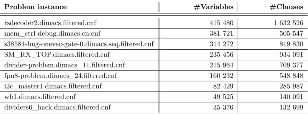
In the experiment we runWalkSATwith the noise-setp= [0.0,0.1,0.2,0.3,0.4,0.5,0.6,0.7,0.8,0.9,1.0], and MAX_FLIPS is set to 300 000 000. We use problem instances listed in table 5.1.

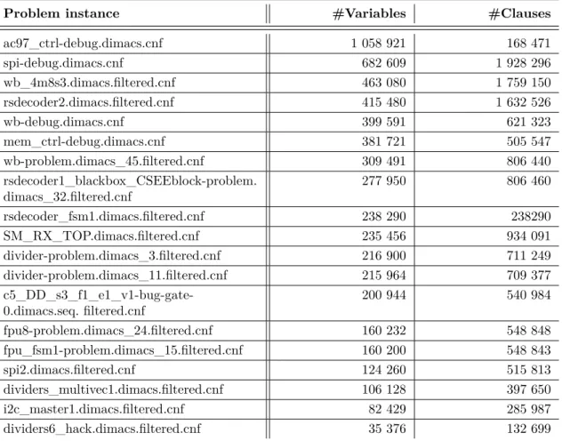
Problem instance #Variables #Clauses

rsdecoder2.dimacs.filtered.cnf 415 480 1 632 526 mem_ctrl-debug.dimacs.cn.cnf 381 721 505 547 s38584-bug-onevec-gate-0.dimacs.seq.filtered.cnf 314 272 819 830 SM_RX_TOP.dimacs.filtered.cnf 235 456 934 091 divider-problem.dimacs_11.filtered.cnf 215 964 709 377 fpu8-problem.dimacs_24.filtered.cnf 160 232 548 848 i2c_master1.dimacs.filtered.cnf 82 429 285 987 wb1.dimacs.filtered.cnf 49 525 140 091 dividers6_hack.dimacs.filtered.cnf 35 376 132 699

Table 5.1: Problem instances used in the experiments, 9 in total. Listed with number of variables and clauses.

5.4.1

Results

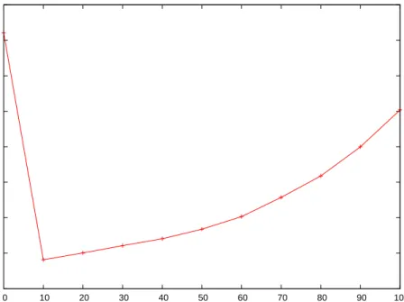
Figure 5.1 shows a noise graph for the problem fpu8-problem.dimacs_24.filtered.cnf. We observe that a bigger noise value increases the number of unsatisfied clauses.

3000 4000 5000 6000 7000 8000 9000 10000 11000 12000 0 10 20 30 40 50 60 70 80 90 100 #Unsatisfied Clauses Noise (%)

Figure 5.1: Problem instance fpu8-problem.dimacs_24.filtered.cnf, |variables| =160 232, |clauses| = 548 848. Vertical axis gives the number of unsatisfied clauses, horizontal axis represents the noise p.

(31)

CHAPTER 5. WALKSAT

The figure below shows WalkSAT solving wb1.dimacs.filtered.cnf. We observe that p= 10% is a good value for the noise parameter.

400 600 800 1000 1200 1400 1600 0 10 20 30 40 50 60 70 80 90 100 #Unsatisfied Clauses Noise (%)

Figure 5.2: Problem instance wb1.dimacs.filtered.cnf, |variables| = 49 525, |clauses| = 140 091. Vertical

axis gives the number of unsatisfied clauses, horizontal axis represents the noisep.

1000 2000 3000 4000 5000 6000 7000 8000 9000 0 10 20 30 40 50 60 70 80 90 100 #Unsatisfied Clauses Noise (%)

Figure 5.3: Problem instance 38584-bug-onevec-gate-0.dimacs.seq.filtered.cnf, |variables| = 314 272,

|clauses| = 819 830. Vertical axis gives the number of unsatisfied clauses, horizontal axis

rep-resents the noisep.

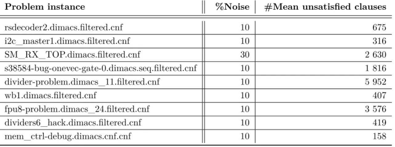
We see that the number of unsatisfied clauses in figures 5.2 and 5.3 is very high at 0% noise, and the same for 100%. The optimal noise seems to be 10% for these two as well. Remaining results are given in table 5.2 below, with optimal noise and number of unsatisfied clauses for each problem.

(32)

CHAPTER 5. WALKSAT

Problem instance %Noise #Mean unsatisfied clauses rsdecoder2.dimacs.filtered.cnf 10 675 i2c_master1.dimacs.filtered.cnf 10 316 SM_RX_TOP.dimacs.filtered.cnf 30 2 630 s38584-bug-onevec-gate-0.dimacs.seq.filtered.cnf 10 1 816 divider-problem.dimacs_11.filtered.cnf 10 5 952 wb1.dimacs.filtered.cnf 10 407 fpu8-problem.dimacs_24.filtered.cnf 10 3 576 dividers6_hack.dimacs.filtered.cnf 10 419 mem_ctrl-debug.dimacs.cnf.cnf 10 158

Table 5.2: Industrial problem instances with the optimal noise for WalkSAT.

The results suggest that WalkSAT prefers 10% noise on most of the industrial problems shown in table 5.2. The results also indicate that WalkSATneeds a rather fair amount of greedy moves compared to random moves when solving industrial MAXSAT problems. Based on this we conclude thatp= 10% is the optimal noise for these problems.

(33)

Chapter 6

Combining WalkSAT with

Multilevel Techniques

In this chapter we extend WalkSAT with multilevel techniques. We start with an introduction of the multilevel paradigm in section 6.1. How this paradigm can be applied in a MAXSAT context is given in section 6.2. In section 6.3 we present our solution where we extendWalkSATwith multilevel techniques. Section 6.4 ends this chapter with benchmarking and corresponding results.

6.1

Introduction to multilevel techniques

We give an informal introduction to the multilevel paradigm by the following everyday example: Imagine you have bought a new house and you are in the process of moving your belongings from your old apartment to your new house. There are several ways to do this. It is possible to think of this as an optimization problem, where the goal is to avoid unnecessary back-and-forth trips between your old and new home. Let us say we have a large amount of objects in different shapes and sizes that we want to move. Obviously, moving these objects one-by-one would not be very efficient. If we had chosen this method, we would have spent a lot of time and trips. However, if we packed several objects into one box, we would be able to move more objects at the same time. Basically what we do is to gather, or cluster, several objects into one object, see figure 6.1. We have gone from one big problem, many single objects, to a smaller problem where the single objects can be seen as one object. Our problem now consists of one box that encapsulates several objects. Hopefully, it now becomes more efficient and easier to move your belongings to your new house.

multilevel techniques

1 object 5 objects

Figure 6.1: Clustering single objects. Single objects can be seen as one object when clustered.

With the example above in mind, there exists several problems where multilevel techniques can and have been applied. Multilevel techniques have been utilized in Graph Coloring [37] and on the well-known combinatorial optimization problem called The Travelling Salesman Problem (TSP) [38,39]. In the next section we explain how the multilevel paradigm can be applied to solve MAXSAT problems.

(34)

CHAPTER 6. COMBINING WALKSAT WITH MULTILEVEL TECHNIQUES

6.2

Multilevel techniques in a MAXSAT context

In chapter 3 we briefly reviewed Bouhmala’s work on solving the SAT problem with multilevel techniques. We will now go into more details, and explain multilevel techniques in a SAT context. Due to the similarities between SAT and MAXSAT, we assume the reader acknowledges that this technique is applicable to MAXSAT in an identical way.

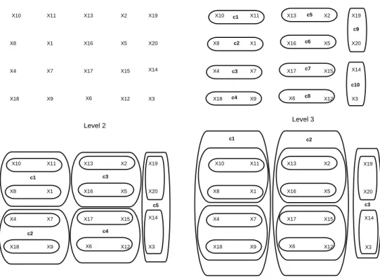
The multilevel algorithm, or paradigm, consists of 4 steps or phases: (1) reduction, (2) initial solution, (3) projection, and (4) refinement. The idea is that the SAT problem can be split up into smaller problems, i.e. multiple levels starting from the start state (level 0) to a given maximum reduced state (level N). Each level is simpler than the previous level. An illustration of the reduction phase is given in figure 6.2.

X3 X6 X5 X1 X4 X7 X9 X8 X2 X10 X11 X12 X13 X14 X15 X16 X17 X18 X20 Level 0 X19 Level 1 X3 X6 X5 X1 X4 X7 X9 X8 X2 X10 X11 X12 X13 X14 X15 X16 X17 X18 X20 X19 X3 X6 X5 X1 X4 X7 X9 X8 X2 X10 X11 X12 X13 X14 X15 X16 X17 X18 X20 X19 X3 X6 X5 X1 X4 X7 X9 X8 X2 X10 X11 X12 X13 X14 X15 X16 X17 X18 X20 X19 Level 2 Level 3 c1 c2 c3 c1 c2 c3 c4 c5 c1 c2 c3 c4 c5 c6 c7 c8 c9 c10

Figure 6.2: Clustering and reduction of variables. |Variables| = 20, |variables per cluster| = 2, |levels| = 3

(not counting level 0).X denotes a variable, andcdenotes a cluster.

The first step, or the reduction process, combines two variables at random1from level 0 (also called

the top level in multilevel terminology) into a cluster, and continues doing the same operation

until there are no more variables to combine. All the clusters that have been made, are said to be contained in level 1. This means one such reduction step, takes us from level X to level X+1. Be aware that below level 0, instead of combining variables, the process would combine clusters since there are no more variables. Note that if there is only one variable or cluster left after all the other variables or clusters have been combined, then this variable or cluster is copied to the next level. An example of this can be seen in figure 6.2; clusterc5 in level 2 is copied to level 3 as clusterc3. In algorithm 4 below (an algorithm from [8] and slightly modified) we can see that reduction continues until the desired amount of levels has been created. In multilevel terminology we call the final level either the lowest level, bottom level or level N. As is evident from the illustration in figure 6.2 we see that level N corresponds to level 3. We also see that there are 20 variables in level 0, and in level 1 two and two of these variables areclustered together. Then at level 2, we have clusters of two and two clusters from level 1. Finally in level 3 we have clusters of two and two clusters from level 2.

1

Note that due to illustrational purposes, figure 6.2 contains clusters with variables combined in an orderly fashion.

(35)

CHAPTER 6. COMBINING WALKSAT WITH MULTILEVEL TECHNIQUES

When we have finished reducing the problem according to some level limit (e.g. maximum of 3 levels) then we are left with level N. We now choose to assign an initial solution to each of the clusters in level N. In a SAT or MAXSAT context, this initial solution is a cluster assignment of truth values. Looking at the illustration in figure 6.2 this corresponds to setting each clus-ter in level 3 to either T RU E or F ALSE. An example of such a cluster assignment would be

c1=T RU E, c2=T RU E, c3=F ALSE. Note that we can either think of a cluster as a single vari-able, or as a collection of variables. If we think of the clusters as collections of variables, we say that if a cluster is assigned a truth value then all subclusters and hence all subvariables are assigned that same truth value.

Algorithm 4

The multilevel paradigm

1:

{

Input:

SAT problem

P

0

}

2:

{

Output:

Solution

S

f inal(P0)

}

3: