Dryad: Distributed Data-Parallel Programs from Sequential Building Blocks

(1)

Dryad: Distributed Data-Parallel Programs from Sequential

Building Blocks

Michael Isard

Microsoft Research, Silicon Valley

Mihai Budiu

Yuan Yu

Andrew Birrell

Dennis Fetterly

ABSTRACT

Dryad is a general-purpose distributed execution engine for coarse-grain data-parallel applications. A Dryad applica-tion combines computaapplica-tional “vertices” with communica-tion “channels” to form a dataﬂow graph. Dryad runs the application by executing the vertices of this graph on a set of available computers, communicating as appropriate through ﬁles, TCP pipes, and shared-memory FIFOs.

The vertices provided by the application developer are quite simple and are usually written as sequential programs with no thread creation or locking. Concurrency arises from Dryad scheduling vertices to run simultaneously on multi-ple computers, or on multimulti-ple CPU cores within a computer. The application can discover the size and placement of data at run time, and modify the graph as the computation pro-gresses to make eﬃcient use of the available resources.

Dryad is designed to scale from powerful multi-core sin-gle computers, through small clusters of computers, to data centers with thousands of computers. The Dryad execution engine handles all the diﬃcult problems of creating a large distributed, concurrent application: scheduling the use of computers and their CPUs, recovering from communication or computer failures, and transporting data between ver-tices.

Categories and Subject Descriptors

D.1.3 [PROGRAMMING TECHNIQUES]: Concurrent Programming—Distributed programming

General Terms

Performance, Design, Reliability

Keywords

Concurrency, Distributed Programming, Dataﬂow, Cluster Computing

Permission to make digital or hard copies of all or part of this work for personal or classroom use is granted without fee provided that copies are not made or distributed for profit or commercial advantage and that copies bear this notice and the full citation on the first page. To copy otherwise, to republish, to post on servers or to redistribute to lists, requires prior specific permission and/or a fee.

1.

INTRODUCTION

The Dryad project addresses a long-standing problem: how can we make it easier for developers to write eﬃcient parallel and distributed applications? We are motivated both by the emergence of large-scale internet services that depend on clusters of hundreds or thousands of general-purpose servers, and also by the prediction that future ad-vances in local computing power will come from increas-ing the number of cores on a chip rather than improvincreas-ing the speed or instruction-level parallelism of a single core [3]. Both of these scenarios involve resources that are in a single administrative domain, connected using a known, high-performance communication topology, under central-ized management and control. In such cases many of the hard problems that arise in wide-area distributed systems may be sidestepped: these include high-latency and unre-liable networks, control of resources by separate federated or competing entities, and issues of identity for authentica-tion and access control. Our primary focus is instead on the simplicity of the programming model and the reliability, eﬃciency and scalability of the applications.

For many resource-intensive applications, the simplest way to achieve scalable performance is to exploit data paral-lelism. There has historically been a great deal of work in the parallel computing community both on systems that automatically discover and exploit parallelism in sequential programs, and on those that require the developer to explic-itly expose the data dependencies of a computation. There are still limitations to the power of fully-automatic paral-lelization, and so we build mainly on ideas from the latter research tradition. Condor [37] was an early example of such a system in a distributed setting, and we take more direct inspiration from three other models: shader languages devel-oped for graphic processing units (GPUs) [30, 36], Google’s MapReduce system [16], and parallel databases [18]. In all these programming paradigms, the system dictates a com-munication graph, but makes it simple for the developer to supply subroutines to be executed at speciﬁed graph ver-tices. All three have demonstrated great success, in that large numbers of developers have been able to write con-current software that is reliably executed in a distributed fashion.

We believe that a major reason for the success of GPU shader languages, MapReduce and parallel databases is that the developer is explicitly forced to consider the data paral-lelism of the computation. Once an application is cast into this framework, the system is automatically able to provide the necessary scheduling and distribution. The developer

(2)

need have no understanding of standard concurrency mech-anisms such as threads and fine-grain concurrency control, which are known to be difficult to program correctly. In-stead the system runtime abstracts these issues from the developer, and also deals with many of the hardest dis-tributed computing problems, most notably resource alloca-tion, scheduling, and the transient or permanent failure of a subset of components in the system. By fixing the boundary between the communication graph and the subroutines that inhabit its vertices, the model guides the developer towards an appropriate level of granularity. The system need not try too hard to extract parallelismwithin a developer-provided subroutine, while it can exploit the fact that dependencies are all explicitly encoded in the flow graph to efficiently distribute the executionacross those subroutines. Finally, developers now work at a suitable level of abstraction for writing scalable applications since the resources available at execution time are not generally known at the time the code is written.

The aforementioned systems restrict an application’s com-munication flow for different reasons. GPU shader languages are strongly tied to an efficient underlying hardware imple-mentation that has been tuned to give good performance for common graphics memory-access patterns. MapReduce was designed to be accessible to the widest possible class of developers, and therefore aims for simplicity at the expense of generality and performance. Parallel databases were de-signed for relational algebra manipulations (e.g. SQL) where the communication graph is implicit.

By contrast, the Dryad system allows the developer fine control over the communication graph as well as the subrou-tines that live at its vertices. A Dryad application developer can specify an arbitrary directed acyclic graph to describe the application’s communication patterns, and express the data transport mechanisms (files, TCP pipes, and shared-memory FIFOs) between the computation vertices. This direct specification of the graph also gives the developer greater flexibility to easily compose basic common opera-tions, leading to a distributed analogue of “piping” together traditional Unix utilities such asgrep,sortandhead.

Dryad is notable for allowing graph vertices (and compu-tations in general) to use an arbitrary number of inputs and outputs. MapReduce restricts all computations to take a single input set and generate a single output set. SQL and shader languages allow multiple inputs but generate a single output from the user’s perspective, though SQL query plans internally use multiple-output vertices.

In this paper, we demonstrate that careful choices in graph construction and refinement can substantially improve ap-plication performance, while compromising little on the pro-grammability of the system. Nevertheless, Dryad is cer-tainly a lower-level programming model than SQL or Di-rectX. In order to get the best performance from a native Dryad application, the developer must understand the struc-ture of the computation and the organization and properties of the system resources. Dryad was however designed to be a suitable infrastructure on which to layer simpler, higher-level programming models. It has already been used, by our-selves and others, as a platform for several domain-specific systems that are briefly sketched in Section 7. These rely on Dryad to manage the complexities of distribution, schedul-ing, and fault-tolerance, but hide many of the details of the underlying system from the application developer. They

use heuristics to automatically select and tune appropriate Dryad features, and thereby get good performance for most simple applications.

We summarize Dryad’s contributions as follows:

• We built a general-purpose, high performance distrib-uted execution engine. The Dryad execution engine handles many of the difficult problems of creating a large distributed, concurrent application: scheduling across resources, optimizing the level of concurrency within a computer, recovering from communication or computer failures, and delivering data to where it is needed. Dryad supports multiple different data trans-port mechanisms between computation vertices and explicit dataflow graph construction and refinement. • We demonstrated the excellent performance of Dryad

from a single multi-core computer up to clusters con-sisting of thousands of computers on several nontrivial, real examples. We further demonstrated that Dryad’s fine control over an application’s dataflow graph gives the programmer the necessary tools to optimize trade-offs between parallelism and data distribution over-head. This validated Dryad’s design choices.

• We explored the programmability of Dryad on two fronts. First, we have designed a simple graph descrip-tion language that empowers the developer with ex-plicit graph construction and refinement to fully take advantage of the rich features of the Dryad execution engine. Our user experiences lead us to believe that, while it requires some effort to learn, a programmer can master the APIs required for most of the appli-cations in a couple of weeks. Second, we (and oth-ers within Microsoft) have built simpler, higher-level programming abstractions for specific application do-mains on top of Dryad. This has significantly lowered the barrier to entry and increased the acceptance of Dryad among domain experts who are interested in using Dryad for rapid application prototyping. This further validated Dryad’s design choices.

The next three sections describe the abstract form of a Dryad application and outline the steps involved in writ-ing one. The Dryad scheduler is described in Section 5; it handles all of the work of deciding which physical resources to schedule work on, routing data between computations, and automatically reacting to computer and network fail-ures. Section 6 reports on our experimental evaluation of the system, showing its ﬂexibility and scaling characteris-tics in a small cluster of 10 computers, as well as details of larger-scale experiments performed on clusters with thou-sands of computers. We conclude in Sections 8 and 9 with a discussion of the related literature and of future research directions.

2.

SYSTEM OVERVIEW

The overall structure of a Dryad job is determined by its communication ﬂow. A job is a directed acyclic graph where each vertex is a program and edges represent data channels. It is a logical computation graph that is automat-ically mapped onto physical resources by the runtime. In particular, there may be many more vertices in the graph than execution cores in the computing cluster.

(3)

At run time each channel is used to transport a finite se-quence of structured items. This channel abstraction has several concrete implementations that use shared memory, TCP pipes, or files temporarily persisted in a file system. As far as the program in each vertex is concerned, channels produce and consume heap objects that inherit from a base type. This means that a vertex program reads and writes its data in the same way regardless of whether a channel seri-alizes its data to buffers on a disk or TCP stream, or passes object pointers directly via shared memory. The Dryad sys-tem does not include any native data model for serializa-tion and the concrete type of an item is left entirely up to applications, which can supply their own serialization and deserialization routines. This decision allows us to support applications that operate directly on existing data includ-ing exported SQL tables and textual log files. In practice most applications use one of a small set of library item types that we supply such as newline-terminated text strings and tuples of base types.

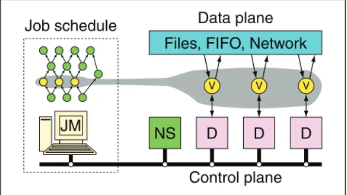
A schematic of the Dryad system organization is shown in Figure 1. A Dryad job is coordinated by a process called the “job manager” (denoted JM in the ﬁgure) that runs either within the cluster or on a user’s workstation with network access to the cluster. The job manager contains the application-speciﬁc code to construct the job’s commu-nication graph along with library code to schedule the work across the available resources. All data is sent directly be-tween vertices and thus the job manager is only responsible for control decisions and is not a bottleneck for any data transfers.

Files, FIFO, Network

Job schedule

Data plane

Control plane

D

NS

V V V

JM

Figure 1: The Dryad system organization.The job manager (JM) consults the name server (NS) to discover the list of available com-puters. It maintains the job graph and schedules running vertices (V) as computers become available using the daemon (D) as a proxy. Vertices exchange data through files, TCP pipes, or shared-memory channels. The shaded bar indicates the vertices in the job that are currently running.

The cluster has a name server (NS) that can be used to enumerate all the available computers. The name server also exposes the position of each computer within the net-work topology so that scheduling decisions can take account of locality. There is a simple daemon (D) running on each computer in the cluster that is responsible for creating pro-cesses on behalf of the job manager. The ﬁrst time a vertex (V) is executed on a computer its binary is sent from the job manager to the daemon and subsequently it is executed from a cache. The daemon acts as a proxy so that the job man-ager can communicate with the remote vertices and monitor the state of the computation and how much data has been

read and written on its channels. It is straightforward to run a name server and a set of daemons on a user workstation to simulate a cluster and thus run an entire job locally while debugging.

A simple task scheduler is used to queue batch jobs. We use a distributed storage system, not described here, that shares with the Google File System [21] the property that large ﬁles can be broken into small pieces that are replicated and distributed across the local disks of the cluster comput-ers. Dryad also supports the use of NTFS for accessing ﬁles directly on local computers, which can be convenient for small clusters with low management overhead.

2.1

An example SQL query

In this section, we describe a concrete example of a Dryad application that will be further developed throughout the re-mainder of the paper. The task we have chosen is representa-tive of a new class of eScience applications, where scientiﬁc investigation is performed by processing large amounts of data available in digital form [24]. The database that we use is derived from the Sloan Digital Sky Survey (SDSS), available online athttp://skyserver.sdss.org.

We chose the most time consuming query (Q18) from a published study based on this database [23]. The task is to identify a “gravitational lens” eﬀect: it ﬁnds all the objects in the database that have neighboring objects within 30 arc seconds such that at least one of the neighbors has a color similar to the primary object’s color. The query can be expressed in SQL as:

select distinct p.objID from photoObjAll p

join neighbors n — call this join “X” on p.objID = n.objID

and n.objID < n.neighborObjID and p.mode = 1

join photoObjAll l — call this join “Y” on l.objid = n.neighborObjID and l.mode = 1 and abs((p.u-p.g)-(l.u-l.g))<0.05 and abs((p.g-p.r)-(l.g-l.r))<0.05 and abs((p.r-p.i)-(l.r-l.i))<0.05 and abs((p.i-p.z)-(l.i-l.z))<0.05

There are two tables involved. The ﬁrst, photoObjAll

has 354,254,163 records, one for each identified astronomical object, keyed by a unique identifierobjID. These records also include the object’s color, as a magnitude (logarithmic brightness) in five bands: u,g,r,iandz. The second table,

neighbors has 2,803,165,372 records, one for each object located within 30 arc seconds of another object. Themode

predicates in the query select only “primary” objects. The

<predicate eliminates duplication caused by theneighbors

relationship being symmetric. The output of joins “X” and “Y” are 932,820,679 and 83,798 records respectively, and the ﬁnal hash emits 83,050 records.

The query uses only a few columns from the tables (the completephotoObjAlltable contains 2 KBytes per record). When executed by SQLServer the query uses an index on

photoObjAllkeyed byobjIDwith additional columns for

mode,u,g,r,iandz, and an index onneighborskeyed by

objIDwith an additionalneighborObjID column. SQL-Server reads just these indexes, leaving the remainder of the tables’ data resting quietly on disk. (In our experimental setup we in fact omitted unused columns from the table, to avoid transporting the entire multi-terabyte database across

(4)

the country.) For the equivalent Dryad computation we ex-tracted these indexes into two binary files, “ugriz.bin” and “neighbors.bin,” each sorted in the same order as the in-dexes. The “ugriz.bin” file has 36-byte records, totaling 11.8 GBytes; “neighbors.bin” has 16-byte records, total-ing 41.8 GBytes. The output of join “X” totals 31.3 GBytes, the output of join “Y” is 655 KBytes and the final output is 649 KBytes. D D M M 4n S S 4n Y Y U U U N U N H n n X n X

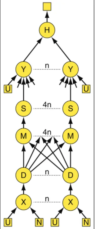
Figure 2: The communica-tion graph for an SQL query.

Details are in Section 2.1. We mapped the query to

the Dryad computation shown in Figure 2. Both data ﬁles are partitioned inton approx-imately equal parts (that we call U1 through Un and N1 throughNn) byobjIDranges, and we use custom C++ item objects for each data record in the graph. The vertices

Xi (for 1 ≤ i ≤ n) imple-ment join “X” by taking their partitioned Ui and Ni inputs and merging them (keyed on

objID and ﬁltered by the

<expression andp.mode=1) to produce records containing

objID,neighborObjID, and the color columns correspond-ing toobjID. The D vertices distribute their output records to the M vertices, partition-ing byneighborObjIDusing a range partitioning function four times ﬁner than that used for the input ﬁles. The number four was chosen so that four pipelines will execute in paral-lel on each computer, because our computers have four

pro-cessors each. The M vertices perform a non-deterministic merge of their inputs and the S vertices sort on neigh-borObjID using an in-memory Quicksort. The output records fromS4i−3. . . S4i (fori= 1 throughn) are fed into

Yi where they are merged with another read of Ui to im-plement join “Y”. This join is keyed onobjID(fromU) =

neighborObjID(fromS), and is ﬁltered by the remainder of the predicate, thus matching the colors. The outputs of theY vertices are merged into a hash table at theH vertex to implement thedistinctkeyword in the query. Finally, an enumeration of this hash table delivers the result. Later in the paper we include more details about the implementation of this Dryad program.

3.

DESCRIBING A DRYAD GRAPH

We have designed a simple language that makes it easy to specify commonly-occurring communication idioms. It is currently “embedded” for convenience in C++ as a library using a mixture of method calls and operator overloading.

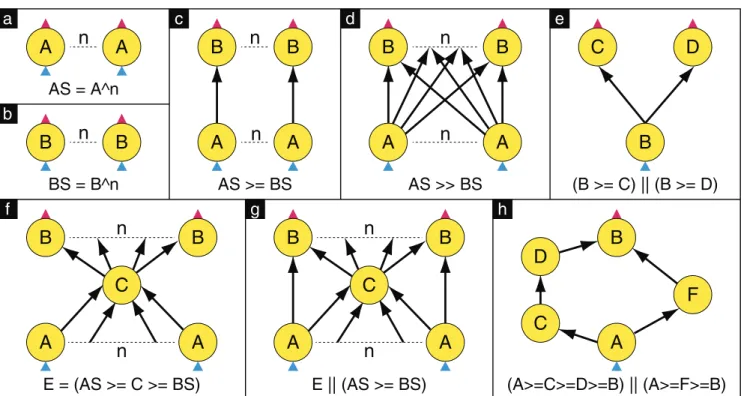
Graphs are constructed by combining simpler subgraphs using a small set of operations shown in Figure 3. All of the operations preserve the property that the resulting graph is acyclic. The basic object in the language is a graph:

G=VG, EG, IG, OG.

Gcontains a sequence of verticesVG, a set of directed edges

EG, and two setsIG⊆VGand OG ⊆VGthat “tag” some of the vertices as beinginputs andoutputs respectively. No graph can contain a directed edge entering an input vertex inIG, nor one leaving an output vertex inOG, and these tags are used below in composition operations. The input and output edges of a vertex are ordered so an edge connects speciﬁc “ports” on a pair of vertices, and a given pair of vertices may be connected by multiple edges.

3.1

Creating new vertices

The Dryad libraries deﬁne a C++ base class from which all vertex programs inherit. Each such program has a tex-tual name (which is unique within an application) and a static “factory” that knows how to construct it. A graph vertex is created by calling the appropriate static program factory. Any required vertex-speciﬁc parameters can be set at this point by calling methods on the program object. These parameters are then marshaled along with the unique vertex name to form a simple closure that can be sent to a remote process for execution.

A singleton graph is generated from a vertex v as G = (v),∅,{v},{v}. A graph can be cloned into a new graph containing k copies of its structure using the ^ operator whereC = G^kis deﬁned as:

C=VG1⊕ · · · ⊕VGk, EG1 ∪ · · · ∪EGk,

IG1 ∪ · · · ∪IGk, OG1 ∪ · · · ∪OkG.

Here Gn =VGn, EGn, IGn, OGn is a “clone” of G containing copies of all ofG’s vertices and edges,⊕denotes sequence concatenation, and each cloned vertex inherits the type and parameters of its corresponding vertex inG.

3.2

Adding graph edges

New edges are created by applying a composition opera-tion to two existing graphs. There is a family of composi-tions all sharing the same basic structure: C = A ◦ Bcreates a new graph:

C=VA⊕VB, EA∪EB∪Enew, IA, OB

where Ccontains the union of all the vertices and edges in

A and B, with A’s inputs and B’s outputs. In addition, directed edgesEnew are introduced between vertices inOA andIB. VAandVB are enforced to be disjoint at run time, and sinceAandB are both acyclic,C is also.

Compositions diﬀer in the set of edgesEnewthat they add into the graph. We deﬁne two standard compositions:

• A >= Bforms a pointwise composition as shown in Fig-ure 3(c). If |OA| ≥ |IB|then a single outgoing edge is created from each of A’s outputs. The edges are assigned in round-robin to B’s inputs. Some of the vertices inIB may end up with more than one incom-ing edge. If |IB| > |OA|, a single incoming edge is created to each ofB’s inputs, assigned in round-robin fromA’s outputs.

• A >> B forms the complete bipartite graph between

OA andIB and is shown in Figure 3(d).

We allow the user to extend the language by implementing new composition operations.

(5)

AS = A^n

n

A

BS = B^n

n

B

E = (AS >= C >= BS)

n

C

A

B

E || (AS >= BS)

n

C

A

B

(A>=C>=D>=B) || (A>=F>=B)

D

C

F

A

B

A

B

AS >> BS

n

B

C

D

(B >= C) || (B >= D)

AS >= BS

A

n

B

n

a

c

d

e

f

g

h

b

Figure 3: The operators of the graph description language.Circles are vertices and arrows are graph edges. A triangle at the bottom of a vertex indicates aninputand one at the top indicates anoutput. Boxes (a) and (b) demonstrate cloning individual vertices using the^operator. The two standard connection operations are pointwise composition using>=shown in (c) and complete bipartite composition using>>shown in (d). (e) illustrates a merge using||. The second line of the figure shows more complex patterns. The merge in (g) makes use of a “subroutine” from (f) and demonstrates a bypass operation. For example, each A vertex might output a summary of its input to C which aggregates them and forwards the global statistics to every B. Together the B vertices can then distribute the original dataset (received from A) into balanced partitions. An asymmetric fork/join is shown in (h).

3.3

Merging two graphs

The ﬁnal operation in the language is||, which merges two graphs. C = A || Bcreates a new graph:

C=VA⊕∗VB, EA∪EB, IA∪∗IB, OA∪∗OB where, in contrast to the composition operations, it is not required that A and B be disjoint. VA⊕∗VB is the con-catenation ofVA andVB with duplicates removed from the second sequence. IA∪∗IBmeans the union ofAandB’s in-puts, minus any vertex that has an incoming edge following the merge (and similarly for the output case). If a vertex is contained inVA∩VB its input and output edges are con-catenated so that the edges in EA occur ﬁrst (with lower port numbers). This simpliﬁcation forbids certain graphs with “crossover” edges, however we have not found this re-striction to be a problem in practice. The invariant that the merged graph be acyclic is enforced by a run-time check.

The merge operation is extremely powerful and makes it easy to construct typical patterns of communication such as fork/join and bypass as shown in Figures 3(f)–(h). It also provides the mechanism for assembling a graph “by hand” from a collection of vertices and edges. So for example, a tree with four verticesa, b, c, anddmight be constructed asG = (a>=b) || (b>=c) || (b>=d).

The graph builder program to construct the query graph in Figure 2 is shown in Figure 4.

3.4

Channel types

By default each channel is implemented using a tempo-rary ﬁle: the producer writes to disk (typically on its local computer) and the consumer reads from that ﬁle.

In many cases multiple vertices will ﬁt within the re-sources of a single computer so it makes sense to execute them all within the same process. The graph language has an “encapsulation” command that takes a graphGand re-turns a new vertex vG. When vG is run as a vertex pro-gram, the job manager passes it a serialization of G as an invocation parameter, and it runs all the vertices of G si-multaneously within the same process, connected by edges implemented using shared-memory FIFOs. While it would always be possible to write a custom vertex program with the same semantics asG, allowing encapsulation makes it ef-ﬁcient to combine simple library vertices at the graph layer rather than re-implementing their functionality as a new vertex program.

Sometimes it is desirable to place two vertices in the same process even though they cannot be collapsed into a single graph vertex from the perspective of the scheduler. For ex-ample, in Figure 2 the performance can be improved by placing the ﬁrst D vertex in the same process as the ﬁrst four M and S vertices and thus avoiding some disk I/O, however theS vertices cannot be started until all of theD

vertices complete.

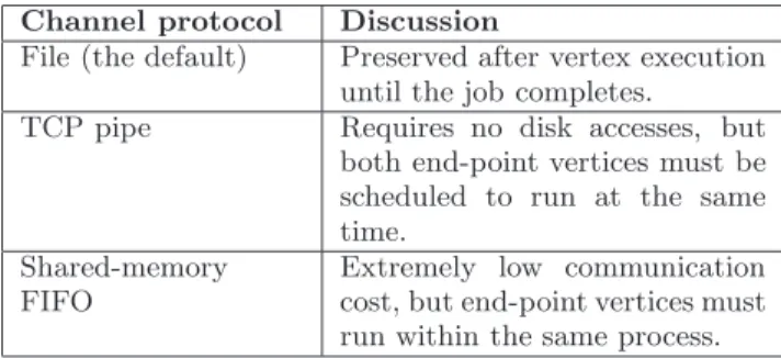
When creating a set of graph edges, the user can option-ally specify the transport protocol to be used. The available protocols are listed in Table 1. Vertices that are connected using shared-memory channels are executed within a single process, though they are individually started as their inputs become available and individually report completion.

Because the dataﬂow graph is acyclic, scheduling dead-lock is impossible when all channels are either written to temporary ﬁles or use shared-memory FIFOs hidden within

(6)

GraphBuilder XSet = moduleX^N; GraphBuilder DSet = moduleD^N; GraphBuilder MSet = moduleM^(N*4); GraphBuilder SSet = moduleS^(N*4); GraphBuilder YSet = moduleY^N; GraphBuilder HSet = moduleH^1;

GraphBuilder XInputs = (ugriz1 >= XSet) || (neighbor >= XSet); GraphBuilder YInputs = ugriz2 >= YSet;

GraphBuilder XToY = XSet >= DSet >> MSet >= SSet; for (i = 0; i < N*4; ++i)

{

XToY = XToY || (SSet.GetVertex(i) >= YSet.GetVertex(i/4));

}

GraphBuilder YToH = YSet >= HSet; GraphBuilder HOutputs = HSet >= output;

GraphBuilder final = XInputs || YInputs || XToY || YToH || HOutputs;

Figure 4: An example graph builder program.The communication graph generated by this program is shown in Figure 2.

Channel protocol Discussion

File (the default) Preserved after vertex execution until the job completes.

TCP pipe Requires no disk accesses, but both end-point vertices must be scheduled to run at the same time.

Shared-memory FIFO

Extremely low communication cost, but end-point vertices must run within the same process.

Table 1: Channel types.

encapsulated acyclic subgraphs. However, allowing the de-veloper to use pipes and “visible” FIFOs can cause dead-locks. Any connected component of vertices communicating using pipes or FIFOs must all be scheduled in processes that are concurrently executing, but this becomes impossible if the system runs out of available computers in the cluster.

This breaks the abstraction that the user need not know the physical resources of the system when writing the appli-cation. We believe that it is a worthwhile trade-off, since, as reported in our experiments in Section 6, the resulting per-formance gains can be substantial. Note also that the sys-tem could always avoid deadlock by “downgrading” a pipe channel to a temporary file, at the expense of introducing an unexpected performance cliff.

3.5

Job inputs and outputs

Large input ﬁles are typically partitioned and distributed across the computers of the cluster. It is therefore natural to group a logical input into a graphG=VP,∅,∅, VPwhere

VP is a sequence of “virtual” vertices corresponding to the partitions of the input. Similarly on job completion a set of output partitions can be logically concatenated to form a single named distributed ﬁle. An application will generally interrogate its input graphs to read the number of partitions at run time and automatically generate the appropriately replicated graph.

3.6

Job Stages

When the graph is constructed every vertex is placed in a “stage” to simplify job management. The stage topology can be seen as a “skeleton” or summary of the overall job,

and the stage topology of our example Skyserver query ap-plication is shown in Figure 5. Each distinct type of vertex is grouped into a separate stage. Most stages are connected using the>=operator, whileDis connected toM using the

>>operator. The skeleton is used as a guide for generating summaries when monitoring a job, and can also be exploited by the automatic optimizations described in Section 5.2.

4.

WRITING A VERTEX PROGRAM

D

M

S

Y

U

N

H

X

Figure 5: The stages of the Dryad compu-tation from Figure 2.

Section 3.6 has details. The primary APIs for writing a

Dryad vertex program are exposed through C++ base classes and ob-jects. It was a design requirement for Dryad vertices to be able to incor-porate legacy source and libraries, so we deliberately avoided adopting any Dryad-specific language or sandbox-ing restrictions. Most of the existsandbox-ing code that we anticipate integrating into vertices is written in C++, but it is straightforward to implement API wrappers so that developers can write vertices in other languages, for example C#. There is also significant value for some domains in being able to run unmodified legacy executables in vertices, and so we support this as explained in Section 4.2 below.

4.1

Vertex execution

Dryad includes a runtime library that is responsible for setting up and executing vertices as part of a dis-tributed computation. As outlined in Section 3.1 the runtime receives a clo-sure from the job manager describing the vertex to be run, and URIs de-scribing the input and output chan-nels to connect to it. There is cur-rently no type-checking for channels and the vertex must be able to

deter-mine, either statically or from the invocation parameters, the types of the items that it is expected to read and write

(7)

on each channel in order to supply the correct serialization routines. The body of a vertex is invoked via a standard

Main method that includes channel readers and writers in its argument list. The readers and writers have a blocking interface to read or write the next item, which suﬃces for most simple applications. The vertex can report status and errors to the job manager, and the progress of channels is automatically monitored.

Many developers ﬁnd it convenient to inherit from pre-deﬁned vertex classes that hide the details of the underlying channels and vertices. We supplymap and reduce classes with similar interfaces to those described in [16]. We have also written a variety of others including a general-purpose

distributethat takes a single input stream and writes on multiple outputs, andjoins that call a virtual method with every matching record tuple. These “classes” are simply vertices like any other, so it is straightforward to write new ones to support developers working in a particular domain.

4.2

Legacy executables

We provide a library “process wrapper” vertex that forks an executable supplied as an invocation parameter. The wrapper vertex must work with arbitrary data types, so its “items” are simply fixed-size buffers that are passed unmod-ified to the forked process using named pipes in the file-system. This allows unmodified pre-existing binaries to be run as Dryad vertex programs. It is easy, for example, to invokeperlscripts orgrepat some vertices of a Dryad job.

4.3

Efficient pipelined execution

Most Dryad vertices contain purely sequential code. We also support an event-based programming style, using a shared thread pool. The program and channel interfaces have asynchronous forms, though unsurprisingly it is harder to use the asynchronous interfaces than it is to write se-quential code using the synchronous interfaces. In some cases it may be worth investing this eﬀort, and many of the standard Dryad vertex classes, including non-deterministic merge, sort, and generic maps and joins, are built using the event-based programming style. The runtime automatically distinguishes between vertices which can use a thread pool and those that require a dedicated thread, and therefore en-capsulated graphs which contain hundreds of asynchronous vertices are executed eﬃciently on a shared thread pool.

The channel implementation schedules read, write, seri-alization and deseriseri-alization tasks on a thread pool shared between all channels in a process, and a vertex can concur-rently read or write on hundreds of channels. The runtime tries to ensure eﬃcient pipelined execution while still pre-senting the developer with the simple abstraction of reading and writing a single record at a time. Extensive use is made of batching [28] to try to ensure that threads process hun-dreds or thousands of records at a time without touching a reference count or accessing a shared queue. The exper-iments in Section 6.2 substantiate our claims for the eﬃ-ciency of these abstractions: even single-node Dryad appli-cations have throughput comparable to that of a commercial database system.

5.

JOB EXECUTION

The scheduler inside the job manager keeps track of the state and history of each vertex in the graph. At present if the job manager’s computer fails the job is terminated,

though the vertex scheduler could employ checkpointing or replication to avoid this. A vertex may be executed mul-tiple times over the length of the job due to failures, and more than one instance of a given vertex may be executing at any given time. Each execution of the vertex has a ver-sion number and a corresponding “execution record” that contains the state of that execution and the versions of the predecessor vertices from which its inputs are derived. Each execution names its file-based output channels uniquely us-ing its version number to avoid conflicts among versions. If the entire job completes successfully then each vertex selects a successful execution and renames its output files to their correct final forms.

When all of a vertex’s input channels become ready a new execution record is created for the vertex and placed in a scheduling queue. A disk-based channel is considered to be ready when the entire ﬁle is present. A channel that is a TCP pipe or shared-memory FIFO is ready when the predecessor vertex has at least one running execution record. A vertex and any of its channels may each specify a “hard-constraint” or a “preference” listing the set of computers on which it would like to run. The constraints are combined and attached to the execution record when it is added to the scheduling queue and they allow the application writer to require that a vertex be co-located with a large input ﬁle, and in general let the scheduler preferentially run computa-tions close to their data.

At present the job manager performs greedy scheduling based on the assumption that it is the only job running on the cluster. When an execution record is paired with an available computer the remote daemon is instructed to run the speciﬁed vertex, and during execution the job manager receives periodic status updates from the vertex. If every vertex eventually completes then the job is deemed to have completed successfully. If any vertex is re-run more than a set number of times then the entire job is failed.

Files representing temporary channels are stored in di-rectories managed by the daemon and cleaned up after the job completes, and vertices are killed by the daemon if their “parent” job manager crashes. We have a simple graph visu-alizer suitable for small jobs that shows the state of each ver-tex and the amount of data transmitted along each channel as the computation progresses. A web-based interface shows regularly-updated summary statistics of a running job and can be used to monitor large computations. The statistics include the number of vertices that have completed or been re-executed, the amount of data transferred across channels, and the error codes reported by failed vertices. Links are provided from the summary page that allow a developer to download logs or crash dumps for further debugging, along with a script that allows the vertex to be re-executed in isolation on a local machine.

5.1

Fault tolerance policy

Failures are to be expected during the execution of any distributed application. Our default failure policy is suitable for the common case that all vertex programs are determin-istic.1 Because our communication graph is acyclic, it is relatively straightforward to ensure that every terminating execution of a job with immutable inputs will compute the 1_{The deﬁnition of job completion and the treatment of job} outputs above also implicitly assume deterministic execu-tion.

(8)

same result, regardless of the sequence of computer or disk failures over the course of the execution.

When a vertex execution fails for any reason the job man-ager is informed. If the vertex reported an error cleanly the process forwards it via the daemon before exiting; if the process crashes the daemon notifies the job manager; and if the daemon fails for any reason the job manager receives a heartbeat timeout. If the failure was due to a read error on an input channel (which is be reported cleanly) the default policy also marks the execution record that generated that version of the channel as failed and terminates its process if it is running. This will cause the vertex that created the failed input channel to be re-executed, and will lead in the end to the offending channel being re-created. Though a newly-failed execution record may have non-failed successor records, errors need not be propagated forwards: since ver-tices are deterministic two successors may safely compute using the outputs of different execution versions. Note how-ever that under this policy an entire connected component of vertices connected by pipes or shared-memory FIFOs will fail as a unit since killing a running vertex will cause it to close its pipes, propagating errors in both directions along those edges. Any vertex whose execution record is set to failed is immediately considered for re-execution.

As Section 3.6 explains, each vertex belongs to a “stage,” and each stage has a manager object that receives a callback on every state transition of a vertex execution in that stage, and on a regular timer interrupt. Within this callback the stage manager holds a global lock on the job manager data-structures and can therefore implement quite sophisticated behaviors. For example, the default stage manager includes heuristics to detect vertices that are running slower than their peers and schedule duplicate executions. This prevents a single slow computer from delaying an entire job and is similar to the backup task mechanism reported in [16]. In future we may allow non-deterministic vertices, which would make fault-tolerance more interesting, and so we have imple-mented our policy via an extensible mechanism that allows non-standard applications to customize their behavior.

5.2

Run-time graph refinement

We have used the stage-manager callback mechanism to implement run-time optimization policies that allow us to scale to very large input sets while conserving scarce network bandwidth. Some of the large clusters we have access to have their network provisioned in a two-level hierarchy, with a dedicated mini-switch serving the computers in each rack, and the per-rack switches connected via a single large core switch. Therefore where possible it is valuable to schedule vertices as much as possible to execute on the same computer or within the same rack as their input data.

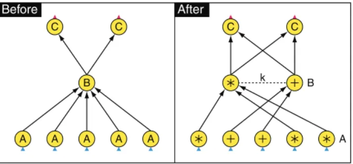
If a computation is associative and commutative, and per-forms a data reduction, then it can benefit from an aggrega-tion tree. As shown in Figure 6, a logical graph connecting a set of inputs to a single downstream vertex can be refined by inserting a new layer of internal vertices, where each internal vertex reads data from a subset of the inputs that are close in network topology, for example on the same computer or within the same rack. If the internal vertices perform a data reduction, the overall network traffic between racks will be reduced by this refinement. A typical application would be a histogramming operation that takes as input a set of partial histograms and outputs their union. The implementation in

A A A A A A B Before After k Z B

Figure 6: A dynamic refinement for aggregation. The logical graph on the left connects every input to the single output. The lo-cations and sizes of the inputs are not known until run time when it is determined which computer each vertex is scheduled on. At this point the inputs are grouped into subsets that are close in network topology, and an internal vertex is inserted for each subset to do a local aggregation, thus saving network bandwidth. The internal ver-tices are all of the same user-supplied type, in this case shown as “Z.” In the diagram on the right, vertices with the same label (’+’ or ’*’) are executed close to each other in network topology.

Dryad simply attaches a custom stage manager to the input layer. As this aggregation manager receives callback notiﬁ-cations that upstream vertices have completed, it rewrites the graph with the appropriate reﬁnements.

The operation in Figure 6 can be performed recursively to generate as many layers of internal vertices as required. We have also found a “partial aggregation” operation to be very useful. This refinement is shown in Figure 7; having grouped the inputs intoksets, the optimizer replicates the downstream vertex k times to allow all of the sets to be processed in parallel. Optionally, the partial refinement can be made to propagate through the graph so that an entire pipeline of vertices will be replicatedktimes (this behavior is not shown in the figure). An example of the application of this technique is described in the experiments in Section 6.3. Since the aggregation manager is notified on the completion of upstream vertices, it has access to the size of the data written by those vertices as well as its location. A typical grouping heuristic ensures that a downstream vertex has no more than a set number of input channels, or a set volume of input data. A special case of partial refinement can be performed at startup to size the initial layer of a graph so that, for example, each vertex processes multiple inputs up to some threshold with the restriction that all the inputs must lie on the same computer.

Because input data can be replicated on multiple com-puters in a cluster, the computer on which a graph vertex is scheduled is in general non-deterministic. Moreover the

A A A A A A

B B

C C C C

Before After

k

Figure 7: A partial aggregation refinement. Following an input grouping as in Figure 6 intoksets, the successor vertex is replicated

(9)

amount of data written in intermediate computation stages is typically not known before a computation begins. There-fore dynamic reﬁnement is often more eﬃcient than attempt-ing a static groupattempt-ing in advance.

Dynamic reﬁnements of this sort emphasize the power of overlaying a physical graph with its “skeleton.” For many applications, there is an equivalence class of graphs with the same skeleton that compute the same result. Varying the number of vertices in each stage, or their connectivity, while preserving the graph topology at the stage level, is merely a (dynamic) performance optimization.

6.

EXPERIMENTAL EVALUATION

Dryad has been used for a wide variety of applications, in-cluding relational queries, large-scale matrix computations, and many text-processing tasks. For this paper we examined the effectiveness of the Dryad system in detail by running two sets of experiments. The first experiment takes the SQL query described in Section 2.1 and implements it as a Dryad application. We compare the Dryad performance with that of a traditional commercial SQL server, and we analyze the Dryad performance as the job is distributed across different numbers of computers. The second is a simple map-reduce style data-mining operation, expressed as a Dryad program and applied to 10.2 TBytes of data using a cluster of around 1800 computers.

The strategies we adopt to build our communication ﬂow graphs are familiar from the parallel database literature [18] and include horizontally partitioning the datasets, exploit-ing pipelined parallelism within processes and applyexploit-ing ex-change operations to communicate partial results between the partitions. None of the application-level code in any of our experiments makes explicit use of concurrency primi-tives.

6.1

Hardware

The SQL query experiments were run on a cluster of 10 computers in our own laboratory, and the data-mining tests were run on a cluster of around 1800 computers embed-ded in a data center. Our laboratory computers each had 2 dual-core Opteron processors running at 2 GHz (i.e., 4 CPUs total), 8 GBytes of DRAM (half attached to each processor chip), and 4 disks. The disks were 400 GByte Western Dig-ital WD40 00YR-01PLB0 SATA drives, connected through a Silicon Image 3114 PCI SATA controller (66MHz, 32-bit). Network connectivity was by 1 Gbit/sec Ethernet links con-necting into a single non-blocking switch. One of our labo-ratory computers was dedicated to running SQLServer and its data was stored in 4 separate 350 GByte NTFS volumes, one on each drive, with SQLServer configured to do its own data striping for the raw data and for its temporary tables. All the other laboratory computers were configured with a single 1.4 TByte NTFS volume on each computer, created by software striping across the 4 drives. The computers in the data center had a variety of configurations, but were typically roughly comparable to our laboratory equipment. All the computers were running Windows Server 2003 En-terprise x64 edition SP1.

6.2

SQL Query

The query for this experiment is described in Section 2.1 and uses the Dryad communication graph shown in Figure 2. SQLServer 2005’s execution plan for this query was very

close to the Dryad computation, except that it used an ex-ternal hash join for “Y” in place of the sort-merge we chose for Dryad. SQLServer takes slightly longer if it is forced by a query hint to use a sort-merge join.

For our experiments, we used two variants of the Dryad graph: “in-memory” and “two-pass.” In both variants com-munication from eachMithrough its correspondingSitoY is by a shared-memory FIFO. This pulls four sorters into the same process to execute in parallel on the four CPUs in each computer. In the “in-memory” variant only, communication from eachDito its four correspondingMjvertices is also by a shared-memory FIFO and the rest of theDi→Mk edges use TCP pipes. All other communication is through NTFS temporary ﬁles in both variants.

There is good spatial locality in the query, which improves as the number of partitions (n) decreases: for n = 40 an average of 80% of the output ofDigoes to its corresponding

Mi, increasing to 88% for n= 6. In either variantnmust be large enough that every sort executed by a vertexSiwill ﬁt into the computer’s 8 GBytes of DRAM (or else it will page). With the current data, this threshold is atn= 6.

Note that the non-deterministic merge in M randomly permutes its output depending on the order of arrival of items on its input channels and this technically violates the requirement that all vertices be deterministic. This does not cause problems for our fault-tolerance model because the sortSi “undoes” this permutation, and since the edge from Mi to Si is a shared-memory FIFO within a single process the two vertices fail (if at all) in tandem and the non-determinism never “escapes.”

The in-memory variant requires at leastncomputers since otherwise theSvertices will deadlock waiting for data from an X vertex. The two-pass variant will run on any num-ber of computers. One way to view this trade-off is that by adding the file buffering in the two-pass variant we in ef-fect converted to using a two-pass external sort. Note that the conversion from the in-memory to the two-pass program simply involves changing two lines in the graph construction code, with no modifications to the vertex programs.

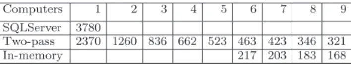
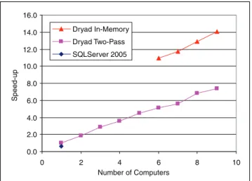
We ran the two-pass variant using n = 40, varying the number of computers from 1 to 9. We ran the in-memory variant using n = 6 through n = 9, each time on n com-puters. As a baseline measurement we ran the query on a reasonably well optimized SQLServer on one computer. Ta-ble 2 shows the elapsed times in seconds for each experiment. On repeated runs the times were consistent to within 3.4% of their averages except for the single-computer two-pass case, which was within 9.4%. Figure 8 graphs the inverse of these times, normalized to show the speed-up factor relative to the two-pass single-computer case.

The results are pleasantly straightforward. The two-pass Dryad job works on all cluster sizes, with close to linear speed-up. The in-memory variant works as expected for

Computers 1 2 3 4 5 6 7 8 9

SQLServer 3780

Two-pass 2370 1260 836 662 523 463 423 346 321

In-memory 217 203 183 168

Table 2: Time in seconds to process an SQL query using differ-ent numbers of computers. The SQLServer implementation can-not be distributed across multiple computers and the in-memory ex-periment can only be run for 6 or more computers.

(10)

0.0 2.0 4.0 6.0 8.0 10.0 12.0 14.0 16.0 0 2 4 6 8 10 Number of Computers Speed-u p Dryad In-Memory Dryad Two-Pass SQLServer 2005

Figure 8: The speedup of the SQL query computation is near-linear in the number of computers used.The baseline is relative to Dryad running on a single computer and times are given in Table 2.

n = 6 and up, again with close to linear speed-up, and approximately twice as fast as the two-pass variant. The SQLServer result matches our expectations: our special-ized Dryad program runs signiﬁcantly, but not outrageously, faster than SQLServer’s general-purpose query engine. We should note of course that Dryad simply provides an execu-tion engine while the database provides much more funcexecu-tion- function-ality, including logging, transactions, and mutable relations.

6.3

Data mining

The data-mining experiment ﬁts the pattern of map then reduce. The purpose of running this experiment was to ver-ify that Dryad works suﬃciently well in these straightfor-ward cases, and that it works at large scales.

The computation in this experiment reads query logs gath-ered by the MSN Search service, extracts the query strings, and builds a histogram of query frequency. The basic com-munication graph is shown in Figure 9. The log ﬁles are partitioned and replicated across the computers’ disks. The

P vertices each read their part of the log ﬁles using library newline-delimited text items, and parse them to extract the query strings. Subsequent items are all library tuples con-taining a query string, a count, and a hash of the string. EachD vertex distributes tokoutputs based on the query string hash;S performs an in-memory sort. C accumulates total counts for each query andMS performs a streaming merge-sort.S andMS come from a vertex library and take a comparison function as a parameter; in this example they sort based on the query hash. We have encapsulated the simple vertices into subgraphs denoted by diamonds in or-der to reduce the total number of vertices in the job (and hence the overhead associated with process start-up) and the volume of temporary data written to disk.

The graph shown in Figure 9 does not scale well to very large datasets. It is wasteful to execute a separateQvertex for every input partition. Each partition is only around 100 MBytes, and theP vertex performs a substantial data reduction, so the amount of data which needs to be sorted by theS vertices is very much less than the total RAM on a computer. Also, eachRsubgraph hasninputs, and when

ngrows to hundreds of thousands of partitions, it becomes unwieldy to read in parallel from so many channels.

Q

R

Q

R

k

n

is: Each

R

is: Each

MS

C

P

C

S

C

S

D

Figure 9: The communication graph to compute a query his-togram. Details are in Section 6.3. This figure shows the first cut “naive” encapsulated version that doesn’t scale well.

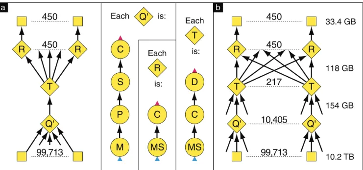
After trying a number of different encapsulation and dy-namic refinement schemes we arrived at the communication graphs shown in Figure 10 for our experiment. Each sub-graph in the first phase now has multiple inputs, grouped automatically using the refinement in Figure 7 to ensure they all lie on the same computer. The inputs are sent to the parserP through a non-deterministic merge vertexM. The distribution (vertexD) has been taken out of the first phase to allow another layer of grouping and aggregation (again using the refinement in Figure 7) before the explo-sion in the number of output channels.

We ran this experiment on 10,160,519,065,748 Bytes of in-put data in a cluster of around 1800 comin-puters embedded in a data center. The input was divided into 99,713 parti-tions replicated across the computers, and we speciﬁed that the application should use 450Rsubgraphs. The ﬁrst phase grouped the inputs into at most 1 GBytes at a time, all ly-ing on the same computer, resultly-ing in 10,405Qsubgraphs that wrote a total of 153,703,445,725 Bytes. The outputs from the Q subgraphs were then grouped into sets of at most 600 MBytes on the same local switch resulting in 217

T subgraphs. EachT was connected to everyR subgraph, and they wrote a total of 118,364,131,628 Bytes. The to-tal output from the Rsubgraphs was 33,375,616,713 Bytes, and the end-to-end computation took 11 minutes and 30 seconds. Though this experiment only uses 11,072 vertices, intermediate experiments with other graph topologies con-ﬁrmed that Dryad can successfully execute jobs containing hundreds of thousands of vertices.

We would like to emphasize several points about the op-timization process we used to arrive at the graphs in Fig-ure 10:

1. At no point during the optimization did we have to modify any of the code running inside the vertices: we were simply manipulating the graph of the job’s communication ﬂow, changing tens of lines of code. 2. This communication graph is well suited to any

map-reduce computation with similar characteristics: i.e. that the map phase (ourP vertex) performs

(11)

substan-Q'

Q'

R

Q'

R

450

T

217

450

10,405

99,713

is:

Each

R

is:

Each

MS

C

T

is:

Each

MS

D

C

M

P

C

S

Q'

R

450

T

450

99,713

33.4 GB

11

8

GB

154 GB

10.2 TB

a

b

Figure 10: Rearranging the vertices gives better scaling performance compared with Figure 9.The user supplies graph (a) specifying that 450 buckets should be used when distributing the output, and that each_Qvertex may receive up to 1GB of input while each_Tmay receive up to 600MB. The number ofQandT vertices is determined at run time based on the number of partitions in the input and the network locations and output sizes of preceding vertices in the graph, and the refined graph (b) is executed by the system. Details are in Section 6.3.

tial data reduction and the reduce phase (ourCvertex) performs some additional relatively minor data reduc-tion. A diﬀerent topology might give better perfor-mance for a map-reduce task with diﬀerent behavior; for example if the reduce phase performed substantial data reduction a dynamic merge tree as described in Figure 6 might be more suitable.

3. When scaling up another order of magnitude or two, we might change the topology again, e.g. by adding more layers of aggregation between theTandRstages. Such re-factoring is easy to do.

4. Getting good performance for large-scale data-mining computations is not trivial. Many novel features of the Dryad system, including subgraph encapsulation and dynamic refinement, were used. These made it simple to experiment with different optimization schemes that would have been difficult or impossible to implement using a simpler but less powerful system.

7.

BUILDING ON DRYAD

As explained in the introduction, we have targeted Dryad at developers who are experienced at using high-level com-piled programming languages. In some domains there may be great value in making common large-scale data process-ing tasks easier to perform, since this allows non-developers to directly query the data store [33]. We designed Dryad to be usable as a platform on which to develop such more re-stricted but simpler programming interfaces, and two other groups within Microsoft have already prototyped systems to address particular application domains.

7.1

The “Nebula” scripting language

One team has layered a scripting interface on top of Dryad. It allows a user to specify a computation as a series of stages (corresponding to the Dryad stages described in Section 3.6),

each taking inputs from one or more previous stages or the ﬁle system. Nebula transforms Dryad into a generalization of the Unix piping mechanism and it allows programmers to write giant acyclic graphs spanning many computers. Often a Nebula script only refers to existing executables such as

perlorgrep, allowing a user to write an entire complex dis-tributed application without compiling any code. The Neb-ula layer on top of Dryad, together with some perl wrap-per functions, has proved to be very successful for large-scale text processing, with a low barrier to entry for users. Scripts typically run on thousands of computers and contain 5–15 stages including multiple projections, aggregations and joins, often combining the information from multiple input sets in sophisticated ways.

Nebula hides most of the details of the Dryad program from the developer. Stages are connected to preceding stages using operators that implicitly determine the number of ver-tices required. For example, a “Filter” operation creates one new vertex for every vertex in its input list, and connects them pointwise to form a pipeline. An “Aggregate” opera-tion can be used to perform exchanges and merges. The im-plementation of the Nebula operators makes use of dynamic optimizations like those described in Section 5.2 however the operator abstraction allows users to remain unaware of the details of these optimizations. All Nebula vertices exe-cute the process wrapper described in Section 4.2, and the vertices in a given stage all run the same executable and command-line, speciﬁed using the script. The Nebula sys-tem deﬁnes conventions for passing the names of the input and output pipes to the vertex executable command-line.

There is a very popular “front-end” to Nebula that lets the user describe a job using a combination of: fragments of

perlthat parse lines of text from diﬀerent sources into struc-tured records; and a relational query over those strucstruc-tured records expressed in a subset of SQL that includesselect,

project and join. This job description is converted into a Nebula script and executed using Dryad. Theperl

(12)

pars-ing fragments for common input sources are all in libraries, so many jobs using this front-end are completely described using a few lines of SQL.

7.2

Integration with SSIS

SQL Server Integration Services (SSIS) [6] supports work-ﬂow-based application programming on a single instance of SQLServer. The AdCenter team in MSN has developed a system that embeds local SSIS computations in a larger, distributed graph with communication, scheduling and fault tolerance provided by Dryad. The SSIS input graph can be built and tested on a single computer using the full range of SQL developer tools. These include a graphical editor for constructing the job topology, and an integrated debugger. When the graph is ready to run on a larger cluster the sys-tem automatically partitions it using heuristics and builds a Dryad graph that is then executed in a distributed fash-ion. Each Dryad vertex is an instance of SQLServer running an SSIS subgraph of the complete job. This system is cur-rently deployed in a live production system as part of one of AdCenter’s log processing pipelines.

7.3

Distributed SQL queries

One obvious additional direction would be to adapt a query optimizer for SQL or LINQ [4] queries to compile plans directly into a Dryad flow graph using appropriate parameterized vertices for the relational operations. Since our fault-tolerance model only requires that inputs be im-mutable over the duration of the query, any underlying stor-age system that offers lightweight snapshots would suffice to allow us to deliver consistent query results. We intend to pursue this as future work.

8.

RELATED WORK

Dryad is related to a broad class of prior literature, rang-ing from custom hardware to parallel databases, but we be-lieve that the ensemble of trade-oﬀs we have chosen for its design, and some of the technologies we have deployed, make it a unique system.

Hardware Several hardware systems use stream program-ming models similar to Dryad, including Intel IXP [2], Imagine [26], and SCORE [15]. Programmers or com-pilers represent the distributed computation as a col-lection of independent subroutines residing within a high-level graph.

Click A similar approach is adopted by the Click modular router [27]. The technique used to encapsulate multi-ple Dryad vertices in a single large vertex, described in section 3.4, is similar to the method used by Click to group the elements (equivalent of Dryad vertices) in a single process. However, Click is always single-threaded, while Dryad encapsulated vertices are de-signed to take advantage of multiple CPU cores that may be available.

Dataflow The overall structure of a Dryad application is closely related to large-grain dataﬂow techniques used in e.g. LGDF2 [19], CODE2 [31] and P-RIO [29]. These systems were not designed to scale to large clusters of commodity computers, however, and do not toler-ate machine failures or easily support programming very large graphs. Paralex [9] has many similarities

to Dryad, but in order to provide automatic fault-tolerance sacriﬁces the vertex programming model, al-lowing only pure-functional programs.

Parallel databases Dryad is heavily indebted to the tra-ditional parallel database ﬁeld [18]: e.g., Vulcan [22], Gamma [17], RDb [11], DB2 parallel edition [12], and many others. Many techniques for exploiting paral-lelism, including data partitioning; pipelined and par-titioned parallelism; and hash-based distribution are directly derived from this work. We can map the whole relational algebra on top of Dryad, however Dryad is not a database engine: it does not include a query planner or optimizer; the system has no concept of data schemas or indices; and Dryad does not sup-port transactions or logs. Dryad gives the program-mer more control than SQL via C++ programs in ver-tices and allows programmers to specify encapsulation, transport mechanisms for edges, and callbacks for ver-tex stages. Moreover, the graph builder language al-lows Dryad to express irregular computations.

Continuous Query systems There are some superﬁcial similarities between CQ systems (e.g. [25, 10, 34]) and Dryad, such as some operators and the topologies of the computation networks. However, Dryad is a batch computation system, not designed to support real-time operation which is crucial for CQ systems since many CQ window operators depend on real-time behavior. Moreover, many datamining Dryad computations re-quire extremely high throughput (tens of millions of records per second per node), which is much greater than that typically seen in the CQ literature.

Explicitly parallel languages like Parallel Haskell [38], Cilk [14] or NESL [13] have the same emphasis as Dryad on using the user’s knowledge of the problem to drive the parallelization. By relying on C++, Dryad should have a faster learning curve than that for func-tional languages, while also being able to leverage com-mercial optimizing compilers. There is some appeal in these alternative approaches, which present the user with a uniform programming abstraction rather than our two-level hierarchy. However, we believe that for data-parallel applications that are naturally written using coarse-grain communication patterns, we gain substantial beneﬁt by letting the programmer cooper-ate with the system to decide on the granularity of distribution.

Grid computing [1] and projects such as Condor [37] are clearly related to Dryad, in that they leverage the re-sources of many workstations using batch processing. However, Dryad does not attempt to provide support for wide-area operation, transparent remote I/O, or multiple administrative domains. Dryad is optimized for the case of a very high-throughput LAN, whereas in Condor bandwidth management is essentially handled by the user job.

Google MapReduce The Dryad system was primarily de-signed to support large-scale data-mining over clusters of thousands of computers. As a result, of the recent related systems it shares the most similarities with Google’s MapReduce [16, 33] which addresses a similar

(13)

problem domain. The fundamental diﬀerence between the two systems is that a Dryad application may spec-ify an arbitrary communication DAG rather than re-quiring a sequence of map/distribute/sort/reduce op-erations. In particular, graph vertices may consume multiple inputs, and generate multiple outputs, of dif-ferent types. For many applications this simpliﬁes the mapping from algorithm to implementation, lets us build on a greater library of basic subroutines, and, together with the ability to exploit TCP pipes and shared-memory for data edges, can bring substantial performance gains. At the same time, our implemen-tation is general enough to support all the features described in the MapReduce paper.

Scientific computing Dryad is also related to high-perfor-mance computing platforms like MPI [5], PVM [35], or computing on GPUs [36]. However, Dryad focuses on a model with no shared-memory between vertices, and uses no synchronization primitives.

NOW The original impetus for employing clusters of work-stations with a shared-nothing memory model came from projects like Berkeley NOW [7, 8], or TACC [20]. Dryad borrows some ideas from these systems, such as fault-tolerance through re-execution and central-ized resource scheduling, but our system additionally provides a uniﬁed, simple high-level programming lan-guage layer.

Log datamining Addamark, now renamed SenSage [32] has successfully commercialized software for log data-mining on clusters of workstations. Dryad is designed to scale to much larger implementations, up to thou-sands of computers.

9.

DISCUSSION

With the basic Dryad infrastructure in place, we see a number of interesting future research directions. One fun-damental question is the applicability of the programming model to general large-scale computations beyond text pro-cessing and relational queries. Of course, not all programs are easily expressed using a coarse-grain data-parallel com-munication graph, but we are now well positioned to identify and evaluate Dryad’s suitability for those that are.

Section 3 assumes an application developer will first con-struct a static job graph, then pass it to the runtime to be executed. Section 6.3 shows the benefits of allowing applica-tions to perform automatic dynamic refinement of the graph. We plan to extend this idea and also introduce interfaces to simplify dynamic modifications of the graph according to application-level control flow decisions. We are particularly interested in data-dependent optimizations that might pick entirely different strategies (for example choosing between in-memory and external sorts) as the job progresses and the volume of data at intermediate stages becomes known. Many of these strategies are already described in the paral-lel database literature, but Dryad gives us a flexible testbed for exploring them at very large scale. At the same time, we must ensure that any new optimizations can be targeted by higher-level languages on top of Dryad, and we plan to implement comprehensive support for relational queries as suggested in Section 7.3.

The job manager described in this paper assumes it has exclusive control of all of the computers in the cluster, and this makes it difficult to efficiently run more than one job at a time. We have completed preliminary experiments with a new implementation that allows multiple jobs to cooper-ate when executing concurrently. We have found that this makes much more efficient use of the resources of a large cluster, but are still exploring variants of the basic design. A full analysis of our experiments will be presented in a future publication.

There are many opportunities for improved performance monitoring and debugging. Each run of a large Dryad job generates statistics on the resource usage of thousands of ex-ecutions of the same program on diﬀerent input data. These statistics are already used to detect and re-execute slow-running “outlier” vertices. We plan to keep and analyze the statistics from a large number of jobs to look for patterns that can be used to predict the resource needs of vertices before they are executed. By feeding these predictions to our scheduler, we may be able to continue to make more eﬃcient use of a shared cluster.

Much of the simplicity of the Dryad scheduler and fault-tolerance model come from the assumption that vertices are deterministic. If an application contains non-deterministic vertices then we might in future aim for the guarantee that every terminating execution produces an output that some failure-free execution could have generated. In the general case where vertices can produce side-eﬀects this might be very hard to ensure automatically.

The Dryad system implements a general-purpose data-parallel execution engine. We have demonstrated excellent scaling behavior on small clusters, with absolute perfor-mance superior to a commercial database system for a hand-coded read-only query. On a larger cluster we have executed jobs containing hundreds of thousands of vertices, process-ing many terabytes of input data in minutes, and we can automatically adapt the computation to exploit network lo-cality. We let developers easily create large-scale distributed applications without requiring them to master any concur-rency techniques beyond being able to draw a graph of the data dependencies of their algorithms. We sacriﬁce some architectural simplicity compared with the MapReduce sys-tem design, but in exchange we release developers from the burden of expressing their code as a strict sequence of map, sort and reduce steps. We also allow the programmer the freedom to specify the communication transport which, for suitable