University of California, Berkeley
U.C. Berkeley Division of Biostatistics Working Paper Series
Year Paper
Collaborative Targeted Maximum Likelihood
For Time To Event Data
Ori M. Stitelman
∗Mark J. van der Laan
†∗University of California - Berkeley, [email protected]
†University of California - Berkeley, [email protected]
This working paper is hosted by The Berkeley Electronic Press (bepress) and may not be commer-cially reproduced without the permission of the copyright holder.
http://biostats.bepress.com/ucbbiostat/paper260
Collaborative Targeted Maximum Likelihood
For Time To Event Data
Ori M. Stitelman and Mark J. van der Laan
Abstract
Current methods used to analyze time to event data either, rely on highly paramet-ric assumptions which result in biased estimates of parameters which are purely chosen out of convenience, or are highly unstable because they ignore the global constraints of the true model. By using Targeted Maximum Likelihood Estima-tion one may consistently estimate parameters which directly answer the statistical question of interest. Targeted Maximum Likelihood Estimators are substitution estimators, which rely on estimating the underlying distribution. However, unlike other substitution estimators, the underlying distribution is estimated specifically to reduce bias in the estimate of the parameter of interest. We will present here an extension of Targeted Maximum Likelihood Estimation for observational time to event data, the Collaborative Targeted Maximum Likelihood Estimator for the treatment specific survival curve. Through the use of a simulation study we will show that this method improves on commonly used methods in both robustness and efficiency. In fact, we will show that in certain situations the C-TMLE pro-duces estimates whose mean square error is lower than the semi-parametric effi-ciency bound. Lastly, we will show that the bootstrap is able to produce valid 95 percent confidence intervals in sparse data situations, while influence curve based inference breaks down.
1
Introduction
It is common to want to quantify in observational data the effect of a treatment or ex-posure on the time it takes for an event to occur. In Moore and van der Laan 2009 they introduce the targeted maximum likelihood estimator for estimating the treatment spe-cific survival curve in randomized clinical trials [2]. The targeted maximum likelihood estimator (TMLE) presented there improves upon common methods for analyzing time to event data in robustness, efficiency, and interpretability of parameter estimates. However, those methods may not be directly applied to observational data because it differs from randomized clinical trials in that the exposure/treatment is not set externally.
A 2009 paper by van der Laan and Gruber introduces a new class of estimators, the col-laboratively double robust targeted maximum likelihood estimators (C-TMLE)[8]. These estimators are an extension of TMLE specific to the observational setting. The C-TMLE methods presented there provide estimates which, in many instances, are more efficient than standard TMLE and all other possible estimation techniques. In fact, the C-TMLE may produce super efficient estimates, or estimates which are more efficient than the semi-parametric efficiency bound. Furthermore, the C-TMLE methodology produces well be-haved estimates in situations where the parameter of interest is borderline identifiable. When exposure is not randomized there may be individuals with certain baseline charac-teristics which never experience a particular level of exposure. In other words, a certain set of baseline characteristics may be completely predictive of a particular treatment level. This phenomenon is termed a violation in the experimental treatment assumption (ETA) in Neugebauer and van der Laan 2005 [3]. Violations in ETA render the parameters of interest as presented in Moore and van der Laan unidentifiable. However, many times in finite samples certain parameters are weakly identifiable due to practical violations in the ETA assumption. Practical violations occur when a certain set of baseline covariates are almost completely predictive of a certain treatment within the sample. C-TMLE estima-tors address this issue and are able to produce stable estimates of borderline identifiable parameters. Thus, the C-TMLE methodology may be applied in the time to event setting to gain efficiency as well as produce estimates for weakly identifiable parameters of interest. van der Laan and Gruber present a general methodology for constructing C-TMLE esti-mators as well as apply the method to several basic data structures. We will extend those methods to time to event data and present a C-TMLE methodology for estimating the treatment specific survival curve. A simulation study will also be presented that illustrates the advantages of using C-TMLE versus other methods.
2
Estimating Parameters In Coarsened Data Structures
In this section we will briefly introduce the parameter estimation problem for a coarsened data structure. Then different methods for estimating parameters within this data struc-ture will be introduced along with their shortcomings. Finally, we will discuss the TMLE
methodology in general, and illustrate how the properties of targeted maximum likelihood estimates address the drawbacks seen in the other estimators.
Suppose one observes a censored data structure O = Φ(C, X) of the full data X and censoring variableC which has a probability distribution P0. LetMbe a semiparametric model for the probability distributionP0. By assuming coarsening at random (CAR) the density factors asdP0(O) =Q0(O)g0(O|X), whereQ0 is the part of the density associated with the full data,X, andg0 is the conditional distribution of the observed data,O, given the full data. g0 includes both the censoring and treatment mechanism, which both act to coarsen the full data. The factorization of the density implies that the modelM may be partitioned into a modelQfor the full data distribution,Q0, and modelG for the censoring and treatment mechanism, g0. So the probability distribution, P0 may be indexed in the following way: PQ0,g0. One is typically interested in estimating a parameter, Ψ(P0), which is a function of the true data generating distribution. More specifically, the parameter of interest is Ψ(Q0) which is a function of the true full data generating distribution absent coarsening.
Many methods have been developed to estimate Ψ(Q0). Traditional maximum like-lihood estimation methods approach this problem by producing a substitution estimator Ψ( ˆQ), where maximum likelihood is used to estimate ˆQ. Since the model Mcan be very large, this would require sieve-based (data adaptive) maximum likelihood estimation (i.e., loss-based machine learning), involving fine-tuning of the amount of smoothing used.1 If Ψ(Q0) denotes a causal effect, this estimator is referred to as the G-computation estima-tor (G-comp). Such methods typically produce overly biased estimates of the parameter of interest since the estimate of Q0 is at best created with concern for the bias variance trade off of the entire density rather than for the parameter of interest. However, the G-comp estimator does respect the global constraints of the model by acknowledging that the parameter of interest is is a function of Q0, Ψ(Q0). Thus, the estimate, ˆψgcomp, is a substitution of a maximum likelihood estimator, ˆQ in the model Q, into the parameter mapping Ψ(). In addition, by using state of the art loss (log-likelihood) based learning, it provides low-variance estimators, inspired by the efficient parametric maximum likelihood estimation.
An alternative method for estimating Ψ(Q0) is the inverse probability of treatment based approach (IPW). IPW estimators solve an estimating equation in order to yield estimates, ˆψIP W, of the parameter of interest. ˆψIP W are consistent estimates of Ψ(Q0) when one estimates theg part of the likelihood consistently. However, IPW estimates are highly unstable for two reasons. First, IPW estimates do not solve the efficeint influence curve estimating equation. Second, they do not respect the global restraints of a proper
1
A detailed account of loss based learning and cross validation may be seen in van der Laan and Dudoit 2003 [6]. In addition, van der Laan, Keles and Dudoit focus specifically on likelihood-based cross-validation and illustrate its asymptotic optimality in their 2004 article [7]. van der Laan, Polley, and Hubbard rely on the results of the previous two papers in their 2007 article which presents the Super Learner methodology, a data-adaptive learning technique which utilizes likelihood based cross-validation[9].
model by being a substitution estimator. As a result IPW estimates are highly variable and act erratically in finite samples.
Another method for estimating Ψ(Q0) is augmented inverse probability weighted esti-mators (AIPW). Robins and Rotntizky proposed this general estimating equation based approach in 1992 which constructs estimators, ˆψAIP W, that solve the efficient influence curve estimating equation [5]. The estimates produced by these methods are referred to as double robust because they are consistent when either theQor theg part of the likeli-hood are estimated consistently. Furthermore, they also improve on the standard inverse probability weighted estimators in terms of efficiency since they solve the efficient influence curve equation; thus, they are locally efficient. However, like the IPW estimators, the AIPW estimators are not substitution estimators and may also be unstable. For a general treatment of these methods see Robins and van der Laan 2003 [10].
van der Laan and Rubin in their 2006 paper introduce a new class of estimators, the targeted maximum likelihood estimators (TMLE) [11]. The TMLE methodology developed in that paper is a two stage process which results in a substitution estimator. In the first stage an initial estimate, ˆQ0, of Q0 is obtained, using loss-based learning. In the second stage the first stage estimate is fluctuated to reduce bias in the estimate of the parameter of interest. The bias is reduced by insuring that the efficient influence curve equation is solved by the targeted maximum likelihood solution ˆQ∗. This is achieved by finding the targeted maximum likelihood estimate ofQ0, ˆQ∗g, with a parametric fluctuation model whose score at the initial estimator (i.e., at zero fluctuation) equals or includes the efficient influence curve of the parameter of interest. This may be done by specifying a univariate regression model for the outcome of interest on a covariate,h( ˆQ0,gˆ), specifically chosen to yield the appropriate score while using the initial estimator of ˆQ0 as an offset. h( ˆQ0,gˆ) is a function of ˆg and thus the second stage requires an estimate ˆg of g0. The coefficient in front of the clever covariate, h( ˆQ0,gˆ), is then estimated using standard parametric maximum likelihood. This is known as the first targeted maximum likelihood step and yields ˆQ1, the first step targeted maximum likelihood estimate ofQ0. The targeted maximum likelihood step is then iterated using ˆQ1 as the initial estimator ofQ0 and the estimate of g0 remains unchanged. This process is iterated until converges to zero, resulting in the targeted maximum likelihood estimate of Q0, or ˆQ∗g. Ψ( ˆQ∗g) is the targeted maximum likelihood estimate of the parameter Ψ(Q0). Note, that ˆQ∗g is indexed by the treatment and censoring mechanisms, g. This is because unlike the G-computation estimators above, the TMLE, throughh, makes use of the fact that the observed data is generated according to a censored data structure as dictated by the efficient influence curve for Ψ(Q0).
Like the AIPW estimators the TMLE estimates are double robust and locally efficient; however, the TMLE methedology improves on the AIPW approach that also solves the efficient influence curve equation in four major ways:
1. The TMLE respects the global constraint of the model and the AIPW estimate does not. Since the TMLE is a substitution estimator and maps the targeted maximum
likelihood estimate ˆP∗ofP0into the parameter mapping Ψ(), it respects knowledge of the model. By solving an estimating equation, AIPW estimators, in most instances, do not acknowledge that one is estimating a parameter which is a function of the underlying data generating distribution. One situation where this issue is glaringly obvious is when AIPW estimators can return estimates which are out of the natural bounds of the problem, as is the case when one is estimating a probability that must fall between 0 and 1. However, the implications of respecting the knowledge of the model are more subtle than just returning estimates which are out of the natural bounds of the parameter and this advantage contributes to finite sample gains in efficiency which will be displayed in the simulation results presented below, and are particularly strong in the context of sparsity w.r.t. the target parameter (i.e., the sample contains sparse information about the parameter of interest).
2. The log-likelihood of ˆQ∗g, or targeted maximum likelihood, is a direct measure of fit upon which to choose among different estimates of g and Q. Prior to TMLE, estimators which relied on estimates of Q and g to identify PQ0,g0 distinguished between different estimates based on how well they do for prediction by using a loss function for the global density. Whereas, the TMLE methedology uses the targeted maximum likelihood to choose among different estimates based on how they help in estimating the parameter of interest, Ψ(Q0). This advantage is particularly striking in the typical context that there are excellent fits of g0 itself, resulting in unstable inverse of probability of censoring weights, that truly harm the bias reduction effort for the target parameter ofQ0.
3. The TMLE can produce estimates when the efficient influence curve may not be written as an estimating function in terms of the parameter of interest,ψ. The AIPW estimate requires that the efficient influence curve be represented as an estimating function. The log-rank parameter, as presented in Moore and van der Laan 2009, is an example of a parameter whose efficient influence curve may not be written as an estimating function and thus can be estimated directly through TMLE but not directly by AIPW estimators.
4. The TMLE does not have multiple solutions. Since AIPW estimates are solutions to estimating equations they may have multiple solutions. The estimating equation itself provides no criteria upon which to choose between the multiple solutions. TMLE does not suffer from multiple solutions since it is a loss-based learning approach, e.g., maximizing the log-likelihood fit, involving second stage extra fitting along a target-parameter specific parametric fluctuation model, which just happens to also solve the efficient influence curve estimating equationin the probability distribution.
How these advantages, specifically the first two, actually effect the properties of the esti-mates produced by the TMLE methedology will be explored in the following sections and
be quantified in comparison to other methods through a simulation study presented in sections 12 through 14.
3
Collaborative Targeted Maximum Likelihood Estimation
In General
In their original paper on C-TMLE van der Laan and Gruber introduce a new and stronger type of double robustness entitled collaborative double robustness. The collaboratively double robustness property of an (targeted ML) estimator ˆQˆg of Q0 only requires that the estimate of g0, ˆg, account for variables that effect Q0 and were not fully accounted for in the initial ˆQ. Thus the property does not require that either the estimates of Qor g are consistent, but rather is concerned with reducing the distance between, ˆQˆg andQ0, and, ˆg and g0, such that the resulting estimator of Ψ(Q0) is unbiased. So if ˆQ does a very good job estimating Q0, very little adjustment is necessary through the estimate of g; on the other hand, if ˆQ is a poor estimate of Q0, the estimate ˆg will have to do a better job of estimatingg0 with respect to those variables that effect Q0.
The C-TMLE methodology, introduced by van der Laan and Gruber, is an extension of TMLE that takes advantage of the collaborative doubly robust property of those estimators by constructing ˆg in collaboration with ˆQ. C-TMLE uses the log-likelihood as a loss function to choose from a sequence of K targeted maximum likelihood estimates, ˆQk∗, indexed by initial estimates of Q0 and g0. In their paper, van der Laan and Gruber provide a framework for generating C-TMLEs which we will briefly outline now:
1. Create ˆQ, an initial estimator of Q0.
2. Generate a sequence of estimates of g0: ˆg0,gˆ1, . . . ,gˆK−1,gˆK. Where ˆg0 is the least data adaptive estimate and ˆgK is the most data adaptive estimate ofg
0. 3. Generate the initial TMLE estimate, ˆQ0∗, indexed by ˆQand ˆg0.
4. Generate a sequence of TMLE estimates: ˆQ0∗,Qˆ1∗. . . ,QˆK−1∗,QˆK∗ indexed by ˆgk; where each estimate has a larger log-likelihood than the last. This monotonicity is insured by adding an additional clever covariate to estimate ˆQk∗ each time the log-likelihood does not increase within the same clever covariate just by virtue of the more data adaptive estimate ofg. Whenever a new clever covariate is added for ˆQk∗,
ˆ
Qk−1∗ is used as the initial estimate in the TMLE algorithm.
5. Finally, choose among the sequence of TMLE estimates using loss based cross-validation with log-likelihood loss.
One adjustment to the above methodology, suggested by van der Laan and Gruber, is to use a penalized loss function when parameters are borderline identifiable. This is a very
important consideration in observational studies and the issue of choosing an appropriate penalty is addressed in section 6.
The C-TMLE has two distinct advantages over the TMLE methodology:
1. C-TMLE may be used to produce stable estimates of borderline identifiable parame-ters while TMLE (or any of the estimating equation methods discussed above) break-down in these situations. The reason many parameters are not identifiable, or are borderline identifiable, is due to violations in ETA, where a certain level of a co-variate or group of coco-variates is completely predictive of treatment/exposure. In these situations, where sparsity of the data is an issue, C-TMLE is able to weigh the bias-variance trade off of adjusting for certain covariates in estimating these weakly identifiable parameters. Thus, C-TMLE only adjusts for covariates in estimating
g0 when they are beneficial to the estimate of the parameter of interest and selects against adjusting for covariates which are detrimental to the final estimate of Ψ(Q0), weighing both bias and variance. All other methods estimateg0 using a loss function for prediction, ora priori specifying a model, ignoring the effect adjusting for certain covariates has on the final estimate of the parameter of interest.
2. C-TMLE estimates in many situations are more efficient in finite samples than TMLE estimates. In fact, in some situations they are super-efficient and have a variance smaller than the semi-parametric efficiency bound. This is also a consequence of the collaborative double robustness of these estimates. In situations where the initial estimate, ˆQ is a very good estimate of Q0 in the targeted sense little adjustment is needed from the estimate ofg0. The more one adjusts forgthe larger the variability of the final estimate of the parameter of interest and thus not adjusting much ingwhen one doesn’t have to provides estimates with smaller variance. In some rare situations C-TMLE estimates have also been shown to be asymptotically super efficient: for example, if the initial estimator ˆQ is a MLE for a correctly specified parametric model.
The C-TMLE estimates exhibit all of the advantages of the TMLE estimates discussed in the previous section as well as these two major advantages presented here. The advan-tages of C-TMLE estimators are particularly useful in observational studies, where practical violations in the ETA assumption are a concern; however, in studies where treatment is randomized and one attempts to gain efficiency by estimating g C-TMLE estimators are also appropriate because they address the bias variance trade off of adjusting for particular variables.2 Thus, implementation of the C-TMLE methods even for randomized treat-ments will help insure that one does not adjust ingfor the covariates in a way that hinders the estimate of the parameter of interest. In the following sections we will use a specific coarsened data structure, time to event data, to exhibit the advantages of C-TMLE.
2For a general account of how estimating the nuisance parameter mechanism even when it is known contributes to a gain in efficiency see van der Laan and Robins (2003), Section 2.3.7.
4
Data Structure
Time to event analyses typically intend to assess the causal effect of a particular exposure,
A, on the time, T, it takes for an event to occur. However, many times subjects are lost to follow up and as a result T is not observed for all individuals. Individuals for whom the event is not observed are referred to as censored. This type of censoring is called right censoring since chronological time is arbitrarily chosen to progress from left to right and at some point in time,C, an individual is no longer observed; thus, all time points to the right ofC are censored for that individual. Some baseline covariates,W, are also recorded for each individual.
The observed data consists of n i.i.d copies of,O =
A, W,T ,˜ ∆
. WhereA, is a binary variable, which quantifies the level of exposure/treatment a particular subject experiences,
W is a vector of baseline covariates, ˜T is the last time point at which a subject is observed, and ∆ indicates whether the event occurred at ˜T. So ˜T =min(T, C) and ∆ =I(T ≤C), whereC is the time at which a subject is censored. If the event is observed, ∆ = 1, andC
is set equal to ∞. Alternatively if the event is not observed, ∆ = 0, and T is set equal to
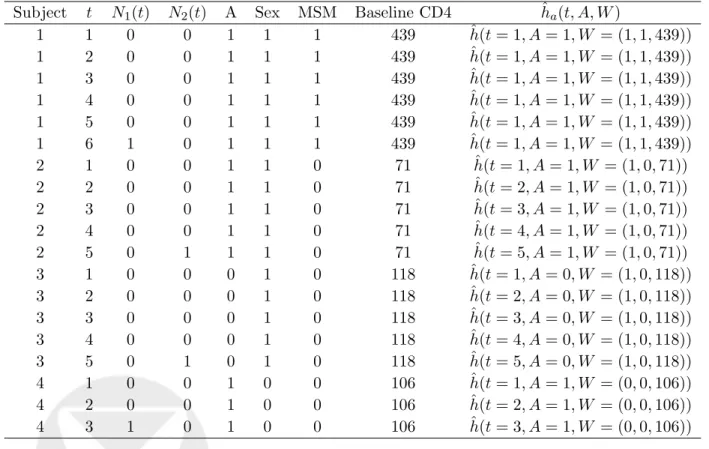
∞. This formulation of the data structure is termed the short form of survival data and includes a row in the data set for each subject observed. Table 1 presents as an example four observations with selected baseline covariates from a sample HIV data set in their short form.
Subject T˜ ∆ A Sex MSM Baseline CD4
1 6 1 1 1 1 439
2 5 0 1 1 0 71
3 5 0 0 1 0 118
4 3 1 1 0 0 106
Table 1: Example of sample HIV data in short form.
Alternatively, one may represent the same data in its long form. In this form the data set includes a row for each observation for each time the subject is observed up until it is either censored or experiences the event of interest. In order to represent the data in its long form two additional random variables must be introducedN1(t) and N2(t), where the first is an indicator that the event happens at time t, and the second is an indicator that a subject is censored at time t. Thus, subject 1 would have six rows in the data set in its long form and N1(t) will equal zero in every row except for the last row at t = 6 and N2(t) will equal zero in each row. Table 2 displays the same four observations from Table 1 in their long form. The baseline values, A and W, are repeated at each time point for each subject. Presenting the data in its long form allows for more flexibility and is essential for representing a general time dependent process (e.g., when dealing with time dependent covariates, variables whose value change over time, and/or counting processes
that can jump more than once). In fact, it will be shown below that estimating TMLEs involves construction of a time dependent covariate, since h( ˆQ,ˆg) is a function of t, A, and W and can be written as h(t, A, W). So the data in its long form is n i.i.d. copies of
O=
A, W, N1(t), N2(t) :t= 1, . . . ,T˜
∼p0, wherep0denotes the density of the observed data, O.
Subject t N1(t) N2(t) A Sex MSM Baseline CD4
1 1 0 0 1 1 1 439 1 2 0 0 1 1 1 439 1 3 0 0 1 1 1 439 1 4 0 0 1 1 1 439 1 5 0 0 1 1 1 439 1 6 1 0 1 1 1 439 2 1 0 0 1 1 0 71 2 2 0 0 1 1 0 71 2 3 0 0 1 1 0 71 2 4 0 0 1 1 0 71 2 5 0 1 1 1 0 71 3 1 0 0 0 1 0 118 3 2 0 0 0 1 0 118 3 3 0 0 0 1 0 118 3 4 0 0 0 1 0 118 3 5 0 1 0 1 0 118 4 1 0 0 1 0 0 106 4 2 0 0 1 0 0 106 4 3 1 0 1 0 0 106
Table 2: Example of sample HIV data in long form.
5
Causal Assumptions and Factorization Of Observed Data
Likelihood
The data structure presented in the preceding section implies little about the causal ture of the underlying mechanisms which produce the observed data. The temporal struc-ture which is implied by the fact thatA and W are measured at baseline and then some time in the future, T, an event occurs is clear from the observed data structure; however, no assumptions have been made as to howAeffects the outcome,T. DoesAdirectly effect
T? DoesAeffectW which then effectsT? DoesAeffectT through W as well as directly? Does A even cause W or does W cause A? In fact, there are countless numbers of ways
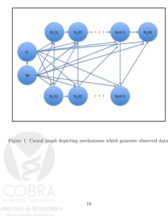
which the observed random variables could have caused or been caused by each other. In order to quantify, or even define, the causal effect of A on the outcome T causal assump-tions are necessary. Causal graphs succinctly lay out the causal assumpassump-tions necessary to define a causal effect as well as provide much of the information needed to determine if the effect is estimable from the observed data. For a detailed account of causal graph theory see Pearl 2008 [4]. One constructs a causal graph based on the cues provided from the world in which the observed phenomenon are occurring, whether it be based on subject knowledge or constraints imposed by how an experiment is designed.3 Such issues are out of the scope of this paper and we will just assume that the causal graph presented in Figure 1 depicts the data generating mechanisms for the observed data. Exogenous error nodes, whose joint distribution is such that there are no unblocked backdoor paths from A and theN1(t) nodes to any of theN2(t) nodes of the event process, are suppressed in the causal graph, as is typically done in the literature. Thus, each node is defined in the causal graph as a function of its ancestors and an exogenous error node which is not depicted in the graph.
The causal graph depicted in Figure 1 presents a common structure for which one may be interested in the causal effect ofA on the time until an event occurs. This causal structure corresponds with the causal structure examined in Moore and van der Laan 2009, except for the fact thatW now is a direct cause of A, indicated by an arrow from W to
A. This change is due to the fact that Ais not externally set as in a randomly controlled experiment, but rather, is free to be whatever it would be as naturally observed. Thus, other variables,W, effect what level ofAa subject experiences.
The causal graph allows one to make necessary assumptions typically stated to make causal parameters estimable. The consistency assumption, and coarsening at random as-sumption are made directly by the causal graph. The consistency asas-sumption states that the observed outcome is the counterfactual outcome under the intervention actually ob-served. This assumption is a direct consequence of defining each node in the causal graph as a function of its ancestors and exogenous error nodes, and defining the observed data
O as the observed nodes generated by the nonparametric structural equation model rep-resented by the causal graph. The coarsening at random assumption (CAR) states that the coarsening mechanism is only a function of the full data, the data in which you would have seen all counterfactuals, through the observed data. For the treatment variable this assumption is sometimes referred to as the randomization assumption or no unmeasured confounders assumption. This is directly implied by the causal graph since the treatment and censoring process variables only have arrows into them from their observed ancestors and no other nodes. This may also be confirmed by applying the no unblocked backdoor path criteria presented by Pearl [4].
3
Pearl 2008 discusses algorithms which can search over observed data and provide a set of causal graphs which are consistent with that data. This use of causal graph theory is not consistent with our goal. For our purposes the causal graph is used to succinctly impose causal assumptions which we are able to make based off of knowledge of the mechanisms at work.
N1(1) A W N2(1) N1(2) N2(2) N1(K‐1) N2(K‐1)
. . .
. . .
N1(K)The causal graph presented in Figure 1 suggests the following orthogonal factorization of the likelihood of the observed data:
L(O) = Q10 z }| { P(W) g10 z }| { P(A|W) K Y t=1 Q20 z }| { P(N1(t)|N1(t−1), N2(t−1), A, W) (1) P(N2(t)|N1(t), N2(t−1), A, W) | {z } g20
Thus, the likelihood factorizes as the general censored data structure presented in section 2 into a portion corresponding to the full data distribution,Q0, and a portion corresponding to the censoring and treatment mechanism, g0. Q0 is composed of the baseline covariate distribtion,Q10(W) andQ20(t, A, W)≡E(dN1(t)|N1(t−1) = 0, N2(t−1) = 0, A, W), the intensity of the event counting process given the treatment,A, and the baseline covariates,
W, conditioning on “no event yet”. g0 is further factorized into the treatment mechanism,
g10(A, W), and censoring mechanism, g20(t, A, W) ≡ E(dN2(t) | N1(t) = 0, N2(t−1) = 0, A, W), which is the intensity of the censoring process given treatment,A, and the baseline covariates,W, conditioning on “no event yet”. Let’s also define S0(tk |A, W) =P r(T >
tk | A, W) which is the conditional survival of the event of interest corresponding to the intensity of the event process,Q20(t, A, W), under the coarsening at random assumption:
S0(tk |A, W) = tk Y
t=1
[1−Q20(t, A, W)]. (2)
Note thatQ20(t, A, W) is the conditional hazard ofT att, givenA, W, under CAR, which holds if T and Care conditionally independent, givenA, W (and was implied by our causal graph).
6
Parameter of Interest
Now that the likelihood of the data generating distribution has been introduced, parameters of interest which are functions of the data generating distribution, Ψ(p0), may be defined. Defining the parameter of interest as a mapping from the data generating distribution allows one to estimate exactly the feature of the data generating distribution that they are interested in. The treatment specific survival curve at a particular time point,tk, is a simple example of this type of parameter,P r(Ta> tk). WhereTais the event time,T, one would have observed had an individual been set to treatment level a. This type of intervention in the real world may now be ”observed” in our model as an intervention on the causal graph which sets an individual to level A = a. Since we are dealing with time to event data it is also necessary to intervene on the censoring mechanism at each time by setting the individual to uncensored, orN2(t) = 0. These interventions on the nodes associated with theg part of the likelihood in the causal graph allow one to assess the distribution of
the outcome had individuals been set to particular levels of treatment/exposure which are of interest in a world without censoring.
By intervening on the causal graph in Figure 1 by setting treatment A equal to the desired treatment and setting N2(t) to no censoring one may ”observe” the event process under the desired treatment and without censoring. This outcome under the proposed intervention is known as the counterfactual outcome. Based on the causal assumptions imposed by the causal graph we can now write the treatment specific survival probability in terms of the data generating distribution,p0:
Ψa(p0)(tk) = P r(Ta> tk) =EW(S0(tk |A=a, W)). (3) Parameters which combine Ψ1(p0)(tk) and Ψ0(p0)(tk) allow one to quantify the effect of a A on survival, T. Three examples of these types of parameters are the marginal additive difference in the probability of survival, the relative risk of survival, and the log of the marginal relative log hazard of survival:
ΨRD(p0)(tk) = Ψ1(p0)(tk)−Ψ0(p0)(tk), (4) ΨRR(p0)(tk) = Ψ1(p0)(tk) Ψ0(p0)(tk) , (5) ΨRH(p0)(tk) = log log(Ψ1(p0)(tk)) log(Ψ0(p0)(tk)) . (6)
Parameters which average these quantities over a set of time points may also be of interest. For the simulation study presented below we will just focus on the treatment specific survival curve at a particular time point.
7
Alternative Methods For Estimating The Treatment
Spe-cific Survival
In this section we will briefly introduce the G-comp, IPW, and AIPW estimators for the treatment specific survival curve.4 These three alternatives will then be compared to the TMLE/C-TMLE estimates in the simulation study presented in Section 11.
4
It is also common in analyses that intend to test weather or not a treatment or exposure, A, has an effect on a particular time to event outcome, to a priori specify a parametric model of the hazard,
Q20(N1(t), A, W), and to test if the coefficient on A in the specified model is different from zero. For continuous time a cox proportional hazard model is typically employed and for discrete time outcomes a logistic failure time model is used. Such methods are not examined here because they rely on highly parametric assumptions which typically result in biased estimates of parameters which are purely chosen out of convenience.
G-computation estimators are one class of estimators for estimating the mean counter-factual outcome as expressed in the parameters proposed above. G-computation estimators are substitution estimators and thus require an estimate of the data generating distribu-tion. In particular, the estimators require an estimate of the marginal distribution of W,
Q10(W), and the conditional hazard, which is Q20(t, A, W) under an assumption of coars-ening at random. G-computation estimators of the parameter of interest, Ψ, are consistent when these distributions are estimated consistently. The marginal distribution of W is estimated non-parametrically by the empirical distribution of the baseline covariates in the sample. Super Learner, a data-adaptive machine learning algorithm which uses likelihood-based cross validation to choose among a library of different learners is a good method for estimatingQ20and subsequently obtaining ˆS(tk|A, W) [9]. The G-Computation estimate of the treatment specific survival, Ψa(p0)(tk), may be expressed as:
ˆ ψg−compa = 1 n n X i=1 ˆ S(tk|A=a, Wi). (7) The IPW method for estimating the treatment specific survival curve only relies on estimates of theg part of the likelihood. This estimator is an estimating equation based estimator and takes the following form:
ˆ ψaIP W = 1 n n X i=1 I(T > tk)I(C > tk)I(A=a) ˆ g1(a|W)Qti=1− [1−gˆ20(i|A, W)] . (8)
The AIPW estimator is a double robust estimator which solves the efficient influence curve based estimating equation. Thus, this estimator requires both estimates of theQand
g factors of the likelihood. The efficient influence curve for the treatment specific survival curve for this observed data structure is:
D∗a(p0) = X t≤tk ha(t, A, W)hI( ˜T =t,∆ = 1)−I( ˜T ≥t)Q20(t, A=a, W)i (9) +S0(tk|A= 1, W) + Ψa(p0)(tk), where ha(t, A, W) =− I(A=a) g10(A=a|W)Qt− i=1[1−g20(i|A, W)] S0(tk|A, W) S0(t|A, W) I(t≤tk) (10) Hubbard et al. develop the one-step AIPW estimator which solves the efficient influence curve estimating equation in their 1999 paper [1]. The resulting AIPW estimate is:
ˆ ψAIP Wa = 1 n n X i=1 X t≤tk ˆ ha(t, A, W) h I( ˜T =t,∆ = 1)−I( ˜T≥t) ˆQ2(N1(t) = 1, A=a, W) i + ˆS(tk|A= 1, W),(11)
where ˆha(t, A, W) is ha(t, A, W) with estimates ˆg1, ˆg2, and ˆS are substituted for g10, g20 and S0.
8
Targeted Maximum Likelihood Estimation Of Treatment
Specific Survival
Moore et al. (2009) introduced the TMLE estimate for the treatment specific survival curve, for the data structure of interest here. The TMLE requires an initial fit ˆp0 ofp0, consisting of initial estimates ˆQ1, ˆQ02(t, A, W), ˆg1(A, W), and ˆg2(t, A, W). The 0 on the top indicates that it is the estimate prior to any iterations of the targeted maximum likelihood process.
ˆ
Q1 is the empirical distribution of observed W and the other three estimates should be obtained using data adaptive methods. By updating the initial estimate ˆQ02(t, A, W) of the conditional hazard ofT, by adding the term hon the logit-scale, such that the score for the likelihood of O at = 0 is equal to the efficient influence curve (equation 9), a distribution targeted toward the parameter of interest may be constructed. In practice this may be done by implementing a standard univariate logistic regression of the outcome on h(t, A, W) using the initial estimate ˆQ02(t, A, W) as an offset. The covariate h(t, A, W) is presented in equation 10.
Since ha(t, A, W) is a function of Q20(t, A, W) it is necessary to iterate the updates K times, updating ˆQk2(t, A, W) until ˆ converges to zero. The resulting estimate after convergence, Q∗2, is the conditional hazard targeted toward estimating the parameter of interest, which combined with the empirical distribution of W yields the portion of the density ofOneeded for evaluation of the target parameter. Finally, the targeted maximum likelihood estimate of Ψ(ˆp∗)(tk) is the substitution estimator based on the targeted density ˆ p∗: ˆ ψT M LEa = 1 n n X i=1 ˆ Sa∗(tk|1, Wi), (12)
We will now describe in detail the steps involved in creating the TMLE estimate for the time to event data structure:
1. Set up the observed data in its long form as presented in Table 2.
2. Generate ˆQ02, an estimate of the intensity process of the event of interest, Q20. We suggest using a data adaptive technique such as Super Learner for binary outcomes to generate this estimate.
3. Estimate the treatment and censoring mechanisms, ˆg1 and ˆg2, also using data adap-tive methods. Estimation of the censoring mechanism will also require that the data
be represented in its long form; however, the outcome will now be censoring and the event of interest will act as the censoring event. Estimation of the treatment mech-anism just requires that the data be set up the same way as for a standard logistic regression. These estimates will not be updated in the targeting steps below. 4. Evaluate ˆh0
a(t, A, W), the time dependent covariate based on the initial estimates, ˆ
Q02, ˆg1, and ˆg2, for each line in the data set according to equation 10 above. Table 3 illustrates what the data set should look like after including ˆh0a(t, A, W) for the four observations initially presented in Table 1. As an example, let’s consider the values of ˆh0a(t, A, W) for the first six rows of Table 3 for estimating Ψ1(p0)(2), or the probability of survival past time 2, setting individuals to treatment level 1. These are the rows in the long form data set for subject 1. For the first row in the data set ˆ
h1(t= 1, A= 1, W = (1,1,439)) will evaluate to:
− 1 ˆ g10(A= 1|W = (1,1,439)) ˆ S0(2|A= 1, W = (1,1,439)) ˆ S0(1|A= 1, W = (1,1,439)), (13) and for the second row ˆh1(t= 2, A= 1, W = (1,1,439)) will evaluate to:
− 1
ˆ
g10(A= 1|W = (1,1,439)) (1−ˆg(1|A= 1, W = (1,1,439)))
, (14)
and for all of the other rows ˆh1(t, A, W) will evaluate to zero since I(t ≤ tk) will evaluate to zero for all time points pasttk. Alternatively, had we been interested in estimating Ψ0(p0)(2) all of the rows for subject 1 would have had ˆh0(t, A, W) equal to zero sinceI(A=a) would evaluate to zero.
5. Construct the first update ˆQ12 of ˆQ02. This is done by by specifying the following fluctuation of ˆQ02 according to a parametric logistic regression model:
logit h ˆ Q02()(N1(t), A, W) i =logit h ˆ Q02(N1(t), A, W) i +h(t, A, W), (15)
and obtaining ˆ using standard parametric maximum likelihood estimation. Qˆ12 = ˆ
Q02(ˆ) is the first step targeted maximum likelihood estimate ofQ20.
6. Steps four and five are now iterated using the new estimate ofQ20 obtained in step 5 as the initial estimate until converges to zero. In each progression the k-th step targeted maximum likelihood estimate is produced ˆQk2. Here, and in the discussions below we will occasionally express ˆQk−2 1(ˆ) as ˆQk2, suppressing the for convenience
despite the fact that all targeting steps are constructed based on estimating an ad-ditional fluctuation parameter. Once ˆ is less than some pre-specified value δ (e.g., .001), the iterations are discontinued and the resulting estimator is ˆQ∗2, the targeted maximum likelihood estimate ofQ20
7. Finally, construct Ψ( ˆQ∗2) by applying the parameter mapping Ψ, resulting in the targeted maximum likelihood estimate of Ψ(Q0) .
Note, that had the data been generated according to the same causal graph as presented in Figure 1 but a different parameter was of interest, the exact same steps would be used to construct the TMLE estimate but with a different h(t, A, W) specific to that parameter’s efficient influence curve.
Subject t N1(t) N2(t) A Sex MSM Baseline CD4 ˆha(t, A, W)
1 1 0 0 1 1 1 439 hˆ(t= 1, A= 1, W = (1,1,439)) 1 2 0 0 1 1 1 439 hˆ(t= 1, A= 1, W = (1,1,439)) 1 3 0 0 1 1 1 439 hˆ(t= 1, A= 1, W = (1,1,439)) 1 4 0 0 1 1 1 439 hˆ(t= 1, A= 1, W = (1,1,439)) 1 5 0 0 1 1 1 439 hˆ(t= 1, A= 1, W = (1,1,439)) 1 6 1 0 1 1 1 439 hˆ(t= 1, A= 1, W = (1,1,439)) 2 1 0 0 1 1 0 71 ˆh(t= 1, A= 1, W = (1,0,71)) 2 2 0 0 1 1 0 71 ˆh(t= 2, A= 1, W = (1,0,71)) 2 3 0 0 1 1 0 71 ˆh(t= 3, A= 1, W = (1,0,71)) 2 4 0 0 1 1 0 71 ˆh(t= 4, A= 1, W = (1,0,71)) 2 5 0 1 1 1 0 71 ˆh(t= 5, A= 1, W = (1,0,71)) 3 1 0 0 0 1 0 118 hˆ(t= 1, A= 0, W = (1,0,118)) 3 2 0 0 0 1 0 118 hˆ(t= 2, A= 0, W = (1,0,118)) 3 3 0 0 0 1 0 118 hˆ(t= 3, A= 0, W = (1,0,118)) 3 4 0 0 0 1 0 118 hˆ(t= 4, A= 0, W = (1,0,118)) 3 5 0 1 0 1 0 118 hˆ(t= 5, A= 0, W = (1,0,118)) 4 1 0 0 1 0 0 106 hˆ(t= 1, A= 1, W = (0,0,106)) 4 2 0 0 1 0 0 106 hˆ(t= 2, A= 1, W = (0,0,106)) 4 3 1 0 1 0 0 106 hˆ(t= 3, A= 1, W = (0,0,106))
Table 3: Example of HIV analysis data of Section 12 in long form with additional clever covariate ˆh(t, A, W).
9
Inference For Targeted Maximum Likelihood Estimation
Of Treatment Specific Survival
In this section we will address the construction of confidence intervals for TMLEs. The targeted maximum likelihood estimator, ˆQ∗, and corresponding estimate ofg0, ˆg= (ˆg1,gˆ2) solves the efficient influence curve/score equation:
0 = n X
i=1
D∗( ˆQ∗,ˆg)(Oi), (16) where, D∗(Q0, g0) =D∗(Q0, g0,Ψ(Q0)) is the efficient influence curve presented above in Equation 9. One can also state that Ψ( ˆQ∗) solves the estimating equation in ψ0:
0 =X
i
D∗( ˆQ∗,g,ˆ Ψ( ˆQ∗))(Oi), (17) defined by this efficient influence curve equation. Under regularity conditions, it can be shown that Ψ( ˆQ∗) is asymptotically linear with an influence curve D∗(Q, g0, ψ0) +D1 for the case that ˆQ∗ possibly converges to a mis-specified Q, and ˆg converges to the true
g0 (van der Laan and Robins (2003), Section 2.3.7). In van der Laan, Gruber (2009) this asymptotic linearity result is generalized to hold for targeted MLE when ˆQconverges to a possibly misspecified Q, and ˆg converges to a true conditional censoring/treatment mechanismg0(Q) that conditions on all covariates the residual biasQ−Q0 still depends on. The latter type of consistency of ( ˆQ∗,gˆ) we will refer to as the collaborative consistency of ( ˆQ∗,gˆ) forψ0. IfQ=Q0, the contributionD1 equals zero. In addition, if ˆQ∗ converges to a misspecified Q, then in most situations the collaborative estimator will converge to the true g0 conditioning on all variables Q0 depends on, in which case it has been proven in Section 2.3.7 (van der Laan, Robins, 2003) that D∗(Q, g0, ψ0) +D1 has smaller variance than the variance ofD∗(Q, g0, ψ0).
Based on these results, when an estimate Ψ( ˆQ∗) solves the efficient influence curve equation, relying on the collaborative robustness of efficient influence curve and collabora-tive consistency of ( ˆQ∗,ˆg) for ψ0, inference may be based on the empirical variance of the efficient influence curve D∗ itself at the limit of ˆQ∗,ˆg. Thus, the asymptotic variance of
n1/2( ˆψa∗−Ψa) may be estimated by:
ˆ σ2= 1 n n X i=1 D∗a2( ˆQ∗,ˆg)(Oi). (18) Now 95 percent confidence intervals for the treatment specific survival curve at a particular time point may be constructed under the normal distributuion in the following way:
ˆ
ψa∗±1.96√ˆσ
n. (19)
Alternatively, bootstrap 95 percent confidence intervals may be constructed. It will be shown in the simulation results below that, in certain situations, the bootstrap confidence intervals produce better coverage in finite samples.
Theδ-method may be used to obtain estimates of the influence curves of the parameters of interests expressed in Equations 4 through 6, as well as other parameters of interest which are a function of the treatment specific survival probabilities. The estimated influence curves for these parameters are:
D∗RD(ˆp∗)(tk) = D∗1(ˆp ∗ )(tk)−D0∗(ˆp ∗ )(tk), (20) DRR∗ (ˆp∗)(tk) = − 1 1−ψˆ∗1(tk) D∗1(ˆp∗)(tk) + 1 1−ψˆ0∗(tk) D∗0(ˆp∗)(tk), (21) DRH∗ (ˆp∗)(tk) = − 1 ˆ ψ1∗(tk)log( ˆψ1∗) D1∗(ˆp∗)(tk) + 1 ˆ ψ∗0(tk)log( ˆψ0∗) D∗0(ˆp∗)(tk). (22) Confidence intervals may now be constructed for these parameters at a particular time point using the above estimates of the efficient influence curve. Furthermore, the estimated influence curve for estimates which are means of these parameters may be constructed by taking means of the estimated efficient influence curves (Equations 20 - 22) over the desired time points.
10
Collaborative Targeted Maximum Likelihood Estimation
Of Treatment Specific Survival
Extending the TMLE estimate to a C-TMLE estimate requires generating a sequence of estimates of g0 and corresponding sequence of TMLE estimates and then choosing from that sequence of TMLE estimates the one which has the minimum cross-validated risk. Thus, in order to implement the C-TMLE one must choose both a method for sequencing the estimates of g0 and an appropriate loss function. In this section we will propose a way to sequence the estimates of g0 as well as choose a loss function for the time to event setting.
Since the missingness mechanism, g0, factorizes into both a treatment mechanism,g10 and censoring mechanism, g20, the sequence of estimates of g0 must be a sequence of estimates of both the treatment and censoring mechanism. Thus, we propose a sequence of estimates where each step in the sequence either the censoring or treatment mechanism is more non-parametric than it was in the previous step. Since a priori dimension reductions
of the covariate profiles can be employed, using main term regressions for these estimates is reasonable and lends itself nicely to defining a sequence of estimates ofg0.
Suppose one observes A, and K baseline covariates W1. . . WK and L is the last time point observed for any subject. First an initial estimate ofQ20 is constructed using a data adaptive method for the binary hazard regression such as Super Learner. This estimate is
ˆ
Q2 and is fit on all the data and held fixed. Next, define a sequence ofJ moves M0. . . MJ, where J = 2∗K+ 1. Each Mj includes two estimates: a main term logistic regression estimate ofg10 and a main term logistic regression estimate of g20. M0 is composed of an estimate for g10 using the logistic intercept model and for g20 using a logistic regression non-parametrically fitting time:
M0=
g1M0 =logit[P(A= 1|W1, . . . , WK)] =β0
g2M0 =logit[P(N2(t) = 1|A, W1, . . . , WK)] =α0+α1I(t= 2)+, . . . ,+αLI(t=L). The next step in the sequence, M1, consists of g1M1 and g2M1, which are constructed by adding a main term to either g1M0 org2M0. So the set of possibleg1M1 is constructed by adding a main term from the set{W1, . . . , WK} tog1M0 and the set of possible g2M1 are constructed by adding a main term from the set {A, W1, . . . , WK} to g2M0. The TMLE is evaluated at each possible M1 and the main term that maximizes the increase in the penalized log-likelihood is the next move in the sequence. The estimate for which a main term is not added remains the same as in the previous step in the sequence. The variable which is added is then removed from the possible set of moves in the next step for that particular estimate. This process is continued until none of the possible steps increase the penalized log-likelihood. At that point an additional clever covariateh2 is constructed, which is guaranteed to increase the penalized log-likelihood, and the TMLE estimate based off ofMj, wherejis the last completed step in the sequence, becomes the new initial ˆQ2 for the TMLE algorithm. Mj+1 is now chosen based on adding a main term toMj as before. This process is continued until all 2∗K+ 1 possible moves are completed adding new clever covariates and creating a new initial estimate ofQ20when necessary. The number of moves completed indexes the sequence of candidate estimators of g0 and this number of moves should be chosen with V-fold cross-validation.
An extension of the above sequencing procedure which uses data adaptive methods to estimate g0 is also possible. One may incorporate more data adaptive techniques by al-lowing the main terms to be super learning fits of both the treatment and censoring mech-anisms based on an increasing set of explanatory variables. Furthermore, the suggested sequencing algorithm presented here is one of many possible ways which the increasingly non-parametric estimates of g0 may be constructed; in practice, alternative sequencing methods may be implemented.
In van der Laan and Gruber’s initial paper on C-TMLE they discuss the importance of choosing a penalty to robustify the estimation procedure when the efficient influence curve blows up to infinity for certain models of g0. The penalty term should make the criterion
more targeted toward the parameter of interest while preserving the log-likelihood as the dominant term in situations where identifiability is not in jeopardy, as it is when there is no practical ETA violation. Thus, the penalty term should be asymptotically negligible but of importance in a sparse data setting. For this reason we initially chose to use the variance of the efficient influence curve as our penalty. The variance of the efficient influence curve is asymptotically negligible relative to the log-likelihood and in situations where there is an ETA violation, as in the case where ˆg1 orQti−=1[1−gˆ2(i|A, W)] are very close to zero for a given subject, it will severely penalize the log-likelihood. However, the problem with this penalty for estimating the treatment specific survival curve is that it does not result in severe enough of a penalty in regions of W where a is not observed in the data. For example, if the curve is estimated when A=1, many times one does not observe A= 1 in regions of W where it is unlikely to occur so the variance of the influence curve does not blow up as desired. For this reason we use an alternative version of the variance of the influence curve which first conditions onAand then averages over all levels ofW observed in the data set:
1 n n X i tk X t 1 ˆ g1(A=a|W)Q t− i=1[1−ˆg2(i|A, W)] ˆ S(tk|A, W) ˆ S(t|A, W)I(t≤tk)λ(1−λ), (23) where λ= ˆQ2(N1(t) = 1, A=a, W). (24)
The above penalty becomes large when the probability A =a is small even for values of
W for which A =ais not observed in the data. Thus, this penalty is sensitive to lack of identifiability, including theoretical non-identifiability.
Now that a sequence of models of g0 and a penalized loss function have been defined, the C-TMLE algorithm may be implemented. Here is a summary of the steps involved:
1. Generate ˆQ2, an estimate of Q20 using a data adaptive technique such as Super Learner for binary outcomes.
2. Use cross-validation with the log-likelihood loss function penalized by equation 23 to choose the number of moves using the sequencing algorithm presented above. 3. Implement the sequencing algorithm on the full data set for the chosen number of
moves.
4. The resulting ˆQ∗2 from the TMLE indexed by the chosen number of moves is the C-TMLE estimate of of the hazard.
5. Construct the substitution estimator Ψ( ˆQ∗2) which is the C-TMLE estimate of the parameter of interest.
Several variations on the above proposed sequencing algorithm and penalized likelihood were also explored to see if they would produce more robust estimates. The variations included:
1. Trimming - The observations which led to identifiability problems were removed from fitting g. This was done in order to get estimates which were not as influenced by outlying values in W that were highly predictive of treatment/censoring.
2. Truncation - The observations which led to identifiability problems were set to a minimum probability. All subjects who had a treatment mechanism which predicted treatment less than X percent of the time, where X is a low probability were set to X percent. X could be say 5 or 10 percent.
3. Using Binary Covariates - Transforming the continuous variables to binary variables which are indicators of the quantiles of the original variable. Therefore, if one chose to do quartiles three indicator variables would be created for the top three quartiles which would take a 1 or a zero depending on what quartile an individual was in. When all three variables are zero the individual would be in the lowest quartile. This allows the C-TMLE algorithm to only adjust for the regions which do not cause ETA violations as opposed to the entire variable. Thus, the larger the number of binary variables constructed from an initial covariate, the more flexibility the C-TMLE algorithm has. However, too many binary variables for a single continuous covariate may contribute to loss of signal and a large increase in the computation time of the algorithm.
4. Using Mean Square Error instead of log-likelihood as a loss function.
Using binary covariates had the largest positive effect on producing robust estimates and trimming and truncation had little effect on the results in the simulations presented below. After many simulations it was revealed that the log-likelihood does a much better job of distinguishing between models than the mean square error loss function, at least for the time to event outcomes analyzed here. Furthermore, a dimension reduction step in between the initial fit of Q20 and the sequencing step improved computation time tremendously. This was done by removing all variables from the sequencing step that fell below a certain cutoff in terms of association with the outcome of interest after accounting for the initial fit. Univariate regression was performed with the initial estimate as an offset and all variables which fell below a 10 percent false discovery rate (FDR) adjusted p-value were no longer considered in the sequencing step. All C-TMLE estimates presented in the remainder of this paper include the dimension reduction step and use binary covariates for the secondary sequencing step.
11
Inference For Collaborative Targeted Maximum
Likeli-hood Estimation Of Treatment Specific Survival
We refer to section 9. It is shown in van der Laan and Gruber 2010 that Collaborative Targeted Maximum Likelihood estimators and corresponding estimates ˆgsolve the efficient influence curve equation. Thus, confidence intervals may be constructed for C-TMLE the same way they are constructed for TMLE in section 9.
12
Simulation Study
In the following sections we present the results of a simulation study which illustrates the advantages of the C-TMLE compared to alternative methods. The simulation consists of data sets generated under three scenarios: no ETA violation, medium ETA violation, and high ETA violation. Within each scenario estimates are presented for each of the methods using the true model for Q, as if it was known a priori, and a purposely mis-specified model for Q. The methods are then evaluated based on how they performed in terms of bias, variance, and their ability to perform inference.
The simulated data were generated in the following way for each subject in the data set:
1. The baseline covariatesW ={W1, W2, W3, W4, W5}were generated from a multi-variate normal with mean = 0, variance = 1, and covariance = .2. If any W were greater than 2 or less than -2 they were set to 2 or -2, respectively, to ensure that the treatment and censoring mechanisms were appropriately bounded.
2. The treatment A was generated as a binomial in the following way:
P(A= 1|W) =logit−1(.4 +.4×W1 +.4×W2−.5×W3 +log(ETA OR)×W4) where the ETA OR is the ETA odds ratio andW4 is the baseline covariate responsible for violations in the ETA assumption in the simulated data sets. ETA OR equals 1 for the scenario under no ETA violation, 10 for medium ETA violation, and 15 for the high ETA violation scenario.
3. The event process was generated using the following hazard at each point in time, t:
P(N1(t) = 1|A, W) =logit−1(.25−.6×W1−.6×W2−.6×W3−1×A) 4. Similarly, the censoring process was generated using the following hazard at each
point in time, t:
Under each level of ETA violation 500 data sets of 500 observations were generated accord-ing to the above process. Once the data sets were generated each of the followaccord-ing methods were used to estimate the parameter of interest, which is the treatment specific survival curve for A = 1 at time 2:
1. IPW estimate, ˆψ1IP W(2). Where g1 and g2 were estimated based off of the known model.
2. G-comp estimate, ˆψ1g−comp(2).
3. AIPW estimate, ˆψ1AIP W(2). Whereg1 and g2 were estimated based off of the known model.
4. TMLE estimate, ˆψ1T M LE(2). Whereg1 andg2 were estimated based off of the known model.
5. AIPW w/o ETA Variable estimate. Where g1 and g2 were estimated based off of the known model. However, W4, the variable responsible for violations in the ETA assumption, was not adjusted for in estimating the treatment mechanism,g1. 6. TMLE w/o ETA Variable estimate. Where g1 and g2 were estimated based off of
the known model. However, W4, the variable responsible for violations in the ETA assumption, was not adjusted for in estimating the treatment mechanism,g1. 7. C-TMLE estimate, ˆψ1C−T M LE(2), using the method described in the section 10 with
dimension reduction, a loss function penalized by the integrated version of the vari-ance of the influence curve, and binary baseline covariates,W, split at the 33rd and 66th precentile.
Each of the above methods were implemented twice for each data set; once using the known model for Qand once using a purposely mis-specified model for Q which only includedA
and W5 as main terms in the logistic hazard regression to obtain ˆQ. Note, that W5 is just a noise variable and does not play a role in the outcome process, censoring process, or treatment mechanism. Estimates 5 and 6 listed above are not estimates one could implement based on a real data set but were evaluated to compare the C-TMLE algorithm to methods which a priori knew and removed a variable which is causing identifiability problems. Furthermore, all of the estimation methods except for C-TMLE were given the true model for g, an advantage they would not have when analyzing real data. In a real data analysis model selection which uses a loss function for prediction of the treatment and censoring mechanism would be implemented.
Up until now, the simulation study has been concerned with a variable that causes violations in ETA and is not a cause of the outcome of interest. However, many times the problem variable may be a confounder, and thus has a causal effect on both the treatment,
A, and the outcome of interest. In order to evaluate the methods in such a scenario, we reran the high ETA violation scenario with a minor change. The treatment A was generated as a binomial in the following way:
P(A= 1|W) =logit−1(.4 +log(15)×W1 +.4×W2−.5×W3)
Therefore, instead of varying the odds ratio for W4 we set the odds ratio for W1, one of the variables that effects the hazard of the event of interest, to 15.
In the following two sections we will present the results of the simulation study. In Section 13 we will compare the methods in terms of bias and mean square error and in Section 14 in terms of inference.
13
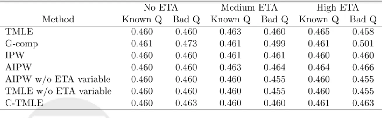
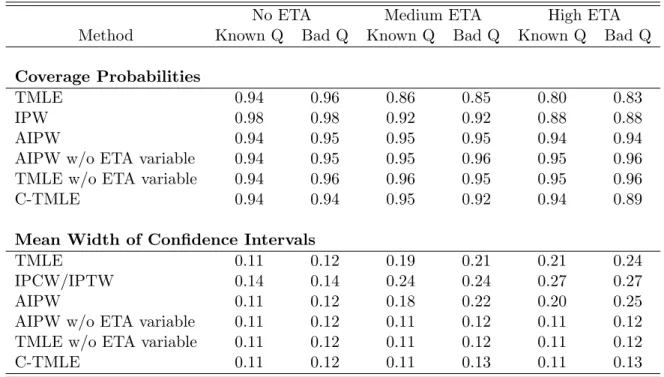
Simulation Study Results: Estimates
Tables 4 through 6 display the simulation results for the scenarios where the variable causing identifiability concerns is not a confounder. The true value of the parameter being estimated is .462. It can be seen in Table 4 that all of the methods produce unbiased estimates of the parameter of interest when the initial model for Q is specified correctly. However, when the initial model for Q is mis-specified, the G-comp estimate is biased. The IPW estimate is the same for the mis-specified and correctly specified Q since this estimate does not depend on an estimate of Q.
No ETA Medium ETA High ETA
Method Known Q Bad Q Known Q Bad Q Known Q Bad Q
TMLE 0.460 0.460 0.463 0.460 0.465 0.458
G-comp 0.461 0.473 0.461 0.499 0.461 0.501
IPW 0.460 0.460 0.461 0.461 0.460 0.460
AIPW 0.460 0.460 0.463 0.464 0.464 0.466
AIPW w/o ETA variable 0.460 0.460 0.460 0.455 0.460 0.455
TMLE w/o ETA variable 0.460 0.460 0.460 0.455 0.460 0.455
C-TMLE 0.460 0.463 0.460 0.460 0.461 0.463
Table 4: Simulation Results: Mean Of 500 Estimates (True Value Of Parameter Is .462). Variable Causing Violation In ETA Is Not A Confounder.
The fact that all of the methods produce unbiased estimates of the parameter of interest, even in the moderate sample sizes examined here, suggests that bias should not be the standard by which these methods are judged. Assessing the methods in terms of mean square error (MSE) begins to distinguish the methods from one another. Table 5 presents the root mean square error, relative efficiency (on the variance scale), and the efficiency
bound for each scenario. Again, in the no ETA scenario MSE does not distinguish the methods from one another as they all have essentially the same MSE. However, as the ETA becomes larger some of the methods begin to showcase their advantages while others lose all stability. The following observations may be made based off of Table 5:
No ETA Medium ETA High ETA
Method Known Q Bad Q Known Q Bad Q Known Q Bad Q
Efficiency Bound 0.028 0.046 0.060
Root Mean Square Error
TMLE 0.029 0.029 0.051 0.056 0.062 0.065
G-comp 0.027 0.030 0.028 0.047 0.028 0.049
IPW 0.029 0.029 0.071 0.071 0.106 0.106
AIPW 0.029 0.029 0.054 0.061 0.070 0.081
AIPW w/o ETA variable 0.029 0.029 0.030 0.031 0.029 0.031
TMLE w/o ETA variable 0.029 0.029 0.030 0.031 0.029 0.030
C-TMLE 0.028 0.031 0.029 0.037 0.029 0.040 Relative Efficiency TMLE 1.0 1.1 1.2 1.5 1.0 1.2 G-comp 0.9 1.1 0.4 1.0 0.2 0.7 IPW 1.0 1.0 2.4 2.4 3.1 3.1 AIPW 1.0 1.1 1.4 1.8 1.3 1.8
AIPW w/o ETA variable 1.0 1.1 0.4 0.5 0.2 0.3
TMLE w/o ETA variable 1.0 1.1 0.4 0.4 0.2 0.3
C-TMLE 1.0 1.2 0.4 0.7 0.2 0.4
Table 5: Simulation Results: Root Mean Square Error And Relative Efficiency. Variable Causing Violation In ETA Is Not A Confounder.
1. The IPW estimate is highly unstable with increasing ETA. In fact, the C-TMLE is six times more efficient whenQis estimated well and almost 3.5 times more efficient when Q is mis-specified in the medium ETA scenario. For the High ETA case, the C-TMLE is 15.5 times more efficient for a well estimated Q and eight times more efficient whenQis mis-specified.
2. The AIPW estimates also begin to lose stability with increasing ETA but not as much as the IPW estimates. The C-TMLE is 3.5 more times efficient than the AIPW estimate for a correctly specifiedQand 2.6 times more efficient for a mis-specifiedQ
No ETA Medium ETA High ETA
Method Known Q Bad Q Known Q Bad Q Known Q Bad Q
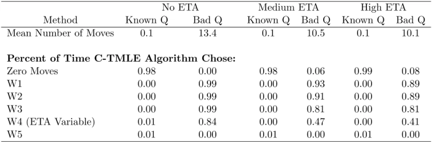
Mean Number of Moves 0.1 13.4 0.1 10.5 0.1 10.1
Percent of Time C-TMLE Algorithm Chose:
Zero Moves 0.98 0.00 0.98 0.06 0.99 0.08 W1 0.00 0.99 0.00 0.93 0.00 0.89 W2 0.00 0.99 0.00 0.91 0.00 0.89 W3 0.00 0.99 0.00 0.81 0.00 0.81 W4 (ETA Variable) 0.01 0.84 0.00 0.47 0.00 0.41 W5 0.01 0.00 0.01 0.00 0.01 0.00
Table 6: Simulation Results: Characteristics Of C-TMLE Algorithm. Variable Causing Violation In ETA Is Not A Confounder.
4.5 times more efficient for the respective ways of estimatingQ.
3. The TMLE estimate, regardless of ETA, scenario tends to have a MSE which ap-proaches the efficiency bound unlike the IPW or AIPW estimates.
4. The C-TMLE estimate is super efficient and even as the ETA violation increases, the MSE of this estimate remains close to the level it was under no ETA violation. This is true wether Q is fit well or mis-specified. The MSE is lower when Q is specified correctly; however, it still out-performs any of the other estimates in terms of efficiency whenQ is mis-specified.
Figure 2 presents two scatter plots comparing the AIPW estimates to TMLE and C-TMLE estimates in the high ETA scenario with a mis-specified Q. This is the scenario for which all estimates have the greatest difficulty in producing quality estimates (i.e. the scenario with the highest mean square error for all methods). The horizontal and vertical solid lines are the true value of the parameter being estimated, or 46.2 percent. Thus, points that are closer to the vertical black line than the horizontal black line are simulated data sets where TMLE or C-TMLE produced estimates closer to the truth than AIPW, and vice versa. These plots graphically depict the large difference in mean square error between, AIPW and TMLE, and, AIPW and C-TMLE, as seen in the last column of Table 5. In fact, the AIPW estimates range from 17.5 to 103 percent, the TMLE estimates range from 30.3 to 63.8 percent, and the C-TMLE estimates range from 35.6 to 59.2 percent. Thus, it becomes immediately clear that the AIPW does not respect the global restraints of the model by producing an estimate which is not a probability (One of the estimates is greater than 100 percent). In addition, the AIPW estimate is an empirical mean of an unbounded function of the data (Equation 11) and thus when the estimates ofg0 are close
to zero the contribution from one observation may be too large or even infinite. Whereas, the TMLE and C-TMLE estimates are empirical means of probabilities (Equation 12). By virtue of being substitution estimators each observations contribution is bounded and may be no larger than 1. The advantage of being substitution estimator is directly observed in the simulation results by the smaller mean squared error for TMLE than AIPW.
Table 6 presents some characteristics of the C-TMLE algorithm including how many, and which moves were chosen under each scenario. WhenQis specified well the C-TMLE algorithm makes very few moves and, in almost all cases, it makes zero moves leaving the intercept models forg. However, when Qis mis-specified the C-TMLE algorithm chooses more moves and attempts to adjust ing for the variables that were not adjusted for in the initial estimate ofQ. Also, the algorithm resists choosing the region of the variable which causes the ETA violations illustrated by the fact thatW4 is selected less and less as ETA increases.
Tables 7-9 display the results of the high ETA scenario, whereW1, a confounder, is the variable causing identifiability problems. The “No ETA” columns are the same as before. Table 7 displays the mean estimates for this scenario. As before whenQis specified well, all of the estimates are unbiased. However, when Q is mis-specified while the TMLE, IPW, and AIPW remain unbiased, the G-comp estimate is highly biased and the C-TMLE is slightly biased. The bias in the C-TMLE is due to the fact that it is not fully adjusting forW1 when regions of that variable contribute to non-identifiability of the parameter of interest. This bias is compensated for by the fact that the C-TMLE does as well as any of the other methods in terms of mean square error. Furthermore, the AIPW estimate does twice as bad as the C-TMLE in terms of mean square error as seen in Table 8. Though the IPW estimate is behaving reasonably in terms of bias and MSE in this simulation, its potential to provide highly unstable estimates was displayed above.
No ETA High ETA
Method Known Q Bad Q Known Q Bad Q
TMLE 0.460 0.460 0.468 0.459
G-comp 0.461 0.473 0.462 0.552
IPW 0.460 0.460 0.461 0.461
AIPW 0.460 0.460 0.462 0.466
AIPW w/o ETA variable 0.460 0.460 0.462 0.533
TMLE w/o ETA variable 0.460 0.460 0.462 0.533
C-TMLE 0.460 0.463 0.462 0.482
Table 7: Simulation Results: Mean Of 500 Estimates (True Value Of Parameter Is .462). Variable Causing Violation In ETA Is A Confounder.
No ETA High ETA
Method Known Q Bad Q Known Q Bad Q
Efficiency Bound 0.028 0.054
Root Mean Square Error
TMLE 0.029 0.029 0.053 0.050
G-comp 0.027 0.030 0.029 0.094
IPW 0.029 0.029 0.058 0.058
AIPW 0.029 0.029 0.052 0.077
AIPW w/o ETA variable 0.029 0.029 0.032 0.076
TMLE w/o ETA variable 0.029 0.029 0.031 0.076
C-TMLE 0.028 0.031 0.031 0.055 Relative Efficiency TMLE 1.0 1.1 1.0 0.9 G-comp 0.9 1.1 0.3 3.0 IPW 1.0 1.0 1.2 1.2 AIPW 1.0 1.1 0.9 2.0
AIPW w/o ETA variable 1.0 1.1 0.3 2.0
TMLE w/o ETA variable 1.0 1.1 0.3 2.0
C-TMLE 1.0 1.2 0.3 1.1
Table 8: Simulation Results: Mean Squared Error. Variable Causing Violation In ETA Is A Confounder.
correctly very few moves are made and when it is mis-specified the algorithm adjusts by choosing a fuller model forg. As expected, that the C-TMLE algorithm is having a harder time choosing what variables to adjust for now that the ETA variable is a confounder. This can be seen by the fact that the algorithm continues to adjust for W1 more often then it did for W4 in table 6. The algorithm uses the penalized loss function to weigh whether it is better to adjust for a variable which is associated with the outcome or remove it since it causes identifiability problems. In this case, the algorithm has chosen to adjust for at least some region of the variable a large percentage of the time. Had the algorithm decided to remove the variable completely from the adjustments, the estimates would be even more biased, and the MSE would be very large like the values seen for the TMLE w/o ETA variable estimate. This difference in MSE illustrates the value of generating binary variables and then running the C-TMLE algorithm on those as opposed to on the entire variable.