Deep learning and density-functional theory

(1)

UC Merced Previously Published Works

Title

Deep learning and density-functional theory

Permalink

https://escholarship.org/uc/item/1m90x23m

Journal

Physical Review A, 100(2)

ISSN

2469-9926

Authors

Ryczko, Kevin

Strubbe, David A

Tamblyn, Isaac

Publication Date

2019-08-21

DOI

10.1103/physreva.100.022512

Peer reviewed

eScholarship.org

Powered by the California Digital Library

(2)

Kevin Ryczko∗

Department of Physics, University of Ottawa David Strubbe

Department of Physics, University of California, Merced

Isaac Tamblyn†

National Research Council of Canada and Department of Physics, University of Ottawa

(Dated: June 12, 2019)

We show that deep neural networks can be integrated into, or fully replace, the Kohn-Sham den-sity functional theory scheme for multi-electron systems in simple harmonic oscillator and random external potentials with no feature engineering. We first show that self-consistent charge densities calculated with different exchange-correlation functionals can be used as input to an extensive deep neural network to make predictions for correlation, exchange, external, kinetic and total energies simultaneously. Additionally, we show that one can also make all of the same predictions with the external potential rather than the self-consistent charge density, which allows one to circumvent the Kohn-Sham scheme altogether. We then show that a self-consistent charge density found from a non-local exchange-correlation functional can be used to make energy predictions for a semi-local exchange-correlation functional. Lastly, we use a deep convolutional inverse graphics network to predict the charge density given an external potential for different exchange-correlation functionals and asses the viability of the predicted charge densities. This work shows that extensive deep neural networks are generalizable and transferable given the variability of the potentials (maximum total

energy range≈100 Ha), because they require no feature engineering, and because they can scale to

an arbitrary system size with anO(N) computational cost.

I. INTRODUCTION

Kohn-Sham (KS) density functional theory (DFT)[3] is the standard theoretical tool to study nanoscale sys-tems. Despite its success, DFT calculations for atomistic systems containing tens of thousands to millions of atoms are exceptionally demanding from a computational per-spective and are rare in the literature. Machine learning techniques can replace conventional DFT calculations to overcome this computational barrier. Machine learning models are ideal because they rival the accuracy of the method they are trained on, but can be less demand-ing to evaluate from a computational standpoint. There have been many reports where artificial neural networks (ANNs) have been used to represent potential energy sur-faces to accelerate electronic structure calculations [4– 11]. These reports focus on feature engineering or defin-ing some abstract representation of atomistic systems al-lowing one to use an ANN. Instead, we focus our review on reports that avoid feature engineering and utilize the electron density in conjunction with machine learning. More specifically, machine learning has become a popu-lar choice to represent energy functionals in DFT [12– 16], or to completely circumvent the KS scheme [17, 18]. In deep learning, the machine learning model learns the hierarchical features during training rather than

input-∗_{[email protected]}

†_{[email protected]}

ing abstract representations. Due to the large number of tuneable parameters in deep neural networks (DNNs) that may include a variety of layers (i.e. convolutional, fully connected, max pooling, etc.), there must be thou-sands (if not hundreds of thouthou-sands) of training exam-ples to find a stable minima with an acceptable accuracy. Generating these training examples is a computationally expensive task, but a trained DNN can evaluate a given quantity at a fraction of a cost compared to the original method.

An alternative, novel approach that has been taken

recently by Brockherde et al. [17] is to focus more on

uniformly sampling the space that a machine learning model will eventually predict and to use traditional ma-chine learning with far fewer tuneable parameters. This approach was successful in predicting KS-DFT total en-ergies and charge densities in one dimension (1D) for random Gaussian potentials and for small molecules in three dimensions (3D). Due to the use of Kernel Ridge Regression (KRR), they were able to achieve an accept-able accuracy with a relatively small number of training examples. Unfortunately, KRR is known to have poor scaling with respect to the number of training examples, making it difficult to train with a large (and more diverse) set of training examples.

In KS-DFT, one of the contributions to the total en-ergy is the non-interacting kinetic enen-ergy. Before the KS scheme was realized, Hohenberg and Kohn [19] pos-tulated the formalism for an interacting kinetic energy functional of the density. An analytic expression for the

(3)

9 >

>

=

>

;

<latexit sha1_base64="yGxevJxKhP5LWNbQkihwpR+ETP8=">AAACNnicbVBNSwMxEM367fpV9eglWARPZVcEPYpevAgVbBWaUrLpbBvMZpdkVihL/VNe/B3evHhQxKs/wWy7B78GZnh58ybJvChT0mIQPHszs3PzC4tLy/7K6tr6Rm1zq23T3AhoiVSl5ibiFpTU0EKJCm4yAzyJFFxHt2dl//oOjJWpvsJRBt2ED7SMpeDoqF7tgimIseGzCAZSF9wYPhoXZkx9ek8Z8ym9n9byMC1l+gx0v1JTZuRgiMzN9Gr1oBFMgv4FYQXqpIpmr/bE+qnIE9AoFLe2EwYZdt3FKIWCsc9yCxkXt3wAHQc1T8B2i8naY7rnmD6NU+NSI52w3ycKnlg7SiKnTDgO7e9eSf7X6+QYH3cLqbMcQYvpQ3GuKKa09JD2pQGBauQAF0a6v1Ix5IYLdE6XJoS/V/4L2geNMGiEl4f1k9PKjiWyQ3bJPgnJETkh56RJWkSQB/JMXsmb9+i9eO/ex1Q641Uz2+RHeJ9f8u6pBw==</latexit><latexit sha1_base64="yGxevJxKhP5LWNbQkihwpR+ETP8=">AAACNnicbVBNSwMxEM367fpV9eglWARPZVcEPYpevAgVbBWaUrLpbBvMZpdkVihL/VNe/B3evHhQxKs/wWy7B78GZnh58ybJvChT0mIQPHszs3PzC4tLy/7K6tr6Rm1zq23T3AhoiVSl5ibiFpTU0EKJCm4yAzyJFFxHt2dl//oOjJWpvsJRBt2ED7SMpeDoqF7tgimIseGzCAZSF9wYPhoXZkx9ek8Z8ym9n9byMC1l+gx0v1JTZuRgiMzN9Gr1oBFMgv4FYQXqpIpmr/bE+qnIE9AoFLe2EwYZdt3FKIWCsc9yCxkXt3wAHQc1T8B2i8naY7rnmD6NU+NSI52w3ycKnlg7SiKnTDgO7e9eSf7X6+QYH3cLqbMcQYvpQ3GuKKa09JD2pQGBauQAF0a6v1Ix5IYLdE6XJoS/V/4L2geNMGiEl4f1k9PKjiWyQ3bJPgnJETkh56RJWkSQB/JMXsmb9+i9eO/ex1Q641Uz2+RHeJ9f8u6pBw==</latexit><latexit sha1_base64="yGxevJxKhP5LWNbQkihwpR+ETP8=">AAACNnicbVBNSwMxEM367fpV9eglWARPZVcEPYpevAgVbBWaUrLpbBvMZpdkVihL/VNe/B3evHhQxKs/wWy7B78GZnh58ybJvChT0mIQPHszs3PzC4tLy/7K6tr6Rm1zq23T3AhoiVSl5ibiFpTU0EKJCm4yAzyJFFxHt2dl//oOjJWpvsJRBt2ED7SMpeDoqF7tgimIseGzCAZSF9wYPhoXZkx9ek8Z8ym9n9byMC1l+gx0v1JTZuRgiMzN9Gr1oBFMgv4FYQXqpIpmr/bE+qnIE9AoFLe2EwYZdt3FKIWCsc9yCxkXt3wAHQc1T8B2i8naY7rnmD6NU+NSI52w3ycKnlg7SiKnTDgO7e9eSf7X6+QYH3cLqbMcQYvpQ3GuKKa09JD2pQGBauQAF0a6v1Ix5IYLdE6XJoS/V/4L2geNMGiEl4f1k9PKjiWyQ3bJPgnJETkh56RJWkSQB/JMXsmb9+i9eO/ex1Q641Uz2+RHeJ9f8u6pBw==</latexit><latexit sha1_base64="yGxevJxKhP5LWNbQkihwpR+ETP8=">AAACNnicbVBNSwMxEM367fpV9eglWARPZVcEPYpevAgVbBWaUrLpbBvMZpdkVihL/VNe/B3evHhQxKs/wWy7B78GZnh58ybJvChT0mIQPHszs3PzC4tLy/7K6tr6Rm1zq23T3AhoiVSl5ibiFpTU0EKJCm4yAzyJFFxHt2dl//oOjJWpvsJRBt2ED7SMpeDoqF7tgimIseGzCAZSF9wYPhoXZkx9ek8Z8ym9n9byMC1l+gx0v1JTZuRgiMzN9Gr1oBFMgv4FYQXqpIpmr/bE+qnIE9AoFLe2EwYZdt3FKIWCsc9yCxkXt3wAHQc1T8B2i8naY7rnmD6NU+NSI52w3ycKnlg7SiKnTDgO7e9eSf7X6+QYH3cLqbMcQYvpQ3GuKKa09JD2pQGBauQAF0a6v1Ix5IYLdE6XJoS/V/4L2geNMGiEl4f1k9PKjiWyQ3bJPgnJETkh56RJWkSQB/JMXsmb9+i9eO/ex1Q641Uz2+RHeJ9f8u6pBw==</latexit>

External p oten tials Extensive Deep Neural Network Etotal Ekinetic Eexternal

a

b

Extensive Deep Neural Network Etotal Ekinetic Eexternal Eexchange Ecorrelation

9 >

>

=

>

;

<latexit sha1_base64="yGxevJxKhP5LWNbQkihwpR+ETP8=">AAACNnicbVBNSwMxEM367fpV9eglWARPZVcEPYpevAgVbBWaUrLpbBvMZpdkVihL/VNe/B3evHhQxKs/wWy7B78GZnh58ybJvChT0mIQPHszs3PzC4tLy/7K6tr6Rm1zq23T3AhoiVSl5ibiFpTU0EKJCm4yAzyJFFxHt2dl//oOjJWpvsJRBt2ED7SMpeDoqF7tgimIseGzCAZSF9wYPhoXZkx9ek8Z8ym9n9byMC1l+gx0v1JTZuRgiMzN9Gr1oBFMgv4FYQXqpIpmr/bE+qnIE9AoFLe2EwYZdt3FKIWCsc9yCxkXt3wAHQc1T8B2i8naY7rnmD6NU+NSI52w3ycKnlg7SiKnTDgO7e9eSf7X6+QYH3cLqbMcQYvpQ3GuKKa09JD2pQGBauQAF0a6v1Ix5IYLdE6XJoS/V/4L2geNMGiEl4f1k9PKjiWyQ3bJPgnJETkh56RJWkSQB/JMXsmb9+i9eO/ex1Q641Uz2+RHeJ9f8u6pBw==</latexit><latexit sha1_base64="yGxevJxKhP5LWNbQkihwpR+ETP8=">AAACNnicbVBNSwMxEM367fpV9eglWARPZVcEPYpevAgVbBWaUrLpbBvMZpdkVihL/VNe/B3evHhQxKs/wWy7B78GZnh58ybJvChT0mIQPHszs3PzC4tLy/7K6tr6Rm1zq23T3AhoiVSl5ibiFpTU0EKJCm4yAzyJFFxHt2dl//oOjJWpvsJRBt2ED7SMpeDoqF7tgimIseGzCAZSF9wYPhoXZkx9ek8Z8ym9n9byMC1l+gx0v1JTZuRgiMzN9Gr1oBFMgv4FYQXqpIpmr/bE+qnIE9AoFLe2EwYZdt3FKIWCsc9yCxkXt3wAHQc1T8B2i8naY7rnmD6NU+NSI52w3ycKnlg7SiKnTDgO7e9eSf7X6+QYH3cLqbMcQYvpQ3GuKKa09JD2pQGBauQAF0a6v1Ix5IYLdE6XJoS/V/4L2geNMGiEl4f1k9PKjiWyQ3bJPgnJETkh56RJWkSQB/JMXsmb9+i9eO/ex1Q641Uz2+RHeJ9f8u6pBw==</latexit><latexit sha1_base64="yGxevJxKhP5LWNbQkihwpR+ETP8=">AAACNnicbVBNSwMxEM367fpV9eglWARPZVcEPYpevAgVbBWaUrLpbBvMZpdkVihL/VNe/B3evHhQxKs/wWy7B78GZnh58ybJvChT0mIQPHszs3PzC4tLy/7K6tr6Rm1zq23T3AhoiVSl5ibiFpTU0EKJCm4yAzyJFFxHt2dl//oOjJWpvsJRBt2ED7SMpeDoqF7tgimIseGzCAZSF9wYPhoXZkx9ek8Z8ym9n9byMC1l+gx0v1JTZuRgiMzN9Gr1oBFMgv4FYQXqpIpmr/bE+qnIE9AoFLe2EwYZdt3FKIWCsc9yCxkXt3wAHQc1T8B2i8naY7rnmD6NU+NSI52w3ycKnlg7SiKnTDgO7e9eSf7X6+QYH3cLqbMcQYvpQ3GuKKa09JD2pQGBauQAF0a6v1Ix5IYLdE6XJoS/V/4L2geNMGiEl4f1k9PKjiWyQ3bJPgnJETkh56RJWkSQB/JMXsmb9+i9eO/ex1Q641Uz2+RHeJ9f8u6pBw==</latexit><latexit sha1_base64="yGxevJxKhP5LWNbQkihwpR+ETP8=">AAACNnicbVBNSwMxEM367fpV9eglWARPZVcEPYpevAgVbBWaUrLpbBvMZpdkVihL/VNe/B3evHhQxKs/wWy7B78GZnh58ybJvChT0mIQPHszs3PzC4tLy/7K6tr6Rm1zq23T3AhoiVSl5ibiFpTU0EKJCm4yAzyJFFxHt2dl//oOjJWpvsJRBt2ED7SMpeDoqF7tgimIseGzCAZSF9wYPhoXZkx9ek8Z8ym9n9byMC1l+gx0v1JTZuRgiMzN9Gr1oBFMgv4FYQXqpIpmr/bE+qnIE9AoFLe2EwYZdt3FKIWCsc9yCxkXt3wAHQc1T8B2i8naY7rnmD6NU+NSI52w3ycKnlg7SiKnTDgO7e9eSf7X6+QYH3cLqbMcQYvpQ3GuKKa09JD2pQGBauQAF0a6v1Ix5IYLdE6XJoS/V/4L2geNMGiEl4f1k9PKjiWyQ3bJPgnJETkh56RJWkSQB/JMXsmb9+i9eO/ex1Q641Uz2+RHeJ9f8u6pBw==</latexit>

Charge densities Deep Convolutional Inverse Graphics Network

c

Eexchange Ecorrelation

⇢

<latexit sha1_base64="yXjtFj01ayGEtbxyWlOC8kSd3gg=">AAAB63icbZDLSsNAFIZP6q3WW9Wlm8EiuCqJCLosunFZwdZCG8pkOmmGziXMTIQS+gpuXCji1hdy59s4abPQ1h8GPv5zDnPOH6WcGev7315lbX1jc6u6XdvZ3ds/qB8edY3KNKEdorjSvQgbypmkHcssp71UUywiTh+jyW1Rf3yi2jAlH+w0paHAY8liRrAtrIFO1LDe8Jv+XGgVghIaUKo9rH8NRopkgkpLODamH/ipDXOsLSOczmqDzNAUkwke075DiQU1YT7fdYbOnDNCsdLuSYvm7u+JHAtjpiJynQLbxCzXCvO/Wj+z8XWYM5lmlkqy+CjOOLIKFYejEdOUWD51gIlmbldEEqwxsS6emgshWD55FboXzcDx/WWjdVPGUYUTOIVzCOAKWnAHbegAgQSe4RXePOG9eO/ex6K14pUzx/BH3ucPH66ORw==</latexit><latexit sha1_base64="yXjtFj01ayGEtbxyWlOC8kSd3gg=">AAAB63icbZDLSsNAFIZP6q3WW9Wlm8EiuCqJCLosunFZwdZCG8pkOmmGziXMTIQS+gpuXCji1hdy59s4abPQ1h8GPv5zDnPOH6WcGev7315lbX1jc6u6XdvZ3ds/qB8edY3KNKEdorjSvQgbypmkHcssp71UUywiTh+jyW1Rf3yi2jAlH+w0paHAY8liRrAtrIFO1LDe8Jv+XGgVghIaUKo9rH8NRopkgkpLODamH/ipDXOsLSOczmqDzNAUkwke075DiQU1YT7fdYbOnDNCsdLuSYvm7u+JHAtjpiJynQLbxCzXCvO/Wj+z8XWYM5lmlkqy+CjOOLIKFYejEdOUWD51gIlmbldEEqwxsS6emgshWD55FboXzcDx/WWjdVPGUYUTOIVzCOAKWnAHbegAgQSe4RXePOG9eO/ex6K14pUzx/BH3ucPH66ORw==</latexit><latexit sha1_base64="yXjtFj01ayGEtbxyWlOC8kSd3gg=">AAAB63icbZDLSsNAFIZP6q3WW9Wlm8EiuCqJCLosunFZwdZCG8pkOmmGziXMTIQS+gpuXCji1hdy59s4abPQ1h8GPv5zDnPOH6WcGev7315lbX1jc6u6XdvZ3ds/qB8edY3KNKEdorjSvQgbypmkHcssp71UUywiTh+jyW1Rf3yi2jAlH+w0paHAY8liRrAtrIFO1LDe8Jv+XGgVghIaUKo9rH8NRopkgkpLODamH/ipDXOsLSOczmqDzNAUkwke075DiQU1YT7fdYbOnDNCsdLuSYvm7u+JHAtjpiJynQLbxCzXCvO/Wj+z8XWYM5lmlkqy+CjOOLIKFYejEdOUWD51gIlmbldEEqwxsS6emgshWD55FboXzcDx/WWjdVPGUYUTOIVzCOAKWnAHbegAgQSe4RXePOG9eO/ex6K14pUzx/BH3ucPH66ORw==</latexit><latexit sha1_base64="yXjtFj01ayGEtbxyWlOC8kSd3gg=">AAAB63icbZDLSsNAFIZP6q3WW9Wlm8EiuCqJCLosunFZwdZCG8pkOmmGziXMTIQS+gpuXCji1hdy59s4abPQ1h8GPv5zDnPOH6WcGev7315lbX1jc6u6XdvZ3ds/qB8edY3KNKEdorjSvQgbypmkHcssp71UUywiTh+jyW1Rf3yi2jAlH+w0paHAY8liRrAtrIFO1LDe8Jv+XGgVghIaUKo9rH8NRopkgkpLODamH/ipDXOsLSOczmqDzNAUkwke075DiQU1YT7fdYbOnDNCsdLuSYvm7u+JHAtjpiJynQLbxCzXCvO/Wj+z8XWYM5lmlkqy+CjOOLIKFYejEdOUWD51gIlmbldEEqwxsS6emgshWD55FboXzcDx/WWjdVPGUYUTOIVzCOAKWnAHbegAgQSe4RXePOG9eO/ex6K14pUzx/BH3ucPH66ORw==</latexit>

E

[⇢]

<latexit sha1_base64="FGGqrC+UXNUESPeTgbkftrpytm8=">AAAB7nicbZDLSgMxFIbP1Futt6pLN8EiuCozIuiyKILLCvYC06Fk0kwbmklCkhHK0Idw40IRtz6PO9/GtJ2Ftv4Q+PjPOeScP1acGev7315pbX1jc6u8XdnZ3ds/qB4etY3MNKEtIrnU3RgbypmgLcssp12lKU5jTjvx+HZW7zxRbZgUj3aiaJTioWAJI9g6q3MX9vRIRv1qza/7c6FVCAqoQaFmv/rVG0iSpVRYwrExYeArG+VYW0Y4nVZ6maEKkzEe0tChwCk1UT5fd4rOnDNAidTuCYvm7u+JHKfGTNLYdabYjsxybWb+Vwszm1xHORMqs1SQxUdJxpGVaHY7GjBNieUTB5ho5nZFZIQ1JtYlVHEhBMsnr0L7oh44frisNW6KOMpwAqdwDgFcQQPuoQktIDCGZ3iFN095L96797FoLXnFzDH8kff5AxMOj2I=</latexit><latexit sha1_base64="FGGqrC+UXNUESPeTgbkftrpytm8=">AAAB7nicbZDLSgMxFIbP1Futt6pLN8EiuCozIuiyKILLCvYC06Fk0kwbmklCkhHK0Idw40IRtz6PO9/GtJ2Ftv4Q+PjPOeScP1acGev7315pbX1jc6u8XdnZ3ds/qB4etY3MNKEtIrnU3RgbypmgLcssp12lKU5jTjvx+HZW7zxRbZgUj3aiaJTioWAJI9g6q3MX9vRIRv1qza/7c6FVCAqoQaFmv/rVG0iSpVRYwrExYeArG+VYW0Y4nVZ6maEKkzEe0tChwCk1UT5fd4rOnDNAidTuCYvm7u+JHKfGTNLYdabYjsxybWb+Vwszm1xHORMqs1SQxUdJxpGVaHY7GjBNieUTB5ho5nZFZIQ1JtYlVHEhBMsnr0L7oh44frisNW6KOMpwAqdwDgFcQQPuoQktIDCGZ3iFN095L96797FoLXnFzDH8kff5AxMOj2I=</latexit><latexit sha1_base64="FGGqrC+UXNUESPeTgbkftrpytm8=">AAAB7nicbZDLSgMxFIbP1Futt6pLN8EiuCozIuiyKILLCvYC06Fk0kwbmklCkhHK0Idw40IRtz6PO9/GtJ2Ftv4Q+PjPOeScP1acGev7315pbX1jc6u8XdnZ3ds/qB4etY3MNKEtIrnU3RgbypmgLcssp12lKU5jTjvx+HZW7zxRbZgUj3aiaJTioWAJI9g6q3MX9vRIRv1qza/7c6FVCAqoQaFmv/rVG0iSpVRYwrExYeArG+VYW0Y4nVZ6maEKkzEe0tChwCk1UT5fd4rOnDNAidTuCYvm7u+JHKfGTNLYdabYjsxybWb+Vwszm1xHORMqs1SQxUdJxpGVaHY7GjBNieUTB5ho5nZFZIQ1JtYlVHEhBMsnr0L7oh44frisNW6KOMpwAqdwDgFcQQPuoQktIDCGZ3iFN095L96797FoLXnFzDH8kff5AxMOj2I=</latexit>

<latexit sha1_base64="FGGqrC+UXNUESPeTgbkftrpytm8=">AAAB7nicbZDLSgMxFIbP1Futt6pLN8EiuCozIuiyKILLCvYC06Fk0kwbmklCkhHK0Idw40IRtz6PO9/GtJ2Ftv4Q+PjPOeScP1acGev7315pbX1jc6u8XdnZ3ds/qB4etY3MNKEtIrnU3RgbypmgLcssp12lKU5jTjvx+HZW7zxRbZgUj3aiaJTioWAJI9g6q3MX9vRIRv1qza/7c6FVCAqoQaFmv/rVG0iSpVRYwrExYeArG+VYW0Y4nVZ6maEKkzEe0tChwCk1UT5fd4rOnDNAidTuCYvm7u+JHKfGTNLYdabYjsxybWb+Vwszm1xHORMqs1SQxUdJxpGVaHY7GjBNieUTB5ho5nZFZIQ1JtYlVHEhBMsnr0L7oh44frisNW6KOMpwAqdwDgFcQQPuoQktIDCGZ3iFN095L96797FoLXnFzDH8kff5AxMOj2I=</latexit>

V

<latexit sha1_base64="Nh6msFJ35eGvdeBG/Cwngw6uv9w=">AAAB/HicbZDLSsNAFIYn9VbrLdqlm8EiuCqJCLosunFZwV6gDWEyPWmHTiZhZiKGEF/FjQtF3Pog7nwbp20W2vrDgY//nMOc+YOEM6Ud59uqrK1vbG5Vt2s7u3v7B/bhUVfFqaTQoTGPZT8gCjgT0NFMc+gnEkgUcOgF05tZv/cAUrFY3OssAS8iY8FCRok2lm/Xu34+1PCoc1MgBeFF4dsNp+nMhVfBLaGBSrV9+2s4imkagdCUE6UGrpNoLydSM8qhqA1TBQmhUzKGgUFBIlBePj++wKfGGeEwlqaExnP390ZOIqWyKDCTEdETtdybmf/1BqkOr7yciSTVIOjioTDlWMd4lgQeMQlU88wAoZKZWzGdEEmoyUHVTAju8pdXoXvedA3fXTRa12UcVXSMTtAZctElaqFb1EYdRFGGntErerOerBfr3fpYjFascqeO/sj6/AHoXpWS</latexit><latexit sha1_base64="Nh6msFJ35eGvdeBG/Cwngw6uv9w=">AAAB/HicbZDLSsNAFIYn9VbrLdqlm8EiuCqJCLosunFZwV6gDWEyPWmHTiZhZiKGEF/FjQtF3Pog7nwbp20W2vrDgY//nMOc+YOEM6Ud59uqrK1vbG5Vt2s7u3v7B/bhUVfFqaTQoTGPZT8gCjgT0NFMc+gnEkgUcOgF05tZv/cAUrFY3OssAS8iY8FCRok2lm/Xu34+1PCoc1MgBeFF4dsNp+nMhVfBLaGBSrV9+2s4imkagdCUE6UGrpNoLydSM8qhqA1TBQmhUzKGgUFBIlBePj++wKfGGeEwlqaExnP390ZOIqWyKDCTEdETtdybmf/1BqkOr7yciSTVIOjioTDlWMd4lgQeMQlU88wAoZKZWzGdEEmoyUHVTAju8pdXoXvedA3fXTRa12UcVXSMTtAZctElaqFb1EYdRFGGntErerOerBfr3fpYjFascqeO/sj6/AHoXpWS</latexit><latexit sha1_base64="Nh6msFJ35eGvdeBG/Cwngw6uv9w=">AAAB/HicbZDLSsNAFIYn9VbrLdqlm8EiuCqJCLosunFZwV6gDWEyPWmHTiZhZiKGEF/FjQtF3Pog7nwbp20W2vrDgY//nMOc+YOEM6Ud59uqrK1vbG5Vt2s7u3v7B/bhUVfFqaTQoTGPZT8gCjgT0NFMc+gnEkgUcOgF05tZv/cAUrFY3OssAS8iY8FCRok2lm/Xu34+1PCoc1MgBeFF4dsNp+nMhVfBLaGBSrV9+2s4imkagdCUE6UGrpNoLydSM8qhqA1TBQmhUzKGgUFBIlBePj++wKfGGeEwlqaExnP390ZOIqWyKDCTEdETtdybmf/1BqkOr7yciSTVIOjioTDlWMd4lgQeMQlU88wAoZKZWzGdEEmoyUHVTAju8pdXoXvedA3fXTRa12UcVXSMTtAZctElaqFb1EYdRFGGntErerOerBfr3fpYjFascqeO/sj6/AHoXpWS</latexit><latexit sha1_base64="Nh6msFJ35eGvdeBG/Cwngw6uv9w=">AAAB/HicbZDLSsNAFIYn9VbrLdqlm8EiuCqJCLosunFZwV6gDWEyPWmHTiZhZiKGEF/FjQtF3Pog7nwbp20W2vrDgY//nMOc+YOEM6Ud59uqrK1vbG5Vt2s7u3v7B/bhUVfFqaTQoTGPZT8gCjgT0NFMc+gnEkgUcOgF05tZv/cAUrFY3OssAS8iY8FCRok2lm/Xu34+1PCoc1MgBeFF4dsNp+nMhVfBLaGBSrV9+2s4imkagdCUE6UGrpNoLydSM8qhqA1TBQmhUzKGgUFBIlBePj++wKfGGeEwlqaExnP390ZOIqWyKDCTEdETtdybmf/1BqkOr7yciSTVIOjioTDlWMd4lgQeMQlU88wAoZKZWzGdEEmoyUHVTAju8pdXoXvedA3fXTRa12UcVXSMTtAZctElaqFb1EYdRFGGntErerOerBfr3fpYjFascqeO/sj6/AHoXpWS</latexit> external

E

<latexit sha1_base64="Wrb43V9n9rHg+tOIp/pDYoWtqbs=">AAAB6HicbZBNS8NAEIYn9avWr6pHL4tF8FQSEfRYFMFjC/YD2lA220m7drMJuxuhhP4CLx4U8epP8ua/cdvmoK0vLDy8M8POvEEiuDau++0U1tY3NreK26Wd3b39g/LhUUvHqWLYZLGIVSegGgWX2DTcCOwkCmkUCGwH49tZvf2ESvNYPphJgn5Eh5KHnFFjrcZdv1xxq+5cZBW8HCqQq94vf/UGMUsjlIYJqnXXcxPjZ1QZzgROS71UY0LZmA6xa1HSCLWfzRedkjPrDEgYK/ukIXP390RGI60nUWA7I2pGerk2M/+rdVMTXvsZl0lqULLFR2EqiInJ7Goy4AqZERMLlCludyVsRBVlxmZTsiF4yyevQuui6lluXFZqN3kcRTiBUzgHD66gBvdQhyYwQHiGV3hzHp0X5935WLQWnHzmGP7I+fwBmO+MyQ==</latexit> <latexit sha1_base64="Wrb43V9n9rHg+tOIp/pDYoWtqbs=">AAAB6HicbZBNS8NAEIYn9avWr6pHL4tF8FQSEfRYFMFjC/YD2lA220m7drMJuxuhhP4CLx4U8epP8ua/cdvmoK0vLDy8M8POvEEiuDau++0U1tY3NreK26Wd3b39g/LhUUvHqWLYZLGIVSegGgWX2DTcCOwkCmkUCGwH49tZvf2ESvNYPphJgn5Eh5KHnFFjrcZdv1xxq+5cZBW8HCqQq94vf/UGMUsjlIYJqnXXcxPjZ1QZzgROS71UY0LZmA6xa1HSCLWfzRedkjPrDEgYK/ukIXP390RGI60nUWA7I2pGerk2M/+rdVMTXvsZl0lqULLFR2EqiInJ7Goy4AqZERMLlCludyVsRBVlxmZTsiF4yyevQuui6lluXFZqN3kcRTiBUzgHD66gBvdQhyYwQHiGV3hzHp0X5935WLQWnHzmGP7I+fwBmO+MyQ==</latexit> <latexit sha1_base64="Wrb43V9n9rHg+tOIp/pDYoWtqbs=">AAAB6HicbZBNS8NAEIYn9avWr6pHL4tF8FQSEfRYFMFjC/YD2lA220m7drMJuxuhhP4CLx4U8epP8ua/cdvmoK0vLDy8M8POvEEiuDau++0U1tY3NreK26Wd3b39g/LhUUvHqWLYZLGIVSegGgWX2DTcCOwkCmkUCGwH49tZvf2ESvNYPphJgn5Eh5KHnFFjrcZdv1xxq+5cZBW8HCqQq94vf/UGMUsjlIYJqnXXcxPjZ1QZzgROS71UY0LZmA6xa1HSCLWfzRedkjPrDEgYK/ukIXP390RGI60nUWA7I2pGerk2M/+rdVMTXvsZl0lqULLFR2EqiInJ7Goy4AqZERMLlCludyVsRBVlxmZTsiF4yyevQuui6lluXFZqN3kcRTiBUzgHD66gBvdQhyYwQHiGV3hzHp0X5935WLQWnHzmGP7I+fwBmO+MyQ==</latexit> <latexit sha1_base64="Wrb43V9n9rHg+tOIp/pDYoWtqbs=">AAAB6HicbZBNS8NAEIYn9avWr6pHL4tF8FQSEfRYFMFjC/YD2lA220m7drMJuxuhhP4CLx4U8epP8ua/cdvmoK0vLDy8M8POvEEiuDau++0U1tY3NreK26Wd3b39g/LhUUvHqWLYZLGIVSegGgWX2DTcCOwkCmkUCGwH49tZvf2ESvNYPphJgn5Eh5KHnFFjrcZdv1xxq+5cZBW8HCqQq94vf/UGMUsjlIYJqnXXcxPjZ1QZzgROS71UY0LZmA6xa1HSCLWfzRedkjPrDEgYK/ukIXP390RGI60nUWA7I2pGerk2M/+rdVMTXvsZl0lqULLFR2EqiInJ7Goy4AqZERMLlCludyVsRBVlxmZTsiF4yyevQuui6lluXFZqN3kcRTiBUzgHD66gBvdQhyYwQHiGV3hzHp0X5935WLQWnHzmGP7I+fwBmO+MyQ==</latexit>

V

ex ter nal <latexit sha1_base64="Nh6msFJ35eGvdeBG/Cwngw6uv9w=">AAAB/HicbZDLSsNAFIYn9VbrLdqlm8EiuCqJCLosunFZwV6gDWEyPWmHTiZhZiKGEF/FjQtF3Pog7nwbp20W2vrDgY//nMOc+YOEM6Ud59uqrK1vbG5Vt2s7u3v7B/bhUVfFqaTQoTGPZT8gCjgT0NFMc+gnEkgUcOgF05tZv/cAUrFY3OssAS8iY8FCRok2lm/Xu34+1PCoc1MgBeFF4dsNp+nMhVfBLaGBSrV9+2s4imkagdCUE6UGrpNoLydSM8qhqA1TBQmhUzKGgUFBIlBePj++wKfGGeEwlqaExnP390ZOIqWyKDCTEdETtdybmf/1BqkOr7yciSTVIOjioTDlWMd4lgQeMQlU88wAoZKZWzGdEEmoyUHVTAju8pdXoXvedA3fXTRa12UcVXSMTtAZctElaqFb1EYdRFGGntErerOerBfr3fpYjFascqeO/sj6/AHoXpWS</latexit> <latexit sha1_base64="Nh6msFJ35eGvdeBG/Cwngw6uv9w=">AAAB/HicbZDLSsNAFIYn9VbrLdqlm8EiuCqJCLosunFZwV6gDWEyPWmHTiZhZiKGEF/FjQtF3Pog7nwbp20W2vrDgY//nMOc+YOEM6Ud59uqrK1vbG5Vt2s7u3v7B/bhUVfFqaTQoTGPZT8gCjgT0NFMc+gnEkgUcOgF05tZv/cAUrFY3OssAS8iY8FCRok2lm/Xu34+1PCoc1MgBeFF4dsNp+nMhVfBLaGBSrV9+2s4imkagdCUE6UGrpNoLydSM8qhqA1TBQmhUzKGgUFBIlBePj++wKfGGeEwlqaExnP390ZOIqWyKDCTEdETtdybmf/1BqkOr7yciSTVIOjioTDlWMd4lgQeMQlU88wAoZKZWzGdEEmoyUHVTAju8pdXoXvedA3fXTRa12UcVXSMTtAZctElaqFb1EYdRFGGntErerOerBfr3fpYjFascqeO/sj6/AHoXpWS</latexit> <latexit sha1_base64="Nh6msFJ35eGvdeBG/Cwngw6uv9w=">AAAB/HicbZDLSsNAFIYn9VbrLdqlm8EiuCqJCLosunFZwV6gDWEyPWmHTiZhZiKGEF/FjQtF3Pog7nwbp20W2vrDgY//nMOc+YOEM6Ud59uqrK1vbG5Vt2s7u3v7B/bhUVfFqaTQoTGPZT8gCjgT0NFMc+gnEkgUcOgF05tZv/cAUrFY3OssAS8iY8FCRok2lm/Xu34+1PCoc1MgBeFF4dsNp+nMhVfBLaGBSrV9+2s4imkagdCUE6UGrpNoLydSM8qhqA1TBQmhUzKGgUFBIlBePj++wKfGGeEwlqaExnP390ZOIqWyKDCTEdETtdybmf/1BqkOr7yciSTVIOjioTDlWMd4lgQeMQlU88wAoZKZWzGdEEmoyUHVTAju8pdXoXvedA3fXTRa12UcVXSMTtAZctElaqFb1EYdRFGGntErerOerBfr3fpYjFascqeO/sj6/AHoXpWS</latexit> <latexit sha1_base64="Nh6msFJ35eGvdeBG/Cwngw6uv9w=">AAAB/HicbZDLSsNAFIYn9VbrLdqlm8EiuCqJCLosunFZwV6gDWEyPWmHTiZhZiKGEF/FjQtF3Pog7nwbp20W2vrDgY//nMOc+YOEM6Ud59uqrK1vbG5Vt2s7u3v7B/bhUVfFqaTQoTGPZT8gCjgT0NFMc+gnEkgUcOgF05tZv/cAUrFY3OssAS8iY8FCRok2lm/Xu34+1PCoc1MgBeFF4dsNp+nMhVfBLaGBSrV9+2s4imkagdCUE6UGrpNoLydSM8qhqA1TBQmhUzKGgUFBIlBePj++wKfGGeEwlqaExnP390ZOIqWyKDCTEdETtdybmf/1BqkOr7yciSTVIOjioTDlWMd4lgQeMQlU88wAoZKZWzGdEEmoyUHVTAju8pdXoXvedA3fXTRa12UcVXSMTtAZctElaqFb1EYdRFGGntErerOerBfr3fpYjFascqeO/sj6/AHoXpWS</latexit>

⇢

<latexit sha1_base64="yXjtFj01ayGEtbxyWlOC8kSd3gg=">AAAB63icbZDLSsNAFIZP6q3WW9Wlm8EiuCqJCLosunFZwdZCG8pkOmmGziXMTIQS+gpuXCji1hdy59s4abPQ1h8GPv5zDnPOH6WcGev7315lbX1jc6u6XdvZ3ds/qB8edY3KNKEdorjSvQgbypmkHcssp71UUywiTh+jyW1Rf3yi2jAlH+w0paHAY8liRrAtrIFO1LDe8Jv+XGgVghIaUKo9rH8NRopkgkpLODamH/ipDXOsLSOczmqDzNAUkwke075DiQU1YT7fdYbOnDNCsdLuSYvm7u+JHAtjpiJynQLbxCzXCvO/Wj+z8XWYM5lmlkqy+CjOOLIKFYejEdOUWD51gIlmbldEEqwxsS6emgshWD55FboXzcDx/WWjdVPGUYUTOIVzCOAKWnAHbegAgQSe4RXePOG9eO/ex6K14pUzx/BH3ucPH66ORw==</latexit><latexit sha1_base64="yXjtFj01ayGEtbxyWlOC8kSd3gg=">AAAB63icbZDLSsNAFIZP6q3WW9Wlm8EiuCqJCLosunFZwdZCG8pkOmmGziXMTIQS+gpuXCji1hdy59s4abPQ1h8GPv5zDnPOH6WcGev7315lbX1jc6u6XdvZ3ds/qB8edY3KNKEdorjSvQgbypmkHcssp71UUywiTh+jyW1Rf3yi2jAlH+w0paHAY8liRrAtrIFO1LDe8Jv+XGgVghIaUKo9rH8NRopkgkpLODamH/ipDXOsLSOczmqDzNAUkwke075DiQU1YT7fdYbOnDNCsdLuSYvm7u+JHAtjpiJynQLbxCzXCvO/Wj+z8XWYM5lmlkqy+CjOOLIKFYejEdOUWD51gIlmbldEEqwxsS6emgshWD55FboXzcDx/WWjdVPGUYUTOIVzCOAKWnAHbegAgQSe4RXePOG9eO/ex6K14pUzx/BH3ucPH66ORw==</latexit><latexit sha1_base64="yXjtFj01ayGEtbxyWlOC8kSd3gg=">AAAB63icbZDLSsNAFIZP6q3WW9Wlm8EiuCqJCLosunFZwdZCG8pkOmmGziXMTIQS+gpuXCji1hdy59s4abPQ1h8GPv5zDnPOH6WcGev7315lbX1jc6u6XdvZ3ds/qB8edY3KNKEdorjSvQgbypmkHcssp71UUywiTh+jyW1Rf3yi2jAlH+w0paHAY8liRrAtrIFO1LDe8Jv+XGgVghIaUKo9rH8NRopkgkpLODamH/ipDXOsLSOczmqDzNAUkwke075DiQU1YT7fdYbOnDNCsdLuSYvm7u+JHAtjpiJynQLbxCzXCvO/Wj+z8XWYM5lmlkqy+CjOOLIKFYejEdOUWD51gIlmbldEEqwxsS6emgshWD55FboXzcDx/WWjdVPGUYUTOIVzCOAKWnAHbegAgQSe4RXePOG9eO/ex6K14pUzx/BH3ucPH66ORw==</latexit><latexit sha1_base64="yXjtFj01ayGEtbxyWlOC8kSd3gg=">AAAB63icbZDLSsNAFIZP6q3WW9Wlm8EiuCqJCLosunFZwdZCG8pkOmmGziXMTIQS+gpuXCji1hdy59s4abPQ1h8GPv5zDnPOH6WcGev7315lbX1jc6u6XdvZ3ds/qB8edY3KNKEdorjSvQgbypmkHcssp71UUywiTh+jyW1Rf3yi2jAlH+w0paHAY8liRrAtrIFO1LDe8Jv+XGgVghIaUKo9rH8NRopkgkpLODamH/ipDXOsLSOczmqDzNAUkwke075DiQU1YT7fdYbOnDNCsdLuSYvm7u+JHAtjpiJynQLbxCzXCvO/Wj+z8XWYM5lmlkqy+CjOOLIKFYejEdOUWD51gIlmbldEEqwxsS6emgshWD55FboXzcDx/WWjdVPGUYUTOIVzCOAKWnAHbegAgQSe4RXePOG9eO/ex6K14pUzx/BH3ucPH66ORw==</latexit>

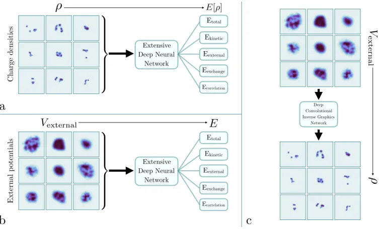
FIG. 1. A graphical representation that outlines the objectives of this report. In a. and b. we show that both charge densities and external potentials can be used as input to extensive deep neural networks (EDNNs [1]) to predict the total, kinetic, external, exchange and correlation energies. The images shown are some of the random (RND) potentials along with the self-consistent charge density for that potential. In c. we show that deep convolutional inverse graphics networks (DCIGNs [2]) can be used to map external potentials to their respective self-consistent charge densities.

exact interacting kinetic energy functional with respect to the electron density is unknown. This is one of the ma-jor downfalls of orbital-free (OF) DFT, where all energy contributions are explicitly written in terms of the elec-tron density. This shortcoming provides motivation to construct an approximate functional of the density with

a machine learning model. In a report done by Yaoet al.

[20], a convolutional neural network (CNN) was used to represent the kinetic energy functional in the OF-DFT total energy expression for various hydrocarbons. Their data generation process consisted of performing KS-DFT and collecting the charge density along with the KS non-interacting kinetic energy. The charge density was then used as input to the CNN with the KS non-interacting kinetic energy as the label. With this representation they were able to successfully reproduce potential energy sur-faces when compared to the true KS potential energy

surfaces. In another report by Snyder et al. [15], they

were able to use a machine learning model to make kinetic energy predictions given a charge density for a diatomic molecule. Using their framework, they were able to ac-curately dissociate the diatomic molecule, and compute

forces suggesting thatab initiomolecular dynamics could

eventually be done via machine learning methods.

When representing the kinetic energy with a machine learning model in the OF scheme, one then becomes con-cerned with calculating the functional derivative of the machine learning model with respect to the density. In a

report from Liet al. [14], they showed there is a

trade-off between accuracy and numerical noise to when taking the functional derivative of a machine learning model.

Brockherde et al. [17] avoided this issue by training a

machine learning model to learn the mapping between the potential and the electron density, avoiding the func-tional derivative.

In another recent report by Kolb et al. [16], a

soft-ware package was developed to combine artificial neu-ral networks with electronic structure calculations and molecular dynamics engines. Using their newly devel-oped software, they were able to show that artificial neu-ral networks can be used to make predictions with the electronic charge density as input and various energies as output. Specifically, they were able to predict energies and band gaps calculated at a higher level of theory from charge densities calculated at a lower level of theory. This approach is very advantageous as high level theory

cal-culations (i.e. G0W0[21]) become quite computationally

(4)

Although significant progress has been made incorpo-rating machine learning and deep learning to a variety of electronic structure problems, most do not have the abil-ity to properly handle extensive properties. In some of our past work, we introduced extensive DNNs (EDNNs) [1] to intrinsically learn extensive properties. This means that when the DNN learns the fundamental screening length scale it can then easily scale up to massive systems in a trivially parallel manner. EDNNs work by first di-viding up an image into fragments which are called focus regions. These fragments are then padded with context regions. The context regions may also respect periodic boundary conditions. Each of these fragments can then be simultaneously passed into machine learning models that share weights. It should be noted here that any machine learning method that uses back propagation to minimize the loss function can be used. Finally, the out-puts of the machine learning models are then summed yielding the final prediction from the EDNN.

In this report, we show that EDNNs have the capa-bility to learn energy and charge density mappings that could replace some, if not all, calculations in KS-DFT scheme. We push the frontier of what EDNNs can learn from charge densities and external potentials by calcu-lating the self-consistent charge densities in external po-tentials with extreme variabilities. In previous reports that focus on small molecules [7, 16, 17, 20], the self-consistent charge densities generated from molecular dy-namics are similar and have small energy ranges (i.e.

≈31.8 mHa [17]). We avoid small molecules (where the

charge density would be localized in space), and truly challenge the ability of EDNNs to make accurate predic-tions across a variety of electronic environments. Quan-titatively speaking the energy range of our 10 electron calculations with our random (RND) external potentials

is _≈100 Ha. This report is outlined as follows: In

Sec-tion II, we describe our data generaSec-tion process, as well as the DNN topologies and hyper-parameter selections. In Subsection III A, we show that DNNs have the capability to act as density functionals and can accurately predict the exchange, correlation, external, kinetic, and total

en-ergiessimultaneously(Subsection III A 1). We also show

that EDNNs can also circumvent the KS scheme (Subsec-tion III A 2) by mapping the external potential to all of the aforementioned energies simultaneously. Addition-ally, we show that EDNNs can be used in a somewhat “perturbative” manner, where we predict energies com-puted with semi-local or non-local exchange-correlation functionals from non-local electron densities. In Sub-section III B, we show that deep convolutional inverse graphics networks (DCIGNs) can also map the external potential to the electron density, and assess the viability of the predicted electron density. Lastly, in Section IV, we summarize our results and consider future work that could be done with our new framework. The outline of this manuscript can be seen graphically in Figure 1.

II. METHODS

We investigate two-dimensional (2D) electron gases within the KS-DFT framework [3] for two external poten-tials: simple harmonic oscillator (SHO) and RND. These external potentials have been used in a previous study [22] for direct diagonalization, one-electron calculations. In the KS-DFT framework, one minimizes the total en-ergy functional

E[ρ] =T[ρ] +Eext[ρ] +EHartree[ρ] +EXC[ρ] (1)

which leads to the expression

E[ρ(r)] = 2 N/2 X i i− 1 2 Z Z drdr0 ρ(r)ρ(r 0₎ |r₋r0_| +EXC[ρ]− Z drµxc(ρ(r))ρ(r). (2)

In Equation 1, T is the non-interacting kinetic energy,

Eextis the energy due to the interaction of the electrons

with the external potential,EHartree is the electrostatic

energy describing the electron-electron interactions,EXC

is the exchange-correlation energy, andµxc(ρ(r)) is the

same as defined in [3].

Using EDNNs, we investigate the feasibility of learning the total energy as well as the individual contributions to the total energy. We therefore have trained models to predict the total, non-interacting kinetic, external, ex-change, and correlation energies. The external potentials chosen for this report, as mentioned previously, are SHO and RND potentials in 2D. The SHO potentials take the form Vext({xi}) = 1 2 D X i ki(xi−x0i) 2 ₍₃₎

where D is the dimension, ki =mωi2 is the spring

con-stant, and x0i is the shift of the potential in a given

coordinate. For the RND potentials we follow the work

of Mills et al. [22] when generating the potentials on

a grid. We refer the reader to the original manuscript [22] for more information on the RND potential gener-ation. To briefly summarize the process, the first step consists of generating a random binary image of 0’s and 1’s and then applying a gaussian filter. The second step consists of generating a mask that is constructed with a random convex hull and an additional gaussian blur. The mask is then applied onto the image yielding the final result. The larger energy scale of the RND exter-nal potentials can be attributed to the length scales of the RND external potentials. The average Gaussian

ker-nel sizes in the external potential generation is_∼3 Bohr,

whereas the average length scale of the SHO external

po-tentials is∼12 Bohr. Assuming that the energy scales as

E ∼1/r2_{, the energy scale of the RND external}

poten-tials is 16 times larger than the SHO external potential energy scale on average. To create datasets large enough

(5)

x[˚A] 20 10 0 10 20 y[˚A]0 10 ₂₀ 10 20 Electron densit y [ ˚A 2 ] 0.0 0.1 0.2 0.3 0.4 0.5 0.6 0.7 0.8 x[˚A] 20 10 0 10 20 y[˚A]0 10 ₂₀ 10 20 Electron densit y [ ˚A 2 ] 0.0 0.1 0.2 0.3 0.4 x[˚A] 20 10 0 10 20 y[˚A]0 10 ₂₀ 10 20 Electron densit y [ ˚A 2 ] 0.00 0.05 0.10 0.15 0.20 0.25 0.30 0.35 0.40 x[˚A] 20 10 0 10 20 y[˚A]0 10 ₂₀ 10 20 Electron densit y [ ˚A 2 ] 0.000 0.025 0.050 0.075 0.100 0.125 0.150 0.175 0.200

1 electron 2 electrons 3 electrons 10 electrons

x [a0] y [a0] y [a0] x [a0] y [a0] x [a0] y [a0] x [a0] Electron densit y [ a0 -2]

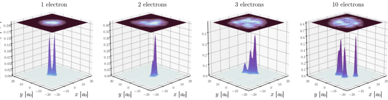
FIG. 2. Computed charge densities (3D surfaces) and random external potential energy surfaces (2D surfaces) for typical configurations of systems with 1, 2, 3, and 10 electrons.

to use DNNs, we chose to randomly sample ki and x0i

such that 0.01 _≤ ki ≤ 0.16 Ha/a20 (Hartree per Bohr2)

and ₋8.0 _≤ x0i ≤ 8.0 a0. With a given selection of

these variables, the external potential was then

evalu-ated on a 40×40a0 space with a 256×256 grid point

mesh. We then chose to place either N =1, 2, 3, or 10

electrons in the 2D space. For each choice of the num-ber of electrons, we generate an external potential, and then perform three DFT calculations, each with differ-ent exchange-correlation functionals. We used the local density approximation (LDA) exchange-correlation func-tional [23, 24], the Perdew-Burke-Ernzerhof (PBE) [25] functional for exchange and the LDA correlation func-tional, and the meta-generalized gradient approximation

(MGGA) exchange functional from Pittaliset al. [26] and

the LDA correlation functional. Here, we do not take the orbitals or charge densities from the LDA calculations to calculate energies at the PBE or MGGA level. All of the energies for each functional are calculated independently. All of the calculations were carried in real space with the Octopus code [27–29]. For testing, we set aside 10% of each data set. This made for 90,000 training configura-tions and 10,000 testing configuraconfigura-tions for each case of potential, number of electrons, and exchange-correlation functional. Note that the number of electrons and the type of external potential uniquely defines a dataset. Therefore, the 10% set aside for testing includes 10,000 external potentials and 30,000 charge densities (10,000 for each exchange-correlation functional choice). In addi-tion, the labels were normalized independently such that each of the components had a range from zero to one. The calculations are summarized in Table I of Appendix

A. All data used in this report is available online (http:

//clean.energyscience.ca/datasets) along with the

code (https://github.com/kryczko/ednn) to allow for

future development of featureless deep learning based functionals.

When constructing the EDNNs, we used a mixture of Tensorflow [30] and TFLearn [31] in Python. For the net-works topologies we build on our previous reports [1, 18] and use EDNNs where each tile of the EDNN has the same in-tile CNN used previously for predicting KS-DFT

total energies of 2D hexagonal sheets [18]. For clarity, the in-tile CNN consisted of 2 reducing convolutional layers with kernel sizes of 3, 6 non-reducing convolutional lay-ers with kernel sizes of 4, 1 reducing convolutional layer with a kernel size of 3, 4 non-reducing convolutional lay-ers with kernel sizes of 3, a fully connected layer with 1024 neurons, and a final fully connected layer with one neuron. All of the activations used were rectified lin-ear units. We emphasize that in our approach, we do not do any sort of feature engineering, like past reports that use ANNs [4–9, 16]. The convolutional layers in the EDNNs identify relevant features during the training process. When utilizing an EDNN, one must declare the focus and context regions which is used to “tile” up the image into fragments. To find the ideal focus and con-text regions, we started by training the EDNNs on the 2D charge density to total energy mapping as well as the 2D external potential to total energy mapping for the 1, 2, 3, and 10 electron systems for calculations done with the LDA exchange-correlation functional and the SHO external potential. We chose a variety of focus and con-text sizes, and found that the optimal focus and concon-text sizes are 128 pixels for the focus size, and 32 pixels for the context size. Our decision was based on a balance between accuracy and computation time. A larger focus size lowers the computation time, and a larger context size yields larger images, resulting in more neurons in the EDNNs thereby improving the accuracy of the model. For a focus of 128 pixels, we found that the accuracies were very similar for various context sizes and the choice of 32 pixels was almost arbitrary. This hyperparameter search was the most computationally demanding task for this work due to the number of models that had to be

trained. While training, we used a learning rate of 10−4

for 500 epochs when using the charge densities as input

and a learning rate of 10−5_{for 500 epochs when using the}

external potentials as input. In both cases, we further re-duced the learning rates by a factor of 10 and trained for an additional 100 epochs. For clarity, an epoch is defined to be when the weights of the network have been updated for the entire training dataset once.

(6)

0.5 0.0 0.5 0.5 0.0 0.5 0.5 0.0 0.5 2 0 2 0.5 0.0 0.5 0 50 2 0 2 0 50 True [Ha] T rue -predicted [mHa Bohr 2 e 1 ]

Exchange-Correlation Kinetic External

True [Ha]

T

rue - Predicted [mHa /

a0 2/e ] LD A PBE MGGA MGGA → LDA PBE → LDA PBE →

LDA LDA→MGGA

10e - Charge density

1e - Charge density 1e - Potential 10e - Potential

a b c d

e f g h

i j k l

m n o p

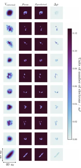
FIG. 3. True minus predicted (in mHa /a2

0 / electron) versus true (Ha) for various models with the RND potentials. Plots

a-d are models trained with the LDA exchange-correlation functional, e-f with the PBE exchange-correlation functional, and i-l with the MGGA exchange-correlation functional. First column (a, e, i) is for 1 electron models where the charge densities were used as input. Second column (b, f, j) is for 10 electron models where the charge densities were used as input. Third column (c, g, k) is for 1 electron models where the external potentials were used as input. Fourth column (d, h, l) is for 10 electrons models where the external potentials were used as input. The bottom row (m-p) is for models where LDA charge densities were used as input, and the labels were either PBE energies (m, n) or MGGA energies (o, p). Plots m, o are for the 1 electron systems, and n, p for the 10 electron systems. It should be noted that one model is predicting the correlation, exchange, external, kinetic, and total energies. We have combined the exchange-correlation error and omitted the total energy error for clarity.

III. RESULTS

A. Energy predictions

1. EDNNs as a functional

Firstly, we show that EDNNs can be used as an energy functional for correlation, exchange, external, kinetic and total energies. For the LDA, PBE, and MGGA function-als discussed in Section II, we used the computed self-consistent charge densities as input to an EDNN and were able to successfully predict the correlation, exchange, ex-ternal and total energies simultaneously for both SHO and RND external potentials. Starting with the models where the SHO external potentials were used in the DFT calculations, we found that the mean absolute errors for each particular case are less than 1.5 mHa. These can be seen in Table II of Appendix B. In Figure 3, we show

pre-dicted minus true versus true for the one and ten electron models with the different exchange-correlation function-als when the RND external potentifunction-als were used in the DFT calculations. In this Figure, it is clear that the er-ror of the models increase with the number of electrons. This increase in error is expected due to the increase in the range of energies and can be physically attributed to the increase of interactions in the system. Looking to Table III of Appendix C we also observe that the mean absolute errors become larger as the complexity of the exchange-correlation functional increases. In addi-tion to these trends, we also notice that the energy with the largest mean absolute error comes from the external energy functional. This again can be attributed to the ranges of the various energies. The external energy has the largest range of all the energies being predicted. We also address the generalizability of the models by testing the model that was trained on 10 electron charge

(7)

den-sities calculated with the RND external potentials and the LDA functional with 10 electron charge densities cal-culated with the SHO external potentials and the LDA functional (and vice versa). We found in both cases the errors increased by several orders of magnitude. This is not surprising given the different energy ranges of the datasets. On the contrary, when examining the true ver-sus predicted plot for the model trained on the RND dataset but tested on with the SHO dataset, we found that a constant shift could simply be added to substan-tially decrease the error. We expect that this constant shift could be easily rectified if SHO training examples are included in the training process.

DFT is a more popular choice for larger systems relative to wavefunction based methods because the exchange-correlation functionals used are computation-ally inexpensive relative to methods that employ exact exchange, for example. In light of this, we have trained EDNNs to predict energies at the PBE and MGGA level given a self-consistent charge density computed with the LDA exchange-correlation functional. In Figure 3, we consider 1 and 10 electron models trained on the mapping between LDA charge densities and either PBE or MGGA energies. Similar to the results mentioned above, the mean absolute errors increase both with the number of electrons and the complexity of the exchange-correlation functional. In Table III of Appendix C, we also notice that the highest mean absolute error is for the exter-nal and total energies. This result further suggests that there is not a fundamental problem with learning the ex-ternal energy, but the larger range of energies makes it more difficult for a EDNN to handle with extreme preci-sion. In addition, since the correlation functional is the same across all of the calculations and the same testing data was used for each case of number of electrons, we can determine if the networks are learning the correla-tion energy in a similar manner. In Table III, we can see that the correlation energies have similar magnitudes of error indicating that similar correlation functional map-pings are being learned as one should expect. The suc-cess of learning the energies of a more accurate exchange-correlation functional given a less accurate charge density shows promise for other applications. A future

applica-tion could include learning a G0W0 total energy from a

DFT computed self-consistent charge density, similar to

the work that was completed by Kolbet al. [16].

A note should be made about Table III with respect to the magnitude of some of the mean absolute errors

re-ported. In comparison to the report by Millset al. [22],

some of the mean absolute errors are larger by some cases a factor of 10. In addition, the focus and context hyper-parameters were optimized for the SHO external

poten-tials. In the work of Brockherde et al. [17], they

man-aged to reach chemical accuracy using three dimensional charge densities, but the energy range of their training

set was≈40 kcal/mol (for a benzene molecule). For their

best reported model with a mean absolute error of 0.28 kcal/mol, the relative mean absolute error, that we

de-fine as the mean absolute error divided by the range of the dataset is 0.007. In our 10 electron model with the

RND external potential, our energy range was_≈100 Ha

(62750.9 kcal/mol) and the mean absolute error of the to-tal energy predictions was 78.514 mHa yielding a relative

mean absolute error of 7.85×10−4_.

2. Circumventing Kohn-Sham DFT

In addition to using EDNNs as a functional, it is ar-guably more convenient to train a EDNN to learn the mapping between the external potential and the con-tributing energies of that system. It is more convenient because it avoids calculating a self-consistent charge den-sity with the KS scheme. We have trained EDNNs to predict the exchange, correlation, external, kinetic, and total energy simultaneously using the external potential as input rather than the charge density. Again, in Fig-ure 3 we show true minus predicted versus true for the correlation, exchange, external, kinetic, total energies for the RND external potentials. Here, it is evident that the charge density is more optimal as an input to an EDNN for the 1 electron systems. There is much more spread in the distribution when using external potentials as input compared to charge densities. For 10 electrons, this is not the case. Looking to Table III of Appendix C, we can see that for 1, 2, and 3 electrons no matter what choice of exchange-correlation functional, it is less

diffi-cult to learn the mapping betweenρ→E thanV →E.

The mean absolute errors are lower for all energies. In the case of 10 electrons, the mean absolute errors in the external and total energies are lower for the models that have potentials as input. Although the errors are lower for the external and total energies, the mean absolute errors for correlation, exchange, and kinetic energies are larger. When training a model on a set of energies, there is a balance between the errors of the energies since the loss function depends on the sum over the mean squared errors between the true and predicted energies. In the case of using charge densities as input to the EDNN, we found the exchange, correlation, and kinetic energies can be predicted with much better accuracy than the exter-nal or total energies. In the case of using potentials as input to the EDNN, we found that there is more of a balance of accuracy between the different energies being predicted.

B. Image predictions with Deep Convolutional

Inverse Graphics Networks

In both KS-DFT and OF-DFT, the self-consistent charge density is the central quantity that one is inter-ested in calculating. Once one has the charge density, most other quantities can be calculated in a straightfor-ward manner. In this Subsection, we address the via-bility of using DCIGNs to map the external potential to

(8)

the self-consistent charge density in 2D for the RND po-tentials with the LDA, PBE, and MGGA exchange cor-relation functionals. DCIGNs were recently introduced in the literature [2] and have a similar topology to au-toencoders [32]. The DCIGN that we have used has 4 reducing convolutional layers, 3 non-reducing convolu-tional layers, and 4 deconvoluconvolu-tional layers such that the output image has the same dimensionality as the input image. This topology differs slightly from the original work on DCIGNs [2], where a fully connected would re-place our 3 non-reducing convolutional layers. Addition-ally, our DCIGN is deterministic. In the original work [2], random noise is introduced in the decoder to create a non-deterministic generative model. All of our convo-lutional layers use a kernel size of 3 with rectified linear

unit activations. We used a learning rate of 10−5 _while

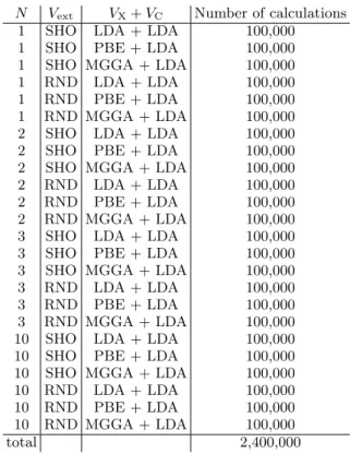
training for 500 epochs and dropped the learning rate by a factor of 10 before training for an additional 100 epochs. For this discussion we focus solely on the 10 electron cal-culations with the RND external potentials. We argue that these are the most challenging calculations to train with a DCIGN, and can therefore safely assume that the less complex calculations would be successful given the success of the most complex cases. In Figure 4, we show some of the predictions that the DCIGN made for 10 electrons calculations with the LDA exchange-correlation functional. There is a remarkable resemblance between

the true (ρtrue) and predicted (ρpredicted) charge

densi-ties. The DCIGN is capable of handling the extreme variability of the complex shapes, and is capable of han-dling the cases where the charge density is not isolated to one region of space. From a qualitative perspective, the DCIGN makes accurate predictions of the charge densi-ties given RND external potentials.

Normally, when addressing the viability of a machine learning model from a quantitative perspective one con-siders the mean absolute error on the test set. We argue

that a more rigorous test forρpredictedwould be mean

ab-solute error of the energies associated withρpredicted. We

therefore take ρpredicted and renormalize them such that

R

dr ρ(r)predicted = 10. Afterwards, we use the

renor-malizedρpredicted as input to a subset of the models

de-scribed in Subsection III A 1. We then compare the

en-ergies predicted fromρpredictedwith the true energies. In

Table III of Appendix C, we show the mean absolute errors between the true and predicted energies for the different exchange-correlation functionals. When com-paring the mean absolute errors of the predicted energies

forρpredicted with the energy predictions made from the

ρtrue, the minimal difference was seen for the correlation

energies with a value of ∼6 mHa. This was true for all

exchange-correlation functionals considered in this work. The maximal difference between the mean absolute

er-rors when comparing the energy predictions of ρpredicted

and ρtrue was the total energy which was ∼ 20 mHa.

Again, this is true for all exchange-correlation function-als considered. In addition to this metric, we function-also report

the mean absolute error for a model mapping ρpredicted

Vexternal

<latexit sha1_base64="Nh6msFJ35eGvdeBG/Cwngw6uv9w=">AAAB/HicbZDLSsNAFIYn9VbrLdqlm8EiuCqJCLosunFZwV6gDWEyPWmHTiZhZiKGEF/FjQtF3Pog7nwbp20W2vrDgY//nMOc+YOEM6Ud59uqrK1vbG5Vt2s7u3v7B/bhUVfFqaTQoTGPZT8gCjgT0NFMc+gnEkgUcOgF05tZv/cAUrFY3OssAS8iY8FCRok2lm/Xu34+1PCoc1MgBeFF4dsNp+nMhVfBLaGBSrV9+2s4imkagdCUE6UGrpNoLydSM8qhqA1TBQmhUzKGgUFBIlBePj++wKfGGeEwlqaExnP390ZOIqWyKDCTEdETtdybmf/1BqkOr7yciSTVIOjioTDlWMd4lgQeMQlU88wAoZKZWzGdEEmoyUHVTAju8pdXoXvedA3fXTRa12UcVXSMTtAZctElaqFb1EYdRFGGntErerOerBfr3fpYjFascqeO/sj6/AHoXpWS</latexit>

<latexit sha1_base64="Nh6msFJ35eGvdeBG/Cwngw6uv9w=">AAAB/HicbZDLSsNAFIYn9VbrLdqlm8EiuCqJCLosunFZwV6gDWEyPWmHTiZhZiKGEF/FjQtF3Pog7nwbp20W2vrDgY//nMOc+YOEM6Ud59uqrK1vbG5Vt2s7u3v7B/bhUVfFqaTQoTGPZT8gCjgT0NFMc+gnEkgUcOgF05tZv/cAUrFY3OssAS8iY8FCRok2lm/Xu34+1PCoc1MgBeFF4dsNp+nMhVfBLaGBSrV9+2s4imkagdCUE6UGrpNoLydSM8qhqA1TBQmhUzKGgUFBIlBePj++wKfGGeEwlqaExnP390ZOIqWyKDCTEdETtdybmf/1BqkOr7yciSTVIOjioTDlWMd4lgQeMQlU88wAoZKZWzGdEEmoyUHVTAju8pdXoXvedA3fXTRa12UcVXSMTtAZctElaqFb1EYdRFGGntErerOerBfr3fpYjFascqeO/sj6/AHoXpWS</latexit> ⇢<latexit sha1_base64="Su/+mDiOwOAj8MHJEPagHC7jpJg=">AAAB+3icbZDLSsNAFIYn9VbrLdalm2ARXJVEBF0W3bisYC/QhDCZnrRDJxdmTqQl5FXcuFDErS/izrdx2mahrT8MfPznHM6ZP0gFV2jb30ZlY3Nre6e6W9vbPzg8Mo/rXZVkkkGHJSKR/YAqEDyGDnIU0E8l0CgQ0Asmd/N67wmk4kn8iLMUvIiOYh5yRlFbvll35TjxcxdhijnKDIrCNxt2017IWgenhAYp1fbNL3eYsCyCGJmgSg0cO0UvpxI5E1DU3ExBStmEjmCgMaYRKC9f3F5Y59oZWmEi9YvRWri/J3IaKTWLAt0ZURyr1drc/K82yDC88XIepxlCzJaLwkxYmFjzIKwhl8BQzDRQJrm+1WJjKilDHVdNh+CsfnkdupdNR/PDVaN1W8ZRJafkjFwQh1yTFrknbdIhjEzJM3klb0ZhvBjvxseytWKUMyfkj4zPHzzclTQ=</latexit><latexit sha1_base64="Su/+mDiOwOAj8MHJEPagHC7jpJg=">AAAB+3icbZDLSsNAFIYn9VbrLdalm2ARXJVEBF0W3bisYC/QhDCZnrRDJxdmTqQl5FXcuFDErS/izrdx2mahrT8MfPznHM6ZP0gFV2jb30ZlY3Nre6e6W9vbPzg8Mo/rXZVkkkGHJSKR/YAqEDyGDnIU0E8l0CgQ0Asmd/N67wmk4kn8iLMUvIiOYh5yRlFbvll35TjxcxdhijnKDIrCNxt2017IWgenhAYp1fbNL3eYsCyCGJmgSg0cO0UvpxI5E1DU3ExBStmEjmCgMaYRKC9f3F5Y59oZWmEi9YvRWri/J3IaKTWLAt0ZURyr1drc/K82yDC88XIepxlCzJaLwkxYmFjzIKwhl8BQzDRQJrm+1WJjKilDHVdNh+CsfnkdupdNR/PDVaN1W8ZRJafkjFwQh1yTFrknbdIhjEzJM3klb0ZhvBjvxseytWKUMyfkj4zPHzzclTQ=</latexit><latexit sha1_base64="Su/+mDiOwOAj8MHJEPagHC7jpJg=">AAAB+3icbZDLSsNAFIYn9VbrLdalm2ARXJVEBF0W3bisYC/QhDCZnrRDJxdmTqQl5FXcuFDErS/izrdx2mahrT8MfPznHM6ZP0gFV2jb30ZlY3Nre6e6W9vbPzg8Mo/rXZVkkkGHJSKR/YAqEDyGDnIU0E8l0CgQ0Asmd/N67wmk4kn8iLMUvIiOYh5yRlFbvll35TjxcxdhijnKDIrCNxt2017IWgenhAYp1fbNL3eYsCyCGJmgSg0cO0UvpxI5E1DU3ExBStmEjmCgMaYRKC9f3F5Y59oZWmEi9YvRWri/J3IaKTWLAt0ZURyr1drc/K82yDC88XIepxlCzJaLwkxYmFjzIKwhl8BQzDRQJrm+1WJjKilDHVdNh+CsfnkdupdNR/PDVaN1W8ZRJafkjFwQh1yTFrknbdIhjEzJM3klb0ZhvBjvxseytWKUMyfkj4zPHzzclTQ=</latexit><latexit sha1_base64="Su/+mDiOwOAj8MHJEPagHC7jpJg=">AAAB+3icbZDLSsNAFIYn9VbrLdalm2ARXJVEBF0W3bisYC/QhDCZnrRDJxdmTqQl5FXcuFDErS/izrdx2mahrT8MfPznHM6ZP0gFV2jb30ZlY3Nre6e6W9vbPzg8Mo/rXZVkkkGHJSKR/YAqEDyGDnIU0E8l0CgQ0Asmd/N67wmk4kn8iLMUvIiOYh5yRlFbvll35TjxcxdhijnKDIrCNxt2017IWgenhAYp1fbNL3eYsCyCGJmgSg0cO0UvpxI5E1DU3ExBStmEjmCgMaYRKC9f3F5Y59oZWmEi9YvRWri/J3IaKTWLAt0ZURyr1drc/K82yDC88XIepxlCzJaLwkxYmFjzIKwhl8BQzDRQJrm+1WJjKilDHVdNh+CsfnkdupdNR/PDVaN1W8ZRJafkjFwQh1yTFrknbdIhjEzJM3klb0ZhvBjvxseytWKUMyfkj4zPHzzclTQ=</latexit> true ⇢<latexit sha1_base64="7cekkzT2J869qqsBZzNX5MJEC54=">AAACAHicbVDLSsNAFJ3UV62vqAsXboJFcFUSEXRZdOOygn1AE8JkctsOnTyYuRFLyMZfceNCEbd+hjv/xmmbhbYeGDiccw937glSwRXa9rdRWVldW9+obta2tnd298z9g45KMsmgzRKRyF5AFQgeQxs5CuilEmgUCOgG45up330AqXgS3+MkBS+iw5gPOKOoJd88cuUo8XMX4RFznQw5QwiLwjfrdsOewVomTknqpETLN7/cMGFZBDEyQZXqO3aKXk4lciagqLmZgpSyMR1CX9OYRqC8fHZAYZ1qJbQGidQvRmum/k7kNFJqEgV6MqI4UoveVPzP62c4uPJyHqcZQszmiwaZsDCxpm1YIZfAUEw0oUxy/VeLjaikugSparoEZ/HkZdI5bzia313Um9dlHVVyTE7IGXHIJWmSW9IibcJIQZ7JK3kznowX4934mI9WjDJzSP7A+PwBFnmXWg==</latexit><latexit sha1_base64="7cekkzT2J869qqsBZzNX5MJEC54=">AAACAHicbVDLSsNAFJ3UV62vqAsXboJFcFUSEXRZdOOygn1AE8JkctsOnTyYuRFLyMZfceNCEbd+hjv/xmmbhbYeGDiccw937glSwRXa9rdRWVldW9+obta2tnd298z9g45KMsmgzRKRyF5AFQgeQxs5CuilEmgUCOgG45up330AqXgS3+MkBS+iw5gPOKOoJd88cuUo8XMX4RFznQw5QwiLwjfrdsOewVomTknqpETLN7/cMGFZBDEyQZXqO3aKXk4lciagqLmZgpSyMR1CX9OYRqC8fHZAYZ1qJbQGidQvRmum/k7kNFJqEgV6MqI4UoveVPzP62c4uPJyHqcZQszmiwaZsDCxpm1YIZfAUEw0oUxy/VeLjaikugSparoEZ/HkZdI5bzia313Um9dlHVVyTE7IGXHIJWmSW9IibcJIQZ7JK3kznowX4934mI9WjDJzSP7A+PwBFnmXWg==</latexit><latexit sha1_base64="7cekkzT2J869qqsBZzNX5MJEC54=">AAACAHicbVDLSsNAFJ3UV62vqAsXboJFcFUSEXRZdOOygn1AE8JkctsOnTyYuRFLyMZfceNCEbd+hjv/xmmbhbYeGDiccw937glSwRXa9rdRWVldW9+obta2tnd298z9g45KMsmgzRKRyF5AFQgeQxs5CuilEmgUCOgG45up330AqXgS3+MkBS+iw5gPOKOoJd88cuUo8XMX4RFznQw5QwiLwjfrdsOewVomTknqpETLN7/cMGFZBDEyQZXqO3aKXk4lciagqLmZgpSyMR1CX9OYRqC8fHZAYZ1qJbQGidQvRmum/k7kNFJqEgV6MqI4UoveVPzP62c4uPJyHqcZQszmiwaZsDCxpm1YIZfAUEw0oUxy/VeLjaikugSparoEZ/HkZdI5bzia313Um9dlHVVyTE7IGXHIJWmSW9IibcJIQZ7JK3kznowX4934mI9WjDJzSP7A+PwBFnmXWg==</latexit><latexit sha1_base64="7cekkzT2J869qqsBZzNX5MJEC54=">AAACAHicbVDLSsNAFJ3UV62vqAsXboJFcFUSEXRZdOOygn1AE8JkctsOnTyYuRFLyMZfceNCEbd+hjv/xmmbhbYeGDiccw937glSwRXa9rdRWVldW9+obta2tnd298z9g45KMsmgzRKRyF5AFQgeQxs5CuilEmgUCOgG45up330AqXgS3+MkBS+iw5gPOKOoJd88cuUo8XMX4RFznQw5QwiLwjfrdsOewVomTknqpETLN7/cMGFZBDEyQZXqO3aKXk4lciagqLmZgpSyMR1CX9OYRqC8fHZAYZ1qJbQGidQvRmum/k7kNFJqEgV6MqI4UoveVPzP62c4uPJyHqcZQszmiwaZsDCxpm1YIZfAUEw0oUxy/VeLjaikugSparoEZ/HkZdI5bzia313Um9dlHVVyTE7IGXHIJWmSW9IibcJIQZ7JK3kznowX4934mI9WjDJzSP7A+PwBFnmXWg==</latexit>predicted ⇢

<latexit sha1_base64="wHSqg3SI7mavIJwBTvDS6SSk/D8=">AAAB8nicbZBNS8NAEIY39avWr6pHL4tF8FQSEfRY1IPHCvYDklA220m7dJMNuxOhlP4MLx4U8eqv8ea/cdvmoK0vLDy8M8POvFEmhUHX/XZKa+sbm1vl7crO7t7+QfXwqG1Urjm0uJJKdyNmQIoUWihQQjfTwJJIQica3c7qnSfQRqj0EccZhAkbpCIWnKG1/OAOJDIa6KHqVWtu3Z2LroJXQI0UavaqX0Ff8TyBFLlkxviem2E4YRoFlzCtBLmBjPERG4BvMWUJmHAyX3lKz6zTp7HS9qVI5+7viQlLjBknke1MGA7Ncm1m/lfzc4yvw4lIsxwh5YuP4lxSVHR2P+0LDRzl2ALjWthdKR8yzTjalCo2BG/55FVoX9Q9yw+XtcZNEUeZnJBTck48ckUa5J40SYtwosgzeSVvDjovzrvzsWgtOcXMMfkj5/MH1keQ8w==</latexit> <latexit sha1_base64="wHSqg3SI7mavIJwBTvDS6SSk/D8=">AAAB8nicbZBNS8NAEIY39avWr6pHL4tF8FQSEfRY1IPHCvYDklA220m7dJMNuxOhlP4MLx4U8eqv8ea/cdvmoK0vLDy8M8POvFEmhUHX/XZKa+sbm1vl7crO7t7+QfXwqG1Urjm0uJJKdyNmQIoUWihQQjfTwJJIQica3c7qnSfQRqj0EccZhAkbpCIWnKG1/OAOJDIa6KHqVWtu3Z2LroJXQI0UavaqX0Ff8TyBFLlkxviem2E4YRoFlzCtBLmBjPERG4BvMWUJmHAyX3lKz6zTp7HS9qVI5+7viQlLjBknke1MGA7Ncm1m/lfzc4yvw4lIsxwh5YuP4lxSVHR2P+0LDRzl2ALjWthdKR8yzTjalCo2BG/55FVoX9Q9yw+XtcZNEUeZnJBTck48ckUa5J40SYtwosgzeSVvDjovzrvzsWgtOcXMMfkj5/MH1keQ8w==</latexit> <latexit sha1_base64="wHSqg3SI7mavIJwBTvDS6SSk/D8=">AAAB8nicbZBNS8NAEIY39avWr6pHL4tF8FQSEfRY1IPHCvYDklA220m7dJMNuxOhlP4MLx4U8eqv8ea/cdvmoK0vLDy8M8POvFEmhUHX/XZKa+sbm1vl7crO7t7+QfXwqG1Urjm0uJJKdyNmQIoUWihQQjfTwJJIQica3c7qnSfQRqj0EccZhAkbpCIWnKG1/OAOJDIa6KHqVWtu3Z2LroJXQI0UavaqX0Ff8TyBFLlkxviem2E4YRoFlzCtBLmBjPERG4BvMWUJmHAyX3lKz6zTp7HS9qVI5+7viQlLjBknke1MGA7Ncm1m/lfzc4yvw4lIsxwh5YuP4lxSVHR2P+0LDRzl2ALjWthdKR8yzTjalCo2BG/55FVoX9Q9yw+XtcZNEUeZnJBTck48ckUa5J40SYtwosgzeSVvDjovzrvzsWgtOcXMMfkj5/MH1keQ8w==</latexit> <latexit sha1_base64="wHSqg3SI7mavIJwBTvDS6SSk/D8=">AAAB8nicbZBNS8NAEIY39avWr6pHL4tF8FQSEfRY1IPHCvYDklA220m7dJMNuxOhlP4MLx4U8eqv8ea/cdvmoK0vLDy8M8POvFEmhUHX/XZKa+sbm1vl7crO7t7+QfXwqG1Urjm0uJJKdyNmQIoUWihQQjfTwJJIQica3c7qnSfQRqj0EccZhAkbpCIWnKG1/OAOJDIa6KHqVWtu3Z2LroJXQI0UavaqX0Ff8TyBFLlkxviem2E4YRoFlzCtBLmBjPERG4BvMWUJmHAyX3lKz6zTp7HS9qVI5+7viQlLjBknke1MGA7Ncm1m/lfzc4yvw4lIsxwh5YuP4lxSVHR2P+0LDRzl2ALjWthdKR8yzTjalCo2BG/55FVoX9Q9yw+XtcZNEUeZnJBTck48ckUa5J40SYtwosgzeSVvDjovzrvzsWgtOcXMMfkj5/MH1keQ8w==</latexit> 40 a0 40 a0 0.00 0.02 0.04 0.06 0.08 0.10 0.12 Units of n um ber of electrons / a 0₂

FIG. 4. Examples of the RND potentials, true charge

densi-ties (ρtrue), predicted charge densities (ρpredicted), and

differ-ences between the true and predicted charge densities (∆ρ). The charge densities shown here were computed with the LDA

exchange-correlation functional. The colour bar is for the

charge density differences ∆ρ.

to the true energies. We find an increase in the errors in comparison to the models that map the true charge den-sities to the true energies, but the errors are comparable

to the errors when we evaluateρpredicted with the model

trained on the true charge densities. Training with the charge densities and energies as labels yields similar re-sults. We also report the density driven error (DDE)

us-ing the same definition as Brockherdeet al. [17] in Table

III. We find similar trends in the DDEs when comparing

them to the mean absolute errors ofρpredicted. In

addi-tion, to compare with Brockherdeet al. [17], our relative

(9)

IV. CONCLUSION

In conclusion, we have shown that EDNNs and DCIGNs can be used alongside, or replace conventional KS-DFT calculations. For both the RND and SHO ex-ternal potentials, EDNNs have the capability to make highly accurate energy predictions using both the charge densities and the external potentials as input for corre-lation, exchange, external, kinetic and total energy

si-multaneously (dataset is available online here: http:

//clean.energyscience.ca/datasets). In addition,

we have shown that DCIGNs have the capability to pre-dict charge densities given an external potential. Qual-itatively speaking, the predicted charge densities are re-markably similar to the true charge densities. Quantita-tively speaking, the relative mean absolute errors were

found to be smaller than previous, state-of-the-art work [17]. The results of this report show promise for future application in two regards. First, that this framework has the capability to make predictions of higher level the-ory calculations given a lower level thethe-ory charge density similar to a previous report [16]. Second, both EDNNs and DCIGNs can be used to calculate energies covering a large range of electronic environments to a high level of accuracy.

V. ACKNOWLEDGEMENTS

The authors acknowledge funding from the Natural Sciences and Engineering Research Council of Canada, and Compute Canada and SOSCIP for computational resources. The authors would also like to thank NVIDIA for a faculty hardware grant.

[1] K. Mills, K. Ryczko, I. Luchak, A. Domurad, C. Beeler, and I. Tamblyn, Chemical Science (2019).

[2] T. D. Kulkarni, W. F. Whitney, P. Kohli, and J.

Tenen-baum, inAdvances in Neural Information Processing

Sys-tems 28, edited by C. Cortes, N. D. Lawrence, D. D. Lee,

M. Sugiyama, and R. Garnett (Curran Associates, Inc., 2015) pp. 2539–2547.

[3] W. Kohn and L. J. Sham, Physical Review Letters140,

A1133 (1965).

[4] J. Behler, Physical Chemistry Chemical Physics 13,

17930 (2011).

[5] S. Lorenz, A. Gro, and M. Scheffler, Chemical Physics

Letters395, 210 (2004).

[6] C. M. Handley and P. L. A. Popelier, The Journal

of Physical Chemistry A 114, 3371 (2010), pMID:

20131763, https://doi.org/10.1021/jp9105585.

[7] R. M. Balabin and E. I. Lomakina, The

Jour-nal of Chemical Physics 131, 074104 (2009),

https://doi.org/10.1063/1.3206326.

[8] J. Behler and M. Parrinello, Physical Review Letters98,

146401 (2007).

[9] C. Xie, X. Zhu, D. R. Yarkony, and H. Guo,

The Journal of Chemical Physics 149, 144107 (2018),

https://doi.org/10.1063/1.5054310.

[10] K. Sch¨utt, P.-J. Kindermans, H. E. S. Felix, S. Chmiela,

A. Tkatchenko, and K.-R. M¨uller, inAdvances in Neural

Information Processing Systems (2017) pp. 991–1001.

[11] K. T. Sch¨utt, F. Arbabzadah, S. Chmiela, K. R. M¨uller,

and A. Tkatchenko, Nature Communications 8, 13890

(2017).

[12] J. C. Snyder, M. Rupp, K. Hansen, K.-R. M¨uller, and

K. Burke, Physical Review Letters108, 253002 (2012).

[13] L. Li, T. E. Baker, S. R. White, and K. Burke, Physical

Review B94, 245129 (2016).

[14] L. Li, J. C. Snyder, I. M. Pelaschier, J. Huang, U.-N. Niranjan, P. Duncan, M. Rupp, K.-R. M, and K. Burke,

International Journal of Quantum Chemistry 116, 819

(2016).

[15] J. C. Snyder, M. Rupp, K. Hansen, L. Blooston, K.-R.

M¨uller, and K. Burke, Journal of Chemical Physics139,

224104 (2013).

[16] B. Kolb, L. C. Lentz, and A. M. Kolpak, Scientific

Re-ports7(2017), 10.1038/s41598-017-01251-z.

[17] F. Brockherde, L. Vogt, L. Li, M. E. Tuckerman,

K. Burke, and K.-R. Muller, Nature Communications

8(2016).

[18] K. Ryczko, K. Mills, I. Luchak, C. Homenick, and

I. Tamblyn, Computational Materials Science 149, 134

(2018).

[19] P. Hohenberg and W. Kohn, Physical Review Letters 136, B864 (1964).

[20] K. Yao and J. Parkhill, Journal of Chemical Theory and

Computation12, 1139 (2016).

[21] M. S. Hybertsen and S. G. Louie, Physical Review B34,

5390 (1986).

[22] K. Mills, M. Spanner, and I. Tamblyn, Physical Review

A96, 042113 (2017).

[23] P. A. M. Dirac, Mathematical Proceedings of the

Cam-bridge Philosophical Society26, 376385 (1930).

[24] m. F. Bloch, Zeitschrift f¨ur Physik A Hadrons and Nuclei

57, 545 (1929).

[25] J. P. Perdew, K. Burke, and M. Ernzerhof, Physical

Review Letters77, 3865 (1996).

[26] S. Pittalis, E. R¨as¨anen, N. Helbig, and E. Gross, Physical

Review B76, 235314 (2007).

[27] X. Andrade, D. Strubbe, U. De Giovannini, A. H. Larsen, M. J. Oliveira, J. Alberdi-Rodriguez, A. Varas,

I. Theophilou, N. Helbig, M. J. Verstraete,et al.,

Physi-cal Chemistry ChemiPhysi-cal Physics17, 31371 (2015).

[28] X. Andrade, J. Alberdi-Rodriguez, D. A. Strubbe, M. J. Oliveira, F. Nogueira, A. Castro, J. Muguerza, A.

Arru-abarrena, S. G. Louie, A. Aspuru-Guzik,et al., Journal

of Physics: Condensed Matter24, 233202 (2012).

[29] X. Andrade and A. Aspuru-Guzik, Journal of Chemical

Theory and Computation9, 4360 (2013).

[30] M. Abadi, P. Barham, J. Chen, Z. Chen, A. Davis, J. Dean, M. Devin, S. Ghemawat, G. Irving, M. Isard,

et al., inOSDI, Vol. 16 (2016) pp. 265–283.

(10)

[32] I. Goodfellow, Y. Bengio, and A. Courville,Deep

Learn-ing (MIT Press, 2016) http://www.deeplearningbook.

org.

Appendix A: More details on the generated data

N Vext VX+VC Number of calculations

1 SHO LDA + LDA 100,000

1 SHO PBE + LDA 100,000

1 SHO MGGA + LDA 100,000

1 RND LDA + LDA 100,000

1 RND PBE + LDA 100,000

1 RND MGGA + LDA 100,000

2 SHO LDA + LDA 100,000

2 SHO PBE + LDA 100,000

2 RND LDA + LDA 100,000

2 RND PBE + LDA 100,000

3 SHO LDA + LDA 100,000

3 SHO PBE + LDA 100,000

3 RND LDA + LDA 100,000

3 RND PBE + LDA 100,000

10 SHO LDA + LDA 100,000

10 SHO PBE + LDA 100,000

10 RND LDA + LDA 100,000

10 RND PBE + LDA 100,000

total 2,400,000

TABLE I. Summary of the calculations that were used for

training and testing the deep learning models. N is the

num-ber of electrons, Vext is the external potential chosen (see

text), and VX+VC are the exchange-correlation potentials

chosen. Note that the combination of the number of electrons and external potential produces a unique data set. For exam-ple, the 3 electron systems in RND potentials has 100,000 external potentials but contributes 300,000 calculations due to the use of different exchange-correlation functionals.

(11)

Appendix B: Mean absolute errors with the simple harmonic oscillator external potentials

(12)

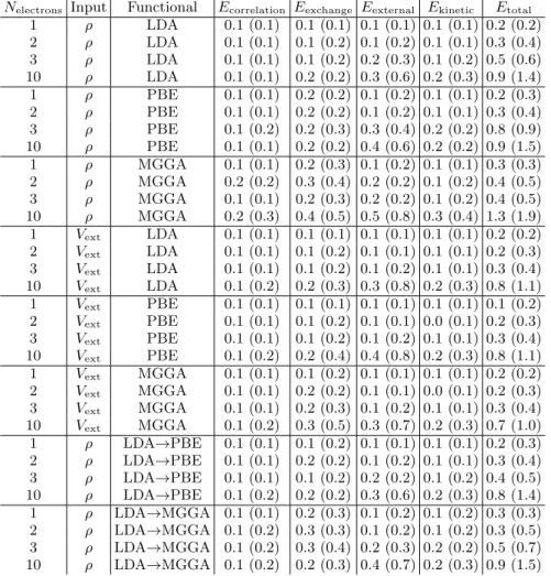
Nelectrons Input Functional Ecorrelation Eexchange Eexternal Ekinetic Etotal 1 ρ LDA 0.1 (0.1) 0.1 (0.1) 0.1 (0.1) 0.1 (0.1) 0.2 (0.2) 2 ρ LDA 0.1 (0.1) 0.1 (0.2) 0.1 (0.2) 0.1 (0.1) 0.3 (0.4) 3 ρ LDA 0.1 (0.1) 0.1 (0.2) 0.2 (0.3) 0.1 (0.2) 0.5 (0.6) 10 ρ LDA 0.1 (0.1) 0.2 (0.2) 0.3 (0.6) 0.2 (0.3) 0.9 (1.4) 1 ρ PBE 0.1 (0.1) 0.2 (0.2) 0.1 (0.2) 0.1 (0.1) 0.2 (0.3) 2 ρ PBE 0.1 (0.1) 0.2 (0.2) 0.1 (0.2) 0.1 (0.1) 0.3 (0.4) 3 ρ PBE 0.1 (0.2) 0.2 (0.3) 0.3 (0.4) 0.2 (0.2) 0.8 (0.9) 10 ρ PBE 0.1 (0.1) 0.2 (0.2) 0.4 (0.6) 0.2 (0.2) 0.9 (1.5) 1 ρ MGGA 0.1 (0.1) 0.2 (0.3) 0.1 (0.2) 0.1 (0.1) 0.3 (0.3) 2 ρ MGGA 0.2 (0.2) 0.3 (0.4) 0.2 (0.2) 0.1 (0.2) 0.4 (0.5) 3 ρ MGGA 0.1 (0.1) 0.2 (0.3) 0.2 (0.2) 0.1 (0.2) 0.4 (0.5) 10 ρ MGGA 0.2 (0.3) 0.4 (0.5) 0.5 (0.8) 0.3 (0.4) 1.3 (1.9) 1 Vext LDA 0.1 (0.1) 0.1 (0.1) 0.1 (0.1) 0.1 (0.1) 0.2 (0.2) 2 Vext LDA 0.1 (0.1) 0.1 (0.2) 0.1 (0.1) 0.1 (0.1) 0.2 (0.3) 3 Vext LDA 0.1 (0.1) 0.1 (0.2) 0.1 (0.2) 0.1 (0.1) 0.3 (0.4) 10 Vext LDA 0.1 (0.2) 0.2 (0.3) 0.3 (0.8) 0.2 (0.3) 0.8 (1.1) 1 Vext PBE 0.1 (0.1) 0.1 (0.1) 0.1 (0.1) 0.1 (0.1) 0.1 (0.2) 2 Vext PBE 0.1 (0.1) 0.1 (0.2) 0.1 (0.1) 0.0 (0.1) 0.2 (0.3) 3 Vext PBE 0.1 (0.1) 0.1 (0.2) 0.1 (0.2) 0.1 (0.1) 0.3 (0.4) 10 Vext PBE 0.1 (0.2) 0.2 (0.4) 0.4 (0.8) 0.2 (0.3) 0.8 (1.1) 1 Vext MGGA 0.1 (0.1) 0.1 (0.2) 0.1 (0.1) 0.1 (0.1) 0.2 (0.2) 2 Vext MGGA 0.1 (0.1) 0.2 (0.2) 0.1 (0.1) 0.0 (0.1) 0.2 (0.3) 3 Vext MGGA 0.1 (0.1) 0.2 (0.3) 0.1 (0.2) 0.1 (0.1) 0.3 (0.4) 10 Vext MGGA 0.1 (0.2) 0.3 (0.5) 0.3 (0.7) 0.2 (0.3) 0.7 (1.0) 1 ρ LDA→PBE 0.1 (0.1) 0.1 (0.2) 0.1 (0.1) 0.1 (0.1) 0.2 (0.3) 2 ρ LDA→PBE 0.1 (0.1) 0.2 (0.2) 0.1 (0.2) 0.1 (0.1) 0.3 (0.4) 3 ρ LDA→PBE 0.1 (0.1) 0.1 (0.2) 0.2 (0.2) 0.1 (0.2) 0.4 (0.5) 10 ρ LDA→PBE 0.1 (0.2) 0.2 (0.2) 0.3 (0.6) 0.2 (0.3) 0.8 (1.4) 1 ρ LDA→MGGA 0.1 (0.1) 0.2 (0.3) 0.1 (0.2) 0.1 (0.2) 0.3 (0.3) 2 ρ LDA→MGGA 0.1 (0.2) 0.3 (0.3) 0.1 (0.2) 0.1 (0.2) 0.3 (0.5) 3 ρ LDA→MGGA 0.1 (0.2) 0.3 (0.4) 0.2 (0.3) 0.2 (0.2) 0.5 (0.7) 10 ρ LDA→MGGA 0.1 (0.2) 0.2 (0.3) 0.4 (0.7) 0.2 (0.3) 0.9 (1.5)

TABLE II. Mean absolute errors (in mHa per electron) and root mean squared errors (in parenthesis) for models trained in this

report for the SHO potentials. The abbreviationsρ, andVext are charge density, and potential respectively. The arrows (i.e.

LDA→PBE) indicate that the charge density used as input to the DNN was calculated using the LDA exchange-correlation functional, but the labels (energies) were calculated using another exchange-correlation functional.

(13)

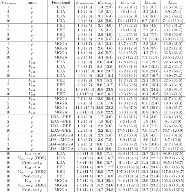
Appendix C: Mean absolute errors with the RND external potentials

(14)

Nelectrons Input Functional Ecorrelation Eexchange Eexternal Ekinetic Etotal 1 ρ LDA 0.9 (1.5) 1.4 (2.3) 14.5 (31.7) 2.5 (3.7) 14.5 (31.1) 2 ρ LDA 1.1 (2.0) 1.8 (3.1) 9.6 (19.4) 2.2 (3.4) 9.9 (25.4) 3 ρ LDA 2.0 (3.5) 3.1 (5.4) 35.1 (57.0) 5.6 (8.6) 36.1 (58.4) 10 ρ LDA 2.0 (3.8) 3.0 (5.9) 73.4 (117.1) 6.7 (10.2) 74.4 (119.4) 1 ρ PBE 1.9 (2.5) 3.1 (4.0) 15.3 (32.2) 3.8 (4.9) 15.1 (31.2) 2 ρ PBE 1.3 (2.1) 1.9 (3.1) 9.5 (19.3) 2.2 (3.1) 10.1 (21.7) 3 ρ PBE 2.0 (3.3) 2.9 (4.9) 34.4 (55.6) 5.2 (7.7) 35.6 (56.8) 10 ρ PBE 1.9 (3.6) 2.8 (5.5) 73.7 (115.0) 7.6 (11.4) 75.0 (117.1) 1 ρ MGGA 1.0 (1.7) 2.1 (3.4) 13.7 (30.7) 2.5 (3.8) 13.9 (31.0) 2 ρ MGGA 1.3 (2.2) 2.6 (4.6) 10.0 (17.8) 2.4 (3.9) 10.2 (17.8) 3 ρ MGGA 1.8 (2.8) 3.6 (5.7) 34.1 (55.7) 4.7 (7.1) 36.5 (62.2) 10 ρ MGGA 2.2 (4.1) 4.4 (8.4) 77.2 (122.1) 7.3 (11.3) 78.5 (126.1) 1 Vext LDA 5.3 (9.0) 8.6 (14.4) 17.8 (28.7) 11.5 (19.2) 22.3 (36.8) 2 Vext LDA 5.3 (8.7) 8.5 (13.6) 18.5 (31.8) 8.8 (13.5) 21.2 (33.4) 3 Vext LDA 10.6 (15.0) 16.8 (23.7) 46.2 (70.2) 15.8 (23.6) 43.2 (66.7) 10 Vext LDA 6.6 (9.9) 10.3 (15.4) 50.3 (86.1) 10.5 (16.7) 40.9 (73.2) 1 Vext PBE 6.0 (9.9) 9.3 (15.2) 17.2 (27.3) 12.1 (19.3) 22.5 (35.6) 2 Vext PBE 6.0 (9.7) 9.0 (14.7) 19.5 (32.8) 10.0 (15.4) 21.3 (34.0) 3 Vext PBE 10.9 (15.3) 16.8 (23.8) 46.1 (69.5) 16.3 (24.2) 43.6 (65.4) 10 Vext PBE 7.1 (10.6) 10.8 (16.1) 49.3 (85.4) 10.4 (16.8) 39.4 (71.5) 1 Vext MGGA 5.7 (9.8) 12.0 (20.4) 16.1 (25.3) 10.9 (17.9) 21.7 (34.8) 2 Vext MGGA 5.4 (8.6) 11.0 (17.8) 14.8 (23.2) 8.1 (12.4) 19.3 (30.0) 3 Vext MGGA 11.1 (15.5) 22.9 (32.3) 44.5 (67.9) 16.7 (25.0) 43.0 (65.7) 10 Vext MGGA 7.3 (10.8) 15.0 (22.2) 50.8 (88.0) 10.8 (16.9) 41.4 (76.0) 1 ρ LDA→PBE 1.2 (2.0) 1.7 (3.0) 14.5 (31.1) 2.4 (3.6) 14.6 (30.5) 2 ρ LDA→PBE 1.2 (4.3) 1.8 (6.4) 8.6 (19.3) 1.9 (4.6) 9.1 (23.9) 3 ρ LDA→PBE 1.9 (3.4) 2.8 (5.0) 34.8 (56.2) 5.1 (7.7) 35.6 (56.9) 10 ρ LDA→PBE 2.2 (4.0) 3.2 (6.1) 75.5 (118.4) 7.6 (11.7) 76.7 (120.9) 1 ρ LDA→MGGA 1.4 (2.8) 2.9 (5.8) 14.2 (30.9) 2.6 (4.5) 14.7 (31.6) 2 ρ LDA→MGGA 1.5 (3.7) 3.0 (7.5) 8.0 (15.2) 2.0 (4.3) 8.7 (19.6) 3 ρ LDA→MGGA 2.9 (5.4) 6.0 (11.3) 36.3 (58.2) 5.8 (10.0) 37.7 (59.8) 10 ρ LDA→MGGA 2.6 (4.9) 5.3 (9.9) 73.6 (115.6) 7.5 (11.7) 74.4 (117.4) 10 Vext→ρ LDA 6.4 (11.0) 9.9 (17.1) 93.0 (151.4) 12.7 (21.5) 98.9 (167.5)

10 Vext→ρ(DDE) LDA 6.4 (10.7) 10.0 (16.7) 99.4 (154.4) 13.4 (22.2) 108.2 (175.5)

10 Predictedρ LDA 5.8 (10.1) 9.0 (15.7) 91.4 (143.2) 11.2 (19.1) 98.5 (158.7)

10 Vext→ρ PBE 7.2 (11.7) 10.9 (17.7) 100.4 (164.8) 14.5 (24.6) 108.1 (185.8)

10 Vext→ρ(DDE) PBE 7.2 (11.5) 10.9 (17.7) 107.0 (168.1) 15.1 (24.9) 117.6 (193.7)

10 Predictedρ PBE 6.8 (11.1) 10.2 (16.8) 98.2 (151.5) 12.4 (21.4) 106.7 (170.3)

10 Vext→ρ MGGA 7.5 (12.3) 15.4 (25.1) 94.6 (161.9) 13.0 (22.8) 103.3 (180.5)

10 Vext→ρ(DDE) MGGA 7.4 (12.0) 15.2 (24.6) 101.1 (162.4) 13.7 (23.3) 111.8 (184.0)

10 Predictedρ MGGA 7.1 (12.1) 14.7 (24.8) 94.9 (150.2) 12.7 (21.5) 102.5 (167.3)

TABLE III. Mean absolute errors (in mHa per electron) and root mean squared errors (in parenthesis) for models trained in this

report for the RND potentials. The abbreviationsρ,Vext, and Predictedρare charge density, potential, and predicted charge

density respectively. The arrows (i.e. LDA→PBE) indicate that the charge density used as input to the DNN was calculated using the LDA exchange-correlation functional, but the labels (energies) were calculated using another exchange-correlation

functional. The acronym DDE stands for density driven error, as defined by Brockherde et al. [17]. The models labelled by

Vext→ρdirectly map the external potentials to charge densities. The models labelled by Predicted ρmap predicted charge