Using Visual Speech Information in Masking
Methods for Audio Speaker Separation
Faheem Khan, Ben Milner and Thomas Le Cornu
Abstract—This work examines whether visual speech infor-mation can be effective within audio masking-based speaker separation to improve the quality and intelligibility of the target speech. Two visual-only methods of generating an audio mask for speaker separation are first developed. These use a deep neural network to map visual speech features to an audio feature space from which both derived binary masks and visually-derived ratio masks are estimated, before application to the speech mixture. Secondly, an audio ratio masking method forms a baseline approach for speaker separation which is extended to exploit visual speech information to form audio-visual ratio masks. Speech quality and intelligibility tests are carried out on the visual-only, audio-only and audio-visual masking methods of speaker separation at mixing levels from -10dB to +10dB. These reveal substantial improvements in the target speech when applying the visual-only and audio-only masks, but with highest performance occurring when combining audio and visual information to create the audio-visual masks.
Index terms - speaker separation, audio-visual processing, binary masks, ratio mask
I. INTRODUCTION
This work addresses the problem of single channel audio speaker separation by investigating how visual speech information can be exploited to improve extraction of a target speaker from a mixture of speakers using masking methods. For this work, we take visual speech information to refer to information that has been extracted from a speaker’s visual speech articulators which primarily means features extracted from a video of the mouth or face. Humans are very good at extracting a target speaker from a mixture of interfering speakers. Having two ears is beneficial and to some extent this has been replicated in speaker separation systems that use multiple microphones [1]. Furthermore, humans are also able to exploit visual speech information taken from a target speaker to improve separation. However, use of this modality is much less well studied in masking methods for speaker separation and so the aim of this work is to explore how visual speech information can be exploited. In particular, visual-only methods of speaker separation are considered first before extending to combined audio-visual methods of speaker separation.
Many audio methods of speaker separation have been proposed (e.g. [2], [3], [4], [5], [6], [7], [8]), while the number of methods that utilise visual speech information is fewer (e.g. [9], [10], [11], [12], [13]). When only a single audio channel
F. Khan is with the School of Computing Sciences, University of East Anglia, UK e-mail: [email protected]
B. Milner is with the School of Computing Sciences, University of East Anglia, UK e-mail: [email protected]
T. Le Cornu is with the School of Computing Sciences, University of East Anglia, UK e-mail: [email protected]
is available the separation problem is severely underdetermined and requires constraints and assumptions to be imposed. The proposed work is based on time-frequency masking which has been effective in suppressing interfering speakers and extracting a target speaker, and was proposed originally within computational auditory scene analysis (CASA) [2], [14]. Binary masking sets mask values to 1 or 0 depending upon whether a time-frequency region is target or interference dominated, with each region of the original mixture subsequently retained or removed. Ideal binary masks (where the mask is known in advance) are highly effective in extracting a target speaker from a mixture of speakers at SNRs as low as -20dB [15]. In practice, however, the binary mask must be estimated from the input mixture. Methods to estimate masks typically first extract features from the speech mixture and then em-ploy classification methods to determine whether each time-frequency component is target or interference dominated. An early approach combined amplitude modulation spectrogram (AMS) features with two Gaussian mixture models (GMMs) to make a Bayesian classification for each time-frequency region as being target or interference dominated and achieved improvements in intelligibility [16]. Further related works continued with classification-based approaches and extracted pitch-based features and AMS features which were input into multi-layer perceptrons (MLPs), support vector machines (SVMs) and deep neural networks (DNNs) to determine each time-frequency region of the mask [17], [18]. A further study investigated 16 different acoustic features and identified a multi-resolution cochleagram feature as giving highest classification performance [19].
A shortcoming of binary masks occurs when errors lead to removal of target speech regions or retention of interference dominated regions. Several studies have shown that instead of setting each mask value to 0 or 1, better performance can be obtained using a soft, or ratio, mask. Now, each mask region takes a value in the range 0 to 1, and rather than retaining or removing a time-frequency component, a fraction is retained which is typically proportional to the local signal-to-noise ratio (SNR), and has similarity to frequency-domain Wiener filtering [1]. One approach begins by using binary masking to estimate target and interfering signals which are then used to create a ratio mask [6]. Alternatively, in [20], a recurrent neural network (RNN) is used to extract the target and interfering signals from a mixture which are then used to produce a soft time-frequency mask. In other studies the ratio mask is estimated directly from a set of features extracted from the audio mixture using DNNs [21]. Probabilistic methods of ratio masking have also been successful and model log spectral features of signals in the mixture and then make a minimum mean square error (MMSE)
estimate of the ratio mask [4], [5]. This has been compared to binary masking and shown to make more effective use of prior knowledge of speech amplitudes. In fact, in several comparative evaluations, ratio masking is shown to outperform binary masking [8], [21], [22].
A motivation of the proposed work is to examine how visual speech information can be used in mask estimation for speaker separation. This is motivated by studies that have shown correlation to exist between audio and visual speech features [23], [24], [25], [26], [27] and by advances in audio-visual speech processing [9], [10], [28], [29], [30], [31], [32], [33]. Visual speech information has taken many different forms and includes active shape model (ASM) and active appearance model (AAM) features, 2-D discrete cosine transform (DCT) features and sieve features [10], [34], [35]. These features have been used within audio speech enhancement to create visually-derived Wiener filters to improve speech quality [9], [10]. Several methods for including visual speech information into multi-channel speaker separation systems have also been developed which perform visual stream analysis that provides additional information to microphone arrays [13], [36]. For binaural audio, an audio-visual masking method has been developed that uses a power law transformation to fuse masks estimated from audio and visual streams [37]. For single-channel audio, visual speech features taken from target and interfering speakers have been used to estimate filterbank features which are subsequently combined to create a visually-derived ratio mask [11]. This audio-visual correlation has also been exploited successfully in other applications that have traditionally been based solely on audio signals. For example, robust speech recognition in noise has benefited from visual features that are insensitive to noise [28], [29]. Further applications of visual speech features include voice activity detection, voicing classification and visual-to-audio conversion where no audio is available [30], [31], [32], [38].
The aim of this work is to examine how visual speech information can be incorporated into an existing audio-based method of mask estimation to extract a target speaker from an interfering speaker. Many methods of mask estimation have been proposed (e.g. [2], [3], [4], [5], [6], [7], [8]) but few exploit information from visual speech. Of the audio-visual speaker separation and speech enhancement methods that have been proposed (e.g. [39], [40]), these typically estimate a clean audio signal, rather than a mask, from audio features taken from the mixture and from visual features extracted from the speaker. In this work, we instead use the audio estimates taken from the visual features of each speaker to create either a binary mask or ratio mask. Our previous work on visually-derived masks used GMMs to map from visual features [41]. We now improve this mapping using a deep neural network framework and present experiments and analysis to determine the effectiveness of speaker separation using just visual speech information. Furthermore, we compare our approach of mask estimation to a direct visual to mask approach that is based on methods used in several audio-only mask estimation systems [21]. We then take an effective audio-only masking method, [5], and combine this with visual masking methods to create an audio-visual mask that we show to outperform both audio and
visual only masking methods. The analysis includes speech quality and intelligibility measures and considers also the effect of gender in the mixtures and reveals the visual features to be less sensitive than audio features.
The proposed methods assume that the audio mixture from the speakers is collected from a single microphone. Visual speech features are extracted from the mouth region of each speaker in the mixture. Several example scenarios can be envisaged with such a system. A first scenario uses a single microphone and camera, possibly located together, to extract audio and video. The video captured by the camera will contain all speakers in the mixture, from which each speaker can be identified and tracked, such as in [42], [43]. Visual features for each speaker can then be extracted. A second scenario again uses a single microphone, but now uses individual cameras with each capturing video from each speaker in the mixture. These cameras could again be located centrally or positioned locally to capture video from where speakers would be located. The approach considered in this work follows the second scenario where individual cameras are used, although the techniques proposed could equally be applied to a single camera, given suitable face tracking [42], [43].
The paper is structured as follows. Section II discusses the selection of audio and visual speech features and then explains the proposed method for estimating audio features from visual speech features using a deep neural network. The two visual-only methods of speaker separation, namely binary masking and ratio masking, are described in Section III. Section IV presents the audio-visual speaker separation method which extends an audio-only ratio masking method. Experimental results and analysis are presented in Section V.
II. AUDIO FEATURE ESTIMATION
This work proposes to exploit visual speech information for mask estimation by first extracting visual features from each speaker in the mixture. Audio speech features are subsequently estimated for each speaker from the corresponding visual features and are then used within the proposed mask estimation methods. To maximise mask accuracy it is important to select a suitable visual speech feature that, when used within estimation, can yield a reliable audio speech feature.
A. Audio and visual speech features
Several studies have analysed audio and visual speech features and have shown significant correlation to exist, suffi-cient to allow audio speech features to be estimated from visual speech features [10], [23], [44]. Specifically, broad spectral envelope features such as log filterbank or mel-frequency cepstral coefficients (MFCCs) can be estimated from visual features. However, estimation of fine spectral detail, such as harmonic structure, is not possible from visual features as they lack necessary source information.
1) Audio speech features: Based on previous analysis into audio-visual correlation, mel-filterbank audio features are used in this work [10]. These are extracted from 20ms Hann windowed frames, taken at 10ms intervals, using a Fourier transform to create magnitude spectral frames,|X(t, k)|, where
300 350 400 450 −500 −450 −400 −350 −300 x y −100 0 100 −100 −50 0 50 100 xproc y proc
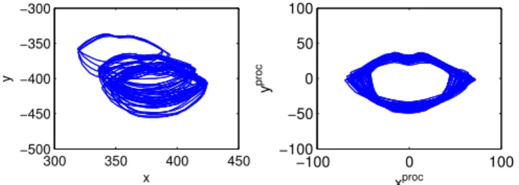
Fig. 1. Procrustes analysis for normalising lip contours to translation, scale and rotation. The left plot shows an example set of 40 outer lip contours before normalisation and the right plot shows the effect of normalisation.
k indicates the spectral bin and t is the frame index. A D-channel mel-filterbank (where D=23, from [10]) and log transform are then applied to give log filterbank vectors,
a(t) = [a(t,1), . . . , a(t, d), . . . , a(t, D)].
2) Visual speech features: Visual features are also extracted from each speaker in the mixture. Many different visual speech features have been proposed and include pixel-based and model-pixel-based approaches [45]. Considering their correlation to audio features and their widespread use in many visual speech processing applications, active appearance model (AAM) features are selected as the visual feature [34].
The AAM is trained from a set of images that have been hand-labelled with 34 2-D vertices that delineate the lip contour of the speaker. The set of vertices for each image is first normalised to create a mean lip contour using Procrustes analysis, which compensates for variations in the position of the mouth, for the size of the mouth due to varying distances of the speaker from the camera and for rotation due to the angle of the speaker’s head. This involves translating the position of each lip contour to be centred about the origin, scaling the lip contour to a mean contour size and rotating the lip contour to be orientated to a mean lip orientation [46]. The process is illustrated in Figure 1 and shows a set of outer lip contours before (left-hand side) and after normalisation (right-hand side). Following normalisation, the 34 pairs of co-ordinates are stacked to create a 68-D vector, r.
From the set of co-ordinate vectors extracted from the training images, principal components analysis (PCA) is applied which allows each co-ordinate vector to be represented as
r= ¯r+Pss (1)
where r¯ is the mean co-ordinate vector, Ps, is the set of
eigenvectors and sis a vector of coefficients that encodes the shape of the lips. To model appearance, the lip region for each training image is warped so that the points match those of the mean shape, and pixel intensities within this shape are raster scanned into vector,u. PCA is then applied which allows each pixel intensity vector to be represented as
u= ¯u+Pbb (2)
where u¯ is the mean intensity vector, Pb, is the set of
eigenvectors and bis the coefficient vector that encodes the appearance of the lips.
The shape and appearance vectors are then stacked, and a final PCA performed to decorrelate the features. The final AAM vector, o, is computed as
o=Q s b (3) where matrix Qis a PCA derived matrix that combines and compresses the shape and appearance components. For the shape and appearance vectors, the dimensionality was selected such that 98% of the total variation is captured which resulted in 30 dimensional AAM vectors.
For new images, as used in testing, a tracker automatically locates the mouth of the speaker and the AAM is fitted to this region by solving for the model parameters in (1), (2) and (3) [42], [34]. In this way, video frames are tracked and parameterised into feature vectors,o(t), that encode the visual speech at each 40ms instant, as the audio-visual database used in this work was captured at 25 video frames per second (see Section V for further details). The vectors are then upsampled to 100Hz to match the audio frame rate where each AAM vector is considered as representing the instantaneous mouth shape at 10ms intervals. First and second order derivatives, with window widths of ± 2 frames and ± 1 frame, respectively, are then augmented to produce visual vectors, v(t). These are z-score normalised to set each coefficient to have zero mean and standard deviation of one. The window widths chosen for the temporal derivatives result in information from 7 visual vectors being included, which can be considered as representing approximately 70ms of visual speech (the precise duration depends on the shutter speed used when recording the video). This was found to be a good compromise between a further small reduction in estimation error against an increase in latency.
B. Audio feature estimation from visual features
For mask estimation, the visual features from each speaker are used to estimate audio filterbank features for each speaker. Earlier work [11] used Gaussian mixture models (GMMs) for estimation but in this work it is proposed to use DNNs, given their success in a range of speech processing applications, e.g. [47], [48]. Essentially, given a visual vector, v(t), an estimate of the corresponding audio filterbank feature,aˆ(t), is made
ˆ
a(t) =f(v(t)) (4) where f is a feed-forward DNN configured for regression. The visual vector is applied to the input layer of the DNN which is passed through a number of hidden layers before the estimated filterbank vector is available on the output layer. The output from each hidden layer, and from the output layer, are a function of the output of the layer below, a set of weight connection parameters between the two layers and a bias term. A non-linearity is applied to the output of each hidden layer. This represents a fairly standard DNN implementation, as this is not the major focus of the work, but for completeness training and testing details are now given.
TABLE I
MEAN SQUARE FILTERBANK ESTIMATION ERROR USINGGMMANDDNN
METHODS FOR SPEAKERSS2, S4, S6ANDS7AND THE MEAN SQUARE OF THE REFERENCE FILTERBANKS.
S2 S4 S6 S7 Mean
GMM 1.04 1.22 1.24 1.08 1.15 DNN 0.89 0.93 0.99 0.94 0.94 Mean square 9.10 10.73 10.76 9.89 10.12
1) Training: Backpropagation of errors in conjunction with gradient descent optimisation is applied to learn a set of weight values that minimise the mean square error between the audio filterbank vector estimated from the network, aˆ(t), and the corresponding original vector,a(t). A random search over various model hyperparameters was conducted to find an optimal set [49], where the network architecture found to perform best contains four hidden layers, each with 512 units using a rectified linear unit (ReLU) activation function. The final output layer uses a linear activation function to provide the real-valued coefficient estimates. For regularisation, dropout is applied to each of the hidden layers with probability 0.5, and an l2 norm regularisation is applied with a weight of 0.001. Weights are initialised according to a uniform probability distribution in the range -0.01 to +0.01, and the learning rate is fixed at 0.0003 throughout training.
2) Accuracy of estimation: As a preliminary test, an investigation was made into filterbank estimation accuracy from visual features using the DNN, primarily to compare against the earlier method of using GMMs. Four speaker-dependent DNNs were trained, each using speech from one of four speakers in the GRID database (2 male and 2 female) with testing using a separate set of utterances from each speaker - for specific details see Section V. For each estimated filterbank vector the mean square error (MSE) was computed using the reference filterbank extracted from the clean audio and these were averaged across all frames for each speaker. To compare against our earlier work [41], the same data was used to create four 64 component speaker-dependent GMMs (which gave lowest error) and the MSE computed. Table I shows the MSE for speakers S2, S4, S6 and S7 for the DNN and GMM estimation methods. To indicate how effective filterbank estimation is relative to the reference filterbank amplitudes, the final line in Table I shows the mean square of the reference filterbank amplitudes for each speaker. For all four speakers the MSE is lower using the DNN-based system, with the average error reduced by almost 20%, which confirms the choice of using of DNNs over GMMs for estimation. Furthermore, the results also show estimation to be consistent across the four speakers.
III. VISUAL-ONLY SPEAKER SEPARATION
Two methods of visual-only mask estimation are devel-oped and explained in this section, namely visually-derived binary masks and visually-derived ratio masks. Both methods use only visual speech information to create the mask which subsequently extracts the target speaker from the mixed audio.
A. Visually-derived binary mask
Binary masking is effective at separating a target from a mixture of interfering sounds when the true, or ideal, mask is known in advance [14]. In practice, the binary mask is typically estimated from the audio mixture with many methods having been proposed [17], [18]. In this work, audio-visual correlation is exploited and a method of estimating the binary mask using visual speech information is proposed.
1) Estimation of visually-derived binary mask: A binary mask is computed from filterbank estimates of the target and interfering speakers,aˆ1 and aˆ2, obtained from corresponding visual speech features,v1andv2, extracted from each speaker in the mixture. To generate a binary mask that can be applied to the K-dimensional magnitude spectra, the D-channel log filterbank estimates are transformed to magnitude spectrum estimates,aˆ0, using an exponential operation and interpolation
ˆ
a0(t) =interp(exp(ˆa(t))) (5) Theinterpfunction uses cubic spline interpolation to convert the D-channel mel-filterbank estimate into a K-dimensional spectral estimate and takes into account the mel-spacing of the filterbank channels [50]. The magnitude spectrum binary mask,
ˆ
m(t, k), is then calculated for each time-frequency unit, as ˆ m(t, k) = 1 aˆ01(t, k) ≥λaˆ02(t, k) 0 aˆ01(t, k) <λˆa02(t, k) (6) where 1≤t≤T and 1≤k≤K, withaˆ0
1(t, k)and ˆa02(t, k) being magnitude spectrum estimates for each time-frequency unit.λallows a bias to be introduced in terms of retaining or removing time-frequency units and allows the proportion of correctly classified target-dominated regions (HITs) and false alarms (FAs) to be adjusted – see Section III-A3.
2) Extraction of target speaker: From the single channel mixed audio, 20ms Hann windowed frames are extracted at 10ms intervals and the magnitude and phase spectra computed, |Y(t, k)|and∠Y(t, k). The binary masked magnitude spectrum estimate of the target speaker,|Xb1(t, k)|, is then calculated
|X1b (t, k)|= ˆm(t, k)|Y(t, k)| 1≤t≤T, 1≤k≤K
(7) The sequence of magnitude spectral frames of the masked target speech is transformed into a continuous time-domain speech signal by combining each magnitude spectrum estimate with the phase of the original mixed speech signal, ∠Y(t, k), and applying an inverse Fourier transform. The resulting short-duration frames are then overlapped and added to create the estimate of the target speaker’s speech.
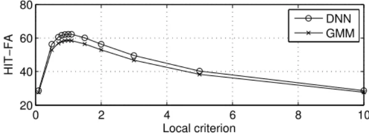
3) Analysis of mask estimation: An analysis of the visually-derived binary masking is now made and considers the effect of the threshold,λ. Performance of mask estimation is measured using the HIT-FA rate as this has been shown to be perceptually more useful than measuring classification accuracy and correlates closely with intelligibility [16], [51]. The HIT rate is the percentage of correctly classified target-dominated regions, while the FA (false alarm) rate is the percentage of wrongly classified interference-dominated regions. As the target and interfering speakers have been pre-mixed, the ideal, binary mask is known and forms the reference mask for evaluation.
As detailed in Section V, speech mixtures for evaluation are created from combinations of four speakers (two male and two female) which gives a total of 12 combinations, which are mixed at an SNR of 0dB. The HIT-FA rate is computed and then averaged across all speaker combinations and measured for λfrom 0.1 to 10 which corresponds to thresholds of -20dB to +20dB. Figure 2 shows the HIT-FA rates for each threshold and, for comparison, shows performance using filterbank features estimated using the DNN and GMM systems described in Section II-B. As a first observation, HIT-FA using the DNN is consistently higher across all values ofλcompared to the GMM, which supports the MSE analysis in Section II-B2. In terms of λ, a stable region with HIT-FA rates above 60% is achieved with0.5≤λ≤1.5with highest performance of 61% with λ= 1.0 which indicates that no bias is necessary with the 0dB SNR mixing.
Further analysis was made into mask estimation with male-male (MM), female-female (FF) and mixed-gender (MG) speech mixtures. Table II shows HIT, FA and HIT-FA rates for these combinations using DNN and GMM estimation. For all gender combinations the DNN again outperforms the GMM. Using the DNN, HIT-FA rates for all gender combinations exceed 60% with female-female slightly lower (2%) resulting from slightly higher FAs and lower HITs. This indicates that using visual speech information avoids gender biases as performance is largely consistent across all gender combinations. As a final test, we investigated an alternative approach that uses a DNN to estimate the mask directly from the visual features extracted from the two speakers (v1 and
v2). These results are shown in the final column of Table II (DNN Mask) and were obtained using the same DNN architecture described in Section II-B1 as this was found to give best performance. HIT-FA using this direct estimation is lower than when using the visual vectors to first estimate filterbanks vectors for each speaker and then create the mask. The ability of the visual features from the two speakers to create an effective audio mask relies on the DNNs being able to model the correlation between mouth shape and the audio spectral envelope. When training the DNNs no scaling was applied to the audio signals, and given that the average power of the training data for the four speakers is very similar, this effectively represents a 0dB mixing SNR case. In testing situations where the input audio power does not match that of the average power of the training data, then the log filterbank estimates can be considered as being offset by a constant term which reflects the mismatch. After transformation to the magnitude spectral domain through (5), this mismatch corresponds to a multiplicative gain term. When the audio from both speakers is scaled by the same amount (such as from a new level of amplification or by both speakers being at a new distance from the microphone) these gain terms cancel and the mask remains the same. This is a common scenario in practical situations where both speakers are likely to be close together and speaking with similar average speech powers, resulting in an SNR close to 0dB.
However, in situations where the average power of the audio from the two speakers is significantly different (such as from one speaker having a much louder voice or being closer
0 2 4 6 8 10 20 40 60 80 Local criterion HIT−FA DNN GMM
Fig. 2. Binary masking HIT-FA rates for DNN and GMM filterbank estimation for varying values ofλ.
TABLE II
HIT, FAANDHIT-FAFOR BINARY MASK ESTIMATION FROMDNNAND
GMM-BASED FILTERBANK ESTIMATES AND DIRECT ESTIMATION OF THE MASK(DNN MASK)FOR MALE-MALE(MM),FEMALE-FEMALE(FF)AND
MIXED-GENDER(MG)SPEECH MIXTURES. DNN GMM DNN Mask MM HIT 81.12 79.45 68.06 FA 18.88 20.55 14.23 HIT-FA 62.25 58.90 53.83 FF HIT 80.37 78.62 63.36 FA 19.63 21.38 13.30 HIT-FA 60.74 57.24 50.06 MG HIT 81.33 79.44 68.32 FA 18.67 20.56 14.18 HIT-FA 62.65 58.89 54.14
to the microphone), then the two gain terms will not cancel, as visual information alone cannot provide the absolute power of the audio. This corresponds to situations where the SNR takes on positive or negative values, depending on whether the target speaker has a larger or smaller average power than the interfering speaker. The impact of this can be determined from the binary masking equation (6) and the analysis made in Figure 2. These scenarios where SNRs deviate significantly from 0dB are less likely in a practical scenario, as both speakers will tend to have similar average powers, but experimental results are presented in Section V that consider both 0dB and non-0dB SNR situations.
B. Visually-derived ratio masks
Ratio masks have been proposed as a less aggressive form of binary mask that allow a fraction of the mixture to be retained in proportion to the local SNR [5], [6], [8]. The main challenge in formulating a ratio mask is knowledge of the target and interfering speakers to calculate the SNR. The implementation in this work again proposes to exploit audio-visual correlation such that audio estimates of the target and interfering speakers are obtained from the visual speech features as shown in Section II-B. Once the ratio mask has been produced a series of perceptual transforms are then considered to improve further the resulting target speech.
1) Estimation of visually-derived ratio masks: A ratio mask,RM(t, k), to extract target speech is defined as
RM(t, k) = |X1(t, k)| 2 |X1(t, k)|2+|X2(t, k)|2 = SN R(t, k) SN R(t, k) + 1 (8) where|X1(t, k)|2 and|X2(t, k)|2are the energy at time frame t and frequency bink for the target and interfering speakers
respectively and SN R(t, k) is the local SNR. Audio-visual correlation can be exploited to provide spectral envelope information from the target and interfering speakers to enable a visually-derived ratio mask to be calculated. Specifically, a spectral domain ratio mask is obtained by transforming the filterbank estimates of the target and interfering speakers, aˆ1 andaˆ2, to spectral estimates,aˆ01 andaˆ02, as shown in (5). The ratio mask to extract the target speaker is calculated as
RM(t, k) = aˆ 02 1(t, k) ˆ a02 1(t, k) + ˆa022(t, k) . (9)
2) Perceptual gain transformation: The filterbank-domain ratio mask of (9) is effective at speaker separation, but can be improved by modifying its frequency response through a perceptually-motivated transformation. Such a transformation aims to reduce distortion of the target speaker and improve suppression of the interfering speaker. This is implemented as a perceptual gain transform,Π, to give a perceptually-motivated gain,H(k), (where the time frame variable,t, has been removed for ease of notation)
H(k) = Π RM(k)
. (10)
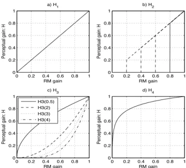
A range of perceptual gain transformations has been considered and these include piecewise and parametric functions. Four of the more effective transforms are described in (11) to (14), which defineH1 toH4, and are plotted in Figure 3.
H1(k) = RM(k) (11) H2(k) = RM(k) RM(k)> ρ 0 RM(k)≤ρ (12) H3(k) = RM(k)γ (13) H4(k) = norm log RM(k) (14)
Gain functionH1provides a baseline and is equal to the original ratio mask, RM. The second function,H2, restricts the gain so that if it falls below a threshold, ρ, then it is set to zero. This removes time-frequency regions where the SNR falls below a threshold and has similar properties to the suppression part of binary masking. Four cut-off values of ρ={0.2,0.4,0.6,0.8} are tested and give increasings levels of suppression. Gain function H3 raises the gain to the power γ which adjusts non-linearly the RM gain and is similar to the scaling method applied to the Ideal Ratio Mask (IRM) proposed in [21]. Values of γ greater than one compress the resulting gain, while γ less than one expand the gain. The fourth gain function,H4, takes the logarithm of the gain which also introduces the gain compression. The norm function is used to rescale the log gain to be in the range 0 to 1.
3) Extraction of target speaker: As described in Section III-A2, the magnitude, |Y(t, k)|, and phase,∠Y(t, k), spectra are computed from the audio mixture. The magnitude spectrum estimate of the target speaker,|X1b (t, k)|, is then calculated as
|Xb1(t, k)|=H{1,2,3,4}(t, k)|Y(t, k)| (15) 0 0.2 0.4 0.6 0.8 1 0 0.2 0.4 0.6 0.8 1 Perceptual gain: H RM gain a) H 1 0 0.2 0.4 0.6 0.8 1 0 0.2 0.4 0.6 0.8 1 Perceptual gain: H RM gain b) H 2 0 0.2 0.4 0.6 0.8 1 0 0.2 0.4 0.6 0.8 1 Perceptual gain: H RM gain c) H3 0 0.2 0.4 0.6 0.8 1 0 0.2 0.4 0.6 0.8 1 Perceptual gain: H RM gain d) H4 H3(0.5) H3(2) H3(3) H3(4)
Fig. 3. Gain mapping functions showing transformation from ratio mask,
RM, to perceptual gain functionsH1toH4, as defined in Eqs. (11) to (14).
where H{1,2,3,4}(t, k) is one of the four perceptual gain functions. As before, the magnitude spectrum estimates are combined with the phase of the mixed speech,∠Y(t, k), an inverse Fourier transform taken followed by overlapping and adding to produce the estimate of the target speech.
IV. AUDIO-VISUAL SPEAKER SEPARATION
The approach taken for audio-visual mask estimation begins by considering existing audio-only mask estimation methods in terms of their effectiveness and suitability for combination with visual speech information and included [4], [5], [21]. An initial experiment was conducted to compare a minimum mean square error (MMSE) ratio mask estimation method, based on the mixture-maximisation assumption [5], with a DNN approach that estimates a ratio mask from the input mixture [21]. The input to the MMSE method is a log spectral feature, extracted from the mixture of speakers, and the output is an estimate of the log spectral feature of the target speaker - further details are given in Section IV-A. The DNN method follows broadly the approach in [21], with some differences primarily to make a fair comparison between the two approaches. Specifically, a DNN is trained to map a stack of five input log spectral features (the same as those used in the MMSE method) to a ratio mask. The mask is then applied to the noisy mixture to estimate the target speaker spectral features, following the procedure used in (7).
The experimental set-up and evaluation metrics used to compare the two methods are the same as used for the main experiments described in Section V, with the tests conducted at an SNR of 0dB. Table III shows SDR, SIR, SAR, PESQ and STOI for the two methods and for no compensation (NC). For the majority of metrics the MMSE method outperforms the DNN approach, resulting in less distortion and interference, and slightly better speech quality. The exception is SAR, which
TABLE III
COMPARISON OFMMSE [5]ANDDNN [21]METHODS OF AUDIO-ONLY SPEAKER SEPARATION.
Method SDR SIR SAR PESQ STOI NC 0.41 0.41 279.08 1.89 0.75 MMSE 5.80 9.15 9.21 2.11 0.80 DNN 4.93 6.87 9.43 2.09 0.80
indicates that slightly more artefacts are produced by the MMSE method. Based on these results, the MMSE method was chosen to be the basis for audio-visual speaker separation. A brief description of this method is now given before consideration as to how visual information can be included.
A. Audio-only mask estimation
In the time-domain, speech from a target speaker and interfering speaker are assumed to be additive to create the time-domain mixture. From time-domain signals, short-time log spectral vectors are extracted, wherex1(k)andx2(k)represent thekth log spectral amplitudes extracted from speakers 1 and 2 respectively, andy(k)is extracted from the mixture of the two speakers. To simplify notation, we have omitted the time frame variable, t, while in practice the method is applied to each time frame. The ratio mask method makes an element-wise mixture-maximisation approximation of the log spectral vectors from the speakers in the mixture [52], as
y(k) = max x1(k), x2(k)
+e(k), 1≤k≤K (16) wheree(k)is the approximation error which can be modelled as zero mean Gaussian white noise with variance σ2
e(k).
The log spectral vectors for each speaker in the mixture are modelled using Gaussian mixture models (GMMs) which model the feature space of each speaker as a set of subsources. Specifically, it is assumed that speaker 1 is modelled using a set of I Gaussian subsources, S1 ={s1=i|i= 1,2, . . . , I} and speaker 2 is modelled as a set of J subsources, S2 =
{s2=j|j= 1,2, . . . , J}, as px1|s1(x1|s1=i) = K Y k=1 N x1(k), µi1(k), σ21i(k) (17) px2|s2(x2|s2=j) = K Y k=1 Nx2(k), µj2(k), σ22j(k) (18) where µi 1(k), µ j 2(k), σ12i(k) and σ 2j
2 (k) are the means and variances of speakers 1 and 2 for subsources i and j. Each subsource from the target speaker has prior probability, ps1(s1 = i|i = 1,2, . . . , I), and for the interfering speaker,
ps2(s2=j|j= 1,2, . . . , J). Training of the GMMs to estimate the prior probabilities, means and variances used the Linde-Buzo-Gray (LBG) algorithm for initialisation followed by expectation-maximisation (EM) which was terminated either when no change occurred or after 25 iterations [53]. Initial experiments using a validation test set found best performance with I = J = 256 subsources to model the target and interfering speakers. In practice a GMM is trained in isolation for each speaker in the mixture and we apply no normalisation to the data.
A minimum mean square error (MMSE) estimate of each element of the target speaker’s log spectral vector,xˆ1(k), can be made from the conditional expectation giveny, as
ˆ x1(k) =E(x1(k)|y) = Z x1(k) x1(k)p(x1(k)|y)dx1(k), 1≤k≤K (19) The conditional probability,p(x1(k)|y), can be written as p(x1(k)|y) =X
i,j
p(x1(k)|y, s1=i, s2=j)p(s1=i, s2=j|y) (20) which gives the estimate of x1(k)as
ˆ x1(k) = X i,j Z x1(k) x1(k)p(x1(k)|y, s1=i, s2=j)dx1(k) ×p(s1=i, s2=j|y). (21)
This comprises two factors and can be viewed as a weighted summation of the conditional estimate ofx1(k)by the posterior probability,p(s1=i, s2=j|y), of the two subsourcesi and j giveny. In practice, summing across allI×J combinations of subsources is computationally expensive and instead, as suggested in [5], the MMSE estimate is made from just the most probable pair of subsources, i∗ andj∗, that maximize the posterior probability, i.e. {i∗, j∗} = arg max
i,jp(s1 = i, s2=j|y). Following the derivation in [5], the subsources are computed as,
{i∗, j∗}= arg min i,j 1 2 X k h y(k)−max µi 1(k), µ j 2(k) 2 σ2 max(k)
+ logσ2max(k)i−logp(s1=i)−logp(s2=j). (22)
whereσ2
max(k)is the variance of the subsource (i orj) with the larger mean. This simplification can now be applied to (21), where the estimate of the target is reduced to,
ˆ x1(k) = ( Ay(k) +Bµi∗ 1(k) ifµi ∗ 1(k)≥µ j∗ 2 (k) µi1∗(k) ifµ1i∗(k)< µj2∗(k) (23) with A= σ 2i∗ 1 (k) σ2i∗ 1 (k) +σ2e(k) and B= σ 2 e(k) σ2i∗ 1 (k) +σ2e(k) . (24) where σ2i∗
1 (k) is the variance of the i∗th subsource from speaker 1 and σ2
e(k) is the variance of the approximation
error defined in (16). This shows that the estimate of the target speaker is computed in two ways depending on whether the mean component of the target speaker from thei∗th subsource, µi∗
1(k), is greater or less than the mean of the interfering speaker from thej∗th subsource,µj2∗(k). In binary masking, the estimate is set to either the mixed signal,y(k), or to zero. With this ratio mask approach, when the target speaker mean exceeds the interfering speaker mean, the estimate is now a Wiener filter-like estimate that considers both the mixed signal, y(k), and target speaker mean,µi1∗(k). Conversely, when the target speaker mean is less than the interfering speaker mean, the output is set to the target speaker mean. This is considered to be a better estimate than that in binary masking which
assumes that in this situation the target speaker is completely masked and sets the output to zero. Finally, the time-domain signal is computed by taking an inverse Fourier transform of the target spectral estimate combined with the phase of the speech mixture.
B. Audio-visual mask estimation
The audio-only ratio mask method is now extended to include visual speech information with the aim of improving the mask. Beginning with (23), visual information is included in two ways: 1) when the target mean component is less than the interfering speaker component (i.e. µi∗
1(k)< µ
j∗
2 (k)), and 2) when the target mean component is greater than the interfering speaker component (i.e. µi∗
1(k) ≥ µ
j∗
2 (k)). This leads to a modified version of (23) that incorporates visual speech information as,
ˆ x1(k) = (1−β)Ay(k) +Bµi∗ 1 (k) +βxV 1(k) ifµi ∗ 1 (k)≥µ j∗ 2 (k) (1−α)µi∗ 1 (k) +αxV1(k) ifµi ∗ 1 (k)< µ j∗ 2 (k) (25)
Considering first the situation where the target mean is less than interfering mean, i.e. the lower part of (25) where µi∗
1 (k) < µ
j∗
2 (k). The estimate, x1ˆ (k), is now refined to become a combination of the target mean, µi1∗(k), and a weighted estimate of the target speaker’s audio, xV1(k), that is derived from the corresponding visual speech feature, v1, extracted from the target speaker’s mouth. The weighting term, α, allows the contribution made by the visually-derived component, xV
1(k), in the estimation ofxˆ1(k), to be adjusted. Two methods are considered to provide the audio estimate, xV
1(k). The first method uses directly the log of the magnitude spectral estimate made from the visual feature in (4) and (5), i.e.
xV
1 = log(aˆ01). The second method uses the spectral estimate made from the visually-derived ratio mask method in (15) as the visually-derived estimate
xV1(k) =log|Xˆ1(t, k)| 1≤k≤K (26) Considering now the situation where the target mean is greater than interfering mean, i.e. the upper part of (25) where µi∗
1 (k)≥µ
j∗
2 (k). The audio-only method in (23) estimates the target,x1ˆ (k), from a Wiener-like weighting of the target mean, µi1∗(k), and the input mixture,y(k). This is also be refined to include visually-derived information, xV1(k), by introducing a second weighting term,β, to adjust the contribution made from visual information. Again, the visually-derived term,xV1(k), can be taken directly from the audio vector or from the output of the ratio mask.
V. EXPERIMENTAL RESULTS
Experiments first investigate visual-only methods of binary masking and ratio masking. Audio-visual methods are then investigated and compared against the best performing visual-only and audio-only methods. All experiments are performed using speech taken from the GRID corpus which comprises audio-visual speech recordings taken from 30 speakers, with each providing 1000 sentences [54], and sampled
at 25 video frames per second. Speech from two male speakers (S2 and S6) and two female speakers (S4 and S7) are used for the experiments. Of the 1000 utterances spoken by each speaker, 800 are used for training and the remaining 200 for testing. Speech mixtures are created using data from pairs of speakers which gives 12 different combinations of target and interfering speaker (i.e. 8 male/female combinations, 2 male/male combinations and 2 female/female combinations) which contain 2400 test utterances.
The test scenario assumes that the two speakers are talking simultaneously and located close together. Video is captured from each speaker with a separate camera. The mixed audio is created by taking speech from the target speaker and mixing it with speech from the interfering speaker that has been scaled to create the desired SNR. For each pair of speakers, utterances are mixed randomly to avoid any bias in the results. To measure the effectiveness of speaker separation in terms of quality, four measures are used, namely the source-to-distortion ratio (SDR), source-to-interference ratio (SIR), source-to-artefacts ratio (SAR) and the ITU standard objective measure of quality, namely PESQ [55], [56]. The SDR measures the amount of distortion present in the estimate of the target speech that arises from the interfering speaker, noise and artefacts introduced during separation. The SIR indicates how much of the interfering speaker remains in the target speech, while the SAR measures the level of artefacts present in the target speech. The intelligibility of the target speech is also considered and this is measured using the short-time objective intelligibility measure (STOI) which has been shown to correlate closely with subjective intelligibility measures [57].
A. Visual-only masking
The first set of experiments examines the effectiveness of the visual-only binary mask and ratio-mask/perceptual gain function methods of speaker separation. Binary masking (BM) is implemented as in (6). Ratio masks combined with perceptual gain functionsH1 toH4, as in (11) to (12), are investigated and referred to as methods RM1–RM4. For H2 andH3 the effect of ρandγ is investigated.
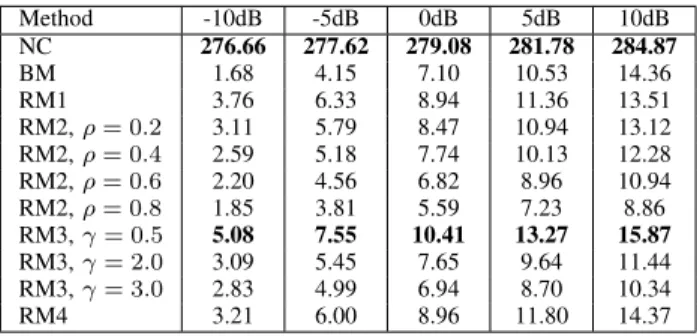
Tables IV to VIII show SDR, SIR, SAR, PESQ and STOI for the various masking methods and for no compensation (NC) at SNRs from -10dB to 10dB, with results from the 12 speaker combinations averaged to give a single score. The results show that binary masking (BM) is mainly inferior to ratio masking (RM1), a result that has also been reported in audio-only methods of masking for speaker separation [21]. Applying a perceptual gain transform (i.e. moving from RM1 to RM2, RM3, RM4) generally improves performance although this varies according to SNR and performance measure, with no single transform consistently being best. RM2, in effect, combines the ratio mask and binary mask by setting the output to zero if the gain is below the thresholdρ, with RM1 equivalent to ρ= 0. Asρis increased, more mask values are set to zero and hence more regions of the output signal are removed. This reduces the SDR, SAR, PESQ and STOI as increasing amounts of the target signal become lost. Conversely, SIR improves as ρincreases, as more time-frequency regions become removed which removes associated interferences that improves the SIR.
TABLE IV
SDRS OF VISUAL-ONLY METHODS OF SPEAKER SEPARATION. Method -10dB -5dB 0dB 5dB 10dB NC -8.41 -4.27 0.41 5.30 10.26 BM 0.21 2.63 5.31 8.38 11.81 RM1 -0.03 3.27 6.44 9.34 11.94 RM2,ρ= 0.2 0.02 3.23 6.32 9.16 11.70 RM2,ρ= 0.4 0.15 3.18 6.07 8.72 11.13 RM2,ρ= 0.6 0.38 3.09 5.63 7.97 10.12 RM2,ρ= 0.8 0.59 2.86 4.85 6.62 8.33 RM3,γ= 0.5 -1.60 2.11 5.87 9.47 12.80 RM3,γ= 2.0 0.89 3.71 6.27 8.55 10.59 RM3,γ= 3.0 1.16 3.70 5.94 7.91 9.71 RM4 -0.82 2.60 6.01 9.26 12.25 TABLE V
SIRS OF VISUAL-ONLY METHODS OF SPEAKER SEPARATION. Method -10dB -5dB 0dB 5dB 10dB NC -8.41 -4.27 0.41 5.30 10.26 BM 9.28 10.26 11.44 13.34 16.06 RM1 4.26 7.52 10.94 14.44 17.92 RM2,ρ= 0.2 5.24 8.25 11.46 14.78 18.12 RM2,ρ= 0.4 6.48 9.31 12.29 15.34 18.43 RM2,ρ= 0.6 8.09 10.62 13.34 16.07 18.78 RM2,ρ= 0.8 10.14 12.47 14.72 16.87 18.99 RM3,γ= 0.5 0.80 4.47 8.35 12.33 16.34 RM3,γ= 2.0 7.41 10.28 13.23 16.17 19.05 RM3,γ= 3.0 8.95 11.62 14.30 16.91 19.42 RM4 3.49 6.60 9.99 13.55 17.18
Considering now RM3, which raises the ratio mask gain to the power γ. RM1 is equivalent to RM3 withγ= 1, with γ= 0.5boosting gain whileγ >1suppresses gain. Examining SDRs, as SNRs increase, highest performance occurs with reducing γ, which is equivalent to reducing gain at low SNRs and increasing gain at higher SNRs. When gain is suppressed (γ >1) this reduces the contribution of the interfering speaker and so improves SIRs. Higher SAR, PESQ and STOI occur when gain is boosted (γ = 0.5) which consequently retains more of the target speaker. Interestingly, a scaling of 0.5 was also reported to give best performance when applied to an IRM proposed in [21]. RM4 also boosts gains and has a similar performance trend across performance metrics to RM3 (ρ= 0.5), although has lower overall quality and intelligibility.
These results have shown that using solely visual speech information to create masks, it is possible to improve the quality and intelligibility of the output speech over the situation with no compensation (NC). The exception is SAR, which is highest with NC as any processing introduces attributes into the signal, although of the masking methods RM3 (ρ= 0.5) gives best SAR. It may be possible to further improve performance by combining perceptual gain functions although this has not been tested formally. In terms of identifying a best performing visual masking method, highest intelligibility (STOI) and quality (as measured using PESQ) is attained consistently with RM3 (γ= 0.5). For the other measures, no single approach is best across all SNRs, although ratio masking is clearly better than binary masking.
B. Audio-visual masking
The next experiments consider audio-visual speaker separation. The first experiments examine the effect of adjusting
TABLE VI
SARS OF VISUAL-ONLY METHODS OF SPEAKER SEPARATION. Method -10dB -5dB 0dB 5dB 10dB NC 276.66 277.62 279.08 281.78 284.87 BM 1.68 4.15 7.10 10.53 14.36 RM1 3.76 6.33 8.94 11.36 13.51 RM2,ρ= 0.2 3.11 5.79 8.47 10.94 13.12 RM2,ρ= 0.4 2.59 5.18 7.74 10.13 12.28 RM2,ρ= 0.6 2.20 4.56 6.82 8.96 10.94 RM2,ρ= 0.8 1.85 3.81 5.59 7.23 8.86 RM3,γ= 0.5 5.08 7.55 10.41 13.27 15.87 RM3,γ= 2.0 3.09 5.45 7.65 9.64 11.44 RM3,γ= 3.0 2.83 4.99 6.94 8.70 10.34 RM4 3.21 6.00 8.96 11.80 14.37 TABLE VII
PESQOF VISUAL-ONLY METHODS OF SPEAKER SEPARATION. Method -10dB -5dB 0dB 5dB 10dB NC 1.20 1.52 1.89 2.18 2.54 BM 1.10 1.41 1.76 2.12 2.46 RM1 1.71 1.95 2.19 2.45 2.68 RM2,ρ= 0.2 1.47 1.72 1.98 2.24 2.49 RM2,ρ= 0.4 1.33 1.59 1.84 2.10 2.35 RM2,ρ= 0.6 1.22 1.45 1.70 1.95 2.20 RM2,ρ= 0.8 1.08 1.28 1.50 1.72 1.95 RM3,γ= 0.5 1.76 2.04 2.32 2.61 2.88 RM3,γ= 2.0 1.50 1.72 1.96 2.19 2.42 RM3,γ= 3.0 1.37 1.60 1.83 2.05 2.28 RM4 1.69 1.93 2.16 2.40 2.63
the relative contribution of the audio and visual components in deriving the ratio mask, by varyingαandβ in (25). Next, a comparison is made between audio-only, visual-only and audio-visual methods of speaker separation which considers the effect of different gender combinations in the mixture.
1) Effect ofα: The effect of changing the contribution of visual information when the target speaker mean is less than the interfering speaker mean (i.e. µi1∗(k) < µ
j∗
2 (k)) in (25) is now examined in the ratio mask by varying α. For these tests,β is set to zero so no visual information is used when the target speaker mean is greater than the interfering speaker mean (i.e.µi∗
1(k)≥µ
j∗
2 (k)). In addition, the tests also compare taking the visual estimate, xV1(k) in (25), directly from the visual vector (i.e. (5)) or from the ratio mask estimate (RM1), i.e. (26). Note, although Section V-A has shown that superior performance over the ratio mask can be achieved with a perceptual gain function for some situations (e.g. RM3, γ= 0.5), we use RM1 to make analysis more straightforward.
TABLE VIII
STOIOF VISUAL-ONLY METHODS OF SPEAKER SEPARATION. Method -10dB -5dB 0dB 5dB 10dB NC 0.56 0.65 0.75 0.83 0.89 BM 0.58 0.65 0.73 0.82 0.88 RM1 0.70 0.75 0.80 0.85 0.88 RM2,ρ= 0.2 0.67 0.73 0.78 0.83 0.87 RM2,ρ= 0.4 0.64 0.70 0.76 0.81 0.85 RM2,ρ= 0.6 0.61 0.66 0.72 0.77 0.82 RM2,ρ= 0.8 0.58 0.62 0.67 0.71 0.76 RM3,γ= 0.5 0.72 0.78 0.83 0.88 0.92 RM3,γ= 2.0 0.65 0.70 0.75 0.80 0.84 RM3,γ= 3.0 0.62 0.67 0.72 0.77 0.81 RM4 0.68 0.74 0.80 0.85 0.89
0 0.1 0.2 0.3 0.4 0.5 0.6 0.7 0.8 0.9 1 5 6 7 8 9 10 α SDR, SIR, SAR 0 0.1 0.2 0.3 0.4 0.5 0.6 0.7 0.8 0.9 11.5 1.7 1.9 2.1 2.3 2.5 PESQ SDR−DV SDR−RM SIR−DV SIR−RM SAR−DV SAR−RM PESQ−DV PESQ−RM (a) 0 0.2 0.4 0.6 0.8 1 0.75 0.8 0.85 α STOI STOI−DV STOI−RM (b)
Fig. 4. Effect ofαfor direct visual (DV) and ratio mask (RM) estimates, for a) SDR, SIR, SAR (left axis) and PESQ (right axis), and b) STOI.
That said, in further analysis in Section V-B3, we compare RM1 with RM3. Figure 4a shows SDR, SIR, SAR and PESQ scores and Figure 4b shows STOI scores, both computed for 0 ≤ α ≤ 1 with xV
1(k) estimated directly from the visual vector (DV) and from the ratio mask (RM) at an SNR of 0dB.
Setting α = 0 is equivalent to the audio-only ratio mask method in (23). Increasing α beyond zero increases the contribution of the visual information up to α= 1where the contribution is solely from the visual estimate. As a first observation, using the ratio mask (RM) estimate in (25) gives higher performance than the direct visual (DV) estimate due to it providing a better estimate of the audio feature. Secondly, as the contribution made by the visual component increases, performance improves although when weighting too much towards visual the performance reduces as the information in the visual features is not sufficient to maintain performance. The proportion,α, of visual information for peak performance varies across the different measures and is in the range0.4≤α≤0.9. For further tests a value of α= 0.5 is used together with the ratio mask for providing xV
1(k)in (25).
2) Effect of β: The effect of varying the contribution of visual information is now examined when the target speaker mean is greater than the interfering speaker mean (i.e.µi∗
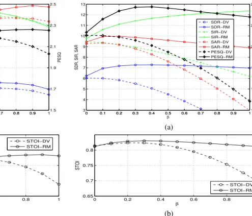
1(k)≥ µj2∗(k)) where increasingβ in (25) increases the proportion of visual information. The tests again compare the the effect of estimatingxV1 from either the direct visual estimate or the ratio mask estimate. Figure 5a shows SDR, SIR, SAR and PESQ scores and Figure 5b shows STOI scores, both computed for 0≤β≤1, withα= 0.5. 0 0.1 0.2 0.3 0.4 0.5 0.6 0.7 0.8 0.9 1 3 4 5 6 7 8 9 10 11 12 13 β SDR, SIR, SAR 0 0.1 0.2 0.3 0.4 0.5 0.6 0.7 0.8 0.9 11.5 1.7 1.9 2.1 2.3 2.5 PESQ SDR−DV SDR−RM SIR−DV SIR−RM SAR−DV SAR−RM PESQ−DV PESQ−RM (a) 0 0.2 0.4 0.6 0.8 1 0.65 0.7 0.75 0.8 β STOI STOI−DV STOI−RM (b)
Fig. 5. Effect ofβfor direct visual (DV) and ratio mask (RM) estimates, for a) SDR, SIR, SAR (left axis) and PESQ (right axis), and b) STOI.
The results show that using the ratio mask to provide xV1 is again better than estimation directly from the visual vector and secondly that best performance occurs when using a smaller proportion of visual information than when the target speaker mean is less than the interfering speaker mean (Figure 4). When the target mean is greater than the interfering mean it is likely that the audio component in the mixture is closer to the target speech than when the target mean is less than the interfering mean. Therefore, adjusting this potentially more accurate audio component by the less accurate DV-based visual estimate tends to degrade the resulting estimate in comparison to using the more accurate estimate from the ratio mask. In the situation where the target mean is less than the interfering mean (Figure 4), the audio component in the mixture is likely to be a poorer estimate of the target speech, so adjusting this by the less accurate DV-based visual estimate has a smaller impact. Highest SDR, SAR, PESQ and STOI scores occur with 0.3≤β ≤0.5 which is a lower range of values than found when optimising forα. This equates to using less contribution from the visual information whenµi∗
1 (k)≥µ j∗ 2 (k)and more contribution when µi∗ 1(k)< µ j∗
2 (k). This is again attributed to the audio component in the mixture being closer to the target speaker when the target speaker mean is greater than the interfering speaker mean, and hence less contribution is required from the visual information. Conversely, when the target speaker mean is less than the interfering speaker mean, the visual information is more useful, hence the observation ofα > β for best performance. We also performed a similar analysis using RM3 (γ= 0.5). This showed a similar trend in performance with again the observation ofα > β and values
TABLE IX
SDRS OF AUDIO AND VISUAL METHODS OF SPEAKER SEPARATION. Method -10dB -5dB 0dB 5dB 10dB NC -8.41 -4.27 0.41 5.30 10.26 AUDIO 0.94 3.42 5.80 8.68 11.78 RM1 -0.03 3.27 6.44 9.34 11.94 RM3 -1.60 2.11 5.87 9.47 12.80 AVα RM1 1.29 3.94 6.24 9.28 12.74 AVα RM3 0.85 3.60 6.14 8.87 11.94 AVβ RM1 2.71 4.88 7.27 10.14 13.44 AVβ RM3 1.85 4.37 7.01 9.75 12.50 TABLE X
SIRS OF AUDIO AND VISUAL METHODS OF SPEAKER SEPARATION. Method -10dB -5dB 0dB 5dB 10dB NC -8.41 -4.27 0.41 5.30 10.26 AUDIO 5.41 7.33 9.15 11.60 14.57 RM1 4.26 7.52 10.94 14.44 17.92 RM3 0.80 4.47 8.35 12.33 16.34 AVα RM1 6.00 8.12 9.76 11.65 14.52 AVα RM3 4.47 6.93 9.12 11.52 14.52 AVβ RM1 7.74 9.76 11.71 14.76 17.92 AVβ RM3 5.38 7.82 10.47 13.39 16.71
of α= 0.5 andβ= 0.4giving best performance.
3) Comparison of methods: A comparison of the audio-only, visual-only and audio-visual mask estimation methods is now made across a range of SNRs from -10dB to 10dB. As a baseline the original audio-only ratio masking method (AUDIO) is used, as was overviewed in Section IV-A. For visual-only methods the ratio mask methods of RM1 and RM3 (γ= 0.5) are used. Two audio-visual methods are considered. Method AVα is based on (25) and uses visual information only when the target speaker mean is less than the interfering speaker mean. Method AVβ extends AVα and uses visual information when the target speaker mean is also greater than the interfering speaker mean. The two audio-visual methods are combined with RM1 and RM3 to give four systems, AVα RM1, AVα RM3, AVβ RM1 and AVβ RM3.
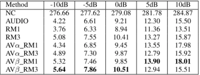
Tables IX to XIII show SDR, SIR, SAR, PESQ and STOI scores for the seven systems and for no compensation (NC). Comparing audio-only and visual-only methods (RM1 and RM3) shows the best performing method to vary with SNR and metric. Audio-only mask estimation gives higher SDR at low SNRs but is outperformed by visual-only masks at higher SNRs. Visual-only mask estimation using RM1 outperforms RM3 at all SNRs for SIRs but the converse is true for SAR, PESQ and STOI. For these measures RM3 generally outperforms only mask estimation. Comparing visual masks to the audio-visual masks reveals AVαto give higher scores across almost all combinations of SNR and performance measures as a result of combining audio and visual information for mask estimation when the target mean is less than the interfering mean. By utilising visual information in all mask estimates, AVβ further improves performance and attains highest performance at all SNRs and for all five performance measures, with specific performance dependent on whether the RM1 or RM3 is used. As a further test, the effect of the gender of the two speakers in the mixture is examined for the audio-only, visual-only (RM1) and audio-visual (AVβ RM1) methods. Using the
TABLE XI
SARS OF AUDIO AND VISUAL METHODS OF SPEAKER SEPARATION. Method -10dB -5dB 0dB 5dB 10dB NC 276.66 277.62 279.08 281.78 284.87 AUDIO 4.22 6.61 9.21 12.30 15.50 RM1 3.76 6.33 8.94 11.36 13.51 RM3 5.08 7.55 10.41 13.27 15.87 AVα RM1 4.34 6.85 9.45 13.55 17.98 AVα RM3 4.89 7.30 9.87 12.79 15.92 AVβ RM1 5.32 7.46 9.85 13.90 18.01 AVβ RM3 5.64 7.86 10.51 12.94 15.51 TABLE XII
PESQOF AUDIO AND VISUAL METHODS OF SPEAKER SEPARATION. Method -10dB -5dB 0dB 5dB 10dB NC 1.20 1.52 1.89 2.18 2.54 AUDIO 1.80 1.98 2.11 2.37 2.59 RM1 1.71 1.95 2.19 2.45 2.68 RM3 1.76 2.04 2.32 2.61 2.88 AVα RM1 1.82 2.04 2.26 2.45 2.70 AVα RM3 1.88 2.07 2.30 2.44 2.65 AVβ RM1 2.06 2.26 2.45 2.69 2.91 AVβ RM3 2.07 2.25 2.45 2.67 2.89
two male and two female speakers, separate SDR, SIR, SAR, PESQ and STOI scores are measured for male-male (MM), female-female (FF) and mixed gender (MG) combinations at an SNR of 0dB with results and error bars shown in Figure 6. In terms of SDR, a large difference is observed between male-male mixtures compared to female-female and mixed gender mixtures when using audio-only masking. For visual-only masking, male-male separation is much improved, and performance across all three gender combinations is much closer which suggests visual masking is less sensitive to gender than audio masking. With audio-visual separation, the improvement of male-male separation with visual-only masking is maintained while female-female and mixed gender separation improve further. SIR and SAR measurements show similar trends to that for SDR, although differences between gender combinations are less. Considering PESQ and STOI, with audio-only separation lower performance is observed for same gender combinations than for mixed gender. With visual-only separation, STOI and PESQ scores are improved across same gender mixtures, and for audio-visual separation the highest performance for all gender combinations is attained.
VI. CONCLUSION
The aim of this work has been to investigate whether visual speech information can be used to aid mask estimation
TABLE XIII
STOIOF AUDIO AND VISUAL METHODS OF SPEAKER SEPARATION. Method -10dB -5dB 0dB 5dB 10dB NC 0.56 0.65 0.75 0.83 0.89 AUDIO 0.74 0.78 0.80 0.86 0.90 RM1 0.70 0.75 0.80 0.85 0.88 RM3 0.72 0.78 0.83 0.88 0.92 AVα RM1 0.75 0.78 0.81 0.87 0.91 AVα RM3 0.76 0.79 0.83 0.87 0.90 AVβ RM1 0.78 0.80 0.83 0.88 0.92 AVβ RM3 0.78 0.81 0.85 0.88 0.92
Audio Visual AV 3 4 5 6 7 8 a) SDR Audio Visual AV 4 6 8 10 12 14 b) SIR Audio Visual AV 6 7 8 9 10 11 c) SAR Audio Visual AV 1.5 2 2.5 d) PESQ Audio Visual AV 0.75 0.8 0.85 e) STOI MM FF MG
Fig. 6. Male-male (MM), female-female (FF) and mixed-gender (MG) speaker separation using audio-only, visual-only and audio-visual methods showing a) SDR, b) SIR, c) SAR, d) PESQ and e) STOI, with standard error bars shown.
for audio speaker separation. Estimation of audio features from visual features, that will subsequently be used within mask estimation, was found to be more accurate when moving from GMMs to DNNs. It may be that more sophisticated neural network architectures will achieve more accurate audio features, and subsequently better masks, but this is beyond the scope of this paper. The subsequent binary masks and ratio masks, computed solely from visual features, were found to be able to extract target speech from a mixture of speakers. The models used to map from visual to audio features were trained with speech data that had similar average powers which results in masks that can be considered as assuming a mixture SNR of 0dB. This works well for situations where the two speakers are equidistant from the microphone and have similar loudnesses. However, when the audio power from the two speaker differs, the absolute powers, which the visual features are unable to represent, reduces the accuracy of the mask. In such circumstances, supplementary information regarding the SNR could be used to scale the audio amplitudes estimated from the visual features, and could employ methods such as an audio-visual voice activity detector to estimate the SNR [31]. Compared to audio-only ratio masks, the resulting target speech from visually-derived masks was found to be of generally slightly lower quality and intelligibility. Audio-visual masking was then proposed to combine the audio and visual masks into an audio-visual mask. Evaluation found this to give highest performance across all methods tested and across all SNRs.
REFERENCES
[1] B. Widrow and S. Stearns,Adaptive signal processing. Prentice-Hall, 1985.
[2] D. Wang and G. J. Brown,Computational Auditory Scene Analysis: Principles, Algorithms, and Applications. Wiley-IEEE Press, 2006. [3] S. Roweis, “Factorial models and refiltering for speech separation and
denoising,” inEurospeech, 2003, pp. 1009–1012.
[4] A. Reddy and B. Raj, “Soft mask methods for single-channel speaker separation,”IEEE Trans. Audio, Speech and Language Processing, vol. 15, no. 6, pp. 1766–1776, Aug. 2007.
[5] M. Radfar and R. Dansereau, “Single-channel speech separation using soft mask filtering,”IEEE Trans. Audio, Speech and Language Processing, vol. 15, no. 8, pp. 2299–2310, Nov. 2007.
[6] D. Williamson, Y. Wang, and D. Wang, “Reconstruction techniques for improving the perceptual quality of binary masked speech,”Journal of the Acoustical Society of America, vol. 136, no. 2, pp. 892–902, Aug. 2014.
[7] X.-L. Zhang and D. Wang, “A deep ensemble learning method for monaural speech separation,”IEEE Trans. Audio, Speech and Language Processing, vol. 24, no. 5, pp. 967–977, May 2016.
[8] D. Wang and J. Chen, “Supervised speech separation based on deep learning: An overview,” CoRR, vol. abs/1708.07524, 2017. [Online]. Available: http://arxiv.org/abs/1708.07524
[9] L. Girin, J.-L. Schwartz, and G. Fang, “Audio-visual enhancement of speech in noise,”Journal of the Acoustical Society of America, vol. 109, no. 6, pp. 3007–3020, Jun. 2001.
[10] I. Almajai and B. Milner, “Visually derived Wiener filters for speech enhancement,”IEEE Trans. Audio, Speech and Language Processing, vol. 19, no. 6, pp. 1642–1651, Aug. 2011.
[11] F. Khan and B. Milner, “Speaker separation using visual speech features and single-channel audio,” inInterspeech, 2013.
[12] J. Hershey and M. Casey, “Audio-visual sound separation via hidden Markov models,” inProc. Neural Information Processing Systems, 2001. [13] B. Rivet, W. Wang, S. Naqvi, and J. Chambers, “Audiovisual speech source separation: An overview of key methodologies,”IEEE Signal Processing Magazine, vol. 31, no. 3, pp. 125–134, May 2014. [14] G. Hu and D. Wang, “Monaural speech segregation based on pitch
tracking and amplitude modulation,” IEEE Trans. Neural Networks, vol. 15, no. 5, pp. 1135–1150, Sep. 2004.
[15] N. Li and P. Loizou, “Factors influencing intelligibility of ideal binary-masked speech: Implications for noise reduction,” Journal of the Acoustical Society of America, vol. 123, no. 3, pp. 1673–1682, Mar. 2008.
[16] G. Kim, Y. Lu, Y. Hu, and P. Loizou, “An algorithm that improves speech intelligibility in noise for normal-hearing listeners,”Journal of the Acoustical Society of America, vol. 126, no. 3, pp. 1486–1494, Sep. 2009.
[17] Z. Jin and D. Wang, “A supervised learning approach to monaural segregation of reverberant speech,” IEEE Trans. Audio, Speech and Language Processing, vol. 17, no. 4, pp. 625–638, May 2009. [18] K. Han and D. Wang, “A classification based approach to speech
segregation,” Journal of the Acoustical Society of America, vol. 132, no. 5, pp. 3475–3483, Nov. 2012.
[19] J. Chen, Y. Wang, and D. Wang, “A feature study for classification-based speech separation at low signal-to-noise ratios,” IEEE Trans. Audio, Speech and Language Processing, vol. 22, no. 12, pp. 1993–2002, Dec. 2014.
[20] P.-S. Huang, M. Kim, M. Hasegawa-Johnson, and P. Smaragdis, “Joint optimization of masks and deep recurrent neural networks for monaural source separation,”IEEE Trans. Audio, Speech and Language Processing, vol. 23, no. 12, pp. 2136–2147, Dec. 2015.
[21] Y. Wang, A. Narayanan, and D. Wang, “On training targets for supervised speech separation,”IEEE Trans. Audio, Speech and Language Processing, vol. 22, no. 12, pp. 1849–1958, Dec. 2014.
[22] A. Morris, J. Barker, and H. Bourlard, “From missing data to maybe useful data: soft data modelling for robust ASR,” inProc. Workshop Upon Innovation in Speech Processing, Stratford-upon-Avon, Apr. 2001. [23] H. Yehia, P. Rubin, and E. Vatikiotis-Bateson, “Quantitative association of vocal tract and facial behavior,”Speech Communication, vol. 26, no. 1, pp. 23–43, Oct. 1998.
[24] J. Barker and F. Berthommier, “Evidence of correlation between acoustic and visual features of speech,” inICPhS, 1999, pp. 199–202. [25] I. Almajai, B. Milner, and J. Darch, “Analysis of correlation between
audio and visual speech features for clean audio feature prediction in noise,” inInterspeech, 2006, pp. 2470–2473.
[26] C. Chandrasekaran, A. Trubanova, S. Stillittano, A. Caplier, and A. Ghazanfar, “The natural statistics of audiovisual speech,” PLoS Computational Biology, vol. 5, no. 7, pp. 1–17, 2009.
[27] J. Peelle and M. Sommers, “Prediction and constraint in audiovisual speech perception,”Cortex, vol. 68, pp. 169–181, 2015.
[28] G. Potamianos, C. Neti, J. Luettin, and I. Matthews, “Audio-visual automatic speech recognition: An overview,” Issues in Audio-Visual Speech Processing, MIT Press, 2004.
[29] V. Estellers, M. Gurban, and J.-P. Thiran, “On dynamic stream weighting for audio-visual speech recognition,”IEEE Trans. Audio, Speech and Language Processing, vol. 20, no. 4, pp. 1145–1157, May 2012.
[30] P. Liu and Z. Wang, “Voice activity detection using visual information,”
Proc. ICASSP, pp. 609–612, 2004.
[31] I. Almajai and B. Milner, “Using audio and visual features for robust voice activity detection in clean and noisy speech,” inEUSIPCO, 2008. [32] T. le Cornu and B. Milner, “Generating intelligible audio speech from visual speech,”IEEE Trans. Audio, Speech and Language Processing, vol. 25, no. 9, pp. 1751–1761, Sep. 2017.
[33] ——, “Reconstructing intelligible audio speech from visual speech features,” inInterspeech, Sep. 2015.
[34] T. F. Cootes, G. J. Edwards, and C. J. Taylor, “Active appearance models,”
IEEE Trans. on Pattern Analysis and Machine Intelligence, vol. 23, no. 6, pp. 681–685, June 2001.
[35] Y. Lan, R. Harvey, B. Theobald, E.-J. Ong, and R. Bowden, “Comparing visual features for lipreading,” inAVSP, 2009, pp. 102–106.
[36] S. Shivappa, B. Rao, and M. Trivedi, “Audio-visual fusion and tracking with multilevel iterative decoding: Framework and experimental eval-uation,”IEEE Journal of Selected Topics in Signal Processing, vol. 4, no. 5, pp. 882–894, Oct. 2010.
[37] Q. Liu, W. Wang, P. Jackson, M. Barnard, J. Kittler, and J. Chambers, “Source separation of convolutive and noisy mixtures using audio-visual dictionary learning and probabilistic time-frequency masking,”IEEE Trans. Signal Processing, vol. 61, no. 22, pp. 5520–5535, Nov. 2013. [38] T. le Cornu and B. Milner, “Voicing classification of visual speech using
convolutional neural networks,”Proc. FAAVSP, 2015.
[39] Z. Wu, S. Sivadas, Y. K. Tan, M. Bin, and R. S. M. Goh, “Multi-modal hybrid deep neural network for speech enhancement,”CoRR, vol. abs/1606.04750, 2016.
[40] J.-C. Hou, S.-S. Wang, Y.-H. Lai, J.-C. Lin, Y. Tsao, H.-W. Chang, and H.-M. Wang, “Audio-visual speech enhancement using deep neural networks,” inAPSIPA, 2016.
[41] F. Khan and B. Milner, “Using audio and visual information for single channel speaker separation,” inInterspeech, 2015.
[42] E. Ong, Y. Lan, B. Theobald, R. Harvey, and R. Bowden, “Robust facial feature tracking using selected multi-resolution linear predictors,” inIn Proc. Int. Conference Computer Vision ICCV09, 2009, pp. 1483–1490. [43] F. Huang and T. Chen, “Tracking of multiple faces for human-computer interfaces and virtual environments,” inInternational Conference on Multimedia and Expo, vol. 3, 2000, pp. 1563–1566.
[44] J. Jiang, A. Alwan, P. Keating, E. Auer, and L. Bernstein, “On the relationship between face movements, tongue movements and speech acoustics,”Journal on Applied Sig. Proc., vol. 11, pp. 1174–1188, 2002. [45] Y. Lan, R. Harvey, B. Theobald, E.-J. Ong, and R. Bowden, “Comparing
visual features for lipreading,” inProc. AVSP, 2009.
[46] J. Gower, “Generalized procrustes analysis,”Psychometrika, vol. 40, pp. 33–51, 1975.
[47] T. N. Sainath, A. Mohamed, B. Kingsbury, and B. Ramabhadran, “Deep convolutional neural networks for LVCSR,” inICASSP, 2013, pp. 8614– 8618.
[48] Y. Xu, J. Du, L.-R. Dai, and C.-H. Lee, “An experimental study on speech enhancement based on deep neural networks,”IEEE Signal Processing Letters, vol. 21, no. 1, pp. 65–68, 2014.
[49] J. Bergstra and Y. Bengio, “Random search for hyper-parameter opti-mization,”The Journal of Machine Learning Research, vol. 13, no. 1, pp. 281–305, 2012.
[50] B. Milner and X. Shao, “Prediction of fundamental frequency and voicing from mel-frequency cepstral coefficients for unconstrained speech reconstruction,”IEEE Trans. Audio, Speech and Language Processing, vol. 15, no. 1, pp. 24–33, Jan. 2007.
[51] Y. Wang and D. Wang, “Towards scaling up classification-based speech separation,”IEEE Trans. Audio, Speech and Language Processing, vol. 21, no. 7, pp. 1381–1390, Jul. 2013.
[52] D. Burshtein and S. Gannot, “Speech enhancement using a mixture-maximum model,”IEEE Trans. Speech Audio Process., vol. 10, no. 6, pp. 341–351, Sep. 2002.
[53] Y. Linde, A. Buzo, and R. Gray, “An algorithm for vector quantisation design,”IEEE Trans. Commun., vol. 28, no. 1, pp. 94–95, Jan. 1980. [54] M. Cooke, J. Barker, S. Cunningham, and X. Shao, “An audio-visual
corpus for speech perception and automatic speech recognition,”Journal of the Acoustical Society of America, vol. 150, no. 5, pp. 2421–2424, Nov. 2006.
[55] E. Vincent, R. Gribonval, and C. Fevotte, “Performance measurement in blind audio source separation,”IEEE Trans. Audio, Speech and Language Processing, vol. 14, no. 4, pp. 1462–1469, July 2006.
[56] ITU-T,Perceptual evaluation of speech quality (PESQ): An objective method for end-to-end speech quality assessment of narrowband tele-phone networks and speech codecs. ITU-T recommendation P.862, 2000.
[57] C. Taal, R. Hendriks, R. Heusdens, and J. Jensen, “A short-time objective intelligibility measure for time-frequency weighted noisy speech,” in