Detecting behavioral variations in system resources of large data centers
Sara Casolari, Michele Colajanni, Stefania Tosi
University of Modena and Reggio Emilia{sara.casolari, michele.colajanni, stefania.tosi}@unimore.it Abstract—The identification of significant changes in system
resource behaviors is mandatory for an efficient management of data centers. As the dimension of modern data centers increases, the evaluation of state change detections through traditional algorithms becomes computationally intractable. We propose a novel approach that characterizes the statistical properties of the resource measures coming from system monitors, classifies them, and signals a change only when there is modification of the resource classification. This method diminishes the computational complexity and reaches the same detection accuracy of traditional approaches as demonstrated by several results obtained in real enterprise data centers.
Keywords-change detection; resource behavior; private clouds
I. INTRODUCTION
Most management systems related to enterprise data cen-ters and private cloud architectures are activated after a notification that a behavioral change has occurred in some server resource(s). Efficient management requires suitable algorithms able to take decisions on the basis of actual and past behavior of the server resources. For this reason, the most important resources are continuously monitored and data are passed to some statistical methods that decide whether to signal the occurrence of a change.
Existing models and frameworks that signal relevant changes in server operations by working on the entire data sets of monitored resources [1], [2] are inadequate to support system management decisions. We should consider that, even in a medium size infrastructure, huge amounts of data streams referring to different system resources may reach a change detector that should analyze, model and treat them at different temporal scales (from days to weeks) and should support prompt reconfigurations motivated by changes in system and workloads [3]. On the other side, solutions that avoid the analysis of all monitored measures by working on aggregated visions of subsets of heterogeneous servers [3] prevent both reliable change detections and the identification of servers that experienced that changes. Therefore, two main problems limit the applicability of present approaches for change detection and motivate this paper: dimensionality and heterogeneity of the data set.
This paper proposes a novel approach to address issues related to the identification of relevant behavioral changes in enterprise data centers that must be found on the basis of several and heterogeneous data streams. The first goal
is to consider just the most important data streams, where the importance is measured in relation to their impact on the overall system behavior. After having obtained the most rele-vant data, we classify them by distinguishing under-loaded, deterministic or random behaviors so that we characterize servers on the basis of their main behavioral nature. We take advantage of the previous characterization as a basis for evaluating the dynamic evolution at the level of servers; this periodic evaluation allows us to signal in a simple and accurate way the most significant behavioral changes.
The proposed approach has three main advantages: it does not require to model and analyze all resource measures of each server; it makes no a-priori assumptions about the statistical characteristics of data; it is flexible enough to detect behavioral changes at different time scales. These features guarantee that our method is appropriate for behav-ioral change detection in large enterprise data centers where continuous changes and high dimensionality of data are the norm.
The remainder of this paper is structured as follows. Section II presents the behavioral change problem definition and provides the necessary foundations of the proposed methodology. This is presented in Section III, where we give a detailed description of the proposed approach, by presenting the steps taken to identify relevant changes in server behavior. Section IV applies the solution to a specific case study, by characterizing the server behavior and detect-ing behavioral changes on a typical enterprise data center. Concluding remarks are presented in Section V.
II. PROBLEM DEFINITION AND FUNDAMENTAL CHOICES
Most management systems referring to enterprise data centers and private cloud architectures require algorithms that are able to decide whether a relevant change has occurred in the profile of some monitored system resources. In this context, change detection should reduce the operator involvement in favor of model-driven decision systems. Existing models and frameworks are inadequate to support management decisions that have to gather, filter and analyze huge amounts of heterogeneous and variable data streams, because they work on the entire data set of measures coming from server monitors.
The goal of the methodology of interest for this paper is to detect behavioral changes in server resource measures, in terms of a collection of related data instances that behaves
anomalously with respect to a behavior observed so far on the data stream [4]. The detection of behavioral changes requires the identification of a set of behavioral attributes and to find whether and when these attributes change. We identify the behavioral attributes in the statistical properties of monitored measures (e.g., correlation, standard deviation, mean value), that represent the type of relationship between data instances. When the observed statistical properties of a data stream significantly differ from the expected be-havior, a change is declared. Let us evidence an example of behavioral change in Figure 1. We consider the CPU utilization measures of a server hosting five virtual machines. The data show a periodic behavior during the first 1000 samples and then suddenly change to a stable behavior. This is a typical example of behavioral change that, for an efficient management of the enterprise data center, the detection algorithm should promptly signal.
0 20 40 60 80 100 0 200 400 600 800 1000 1200 Sample Values Samples
Figure 1. Example of a behavioral change.
This paper provides a methodology for detecting behav-ioral changes in large data centers and private cloud architec-tures. These systems are characterized by a high number of heterogeneous hardware and software components (proces-sors, memories, storage elements, applications) that operate at different time scales (spanning from days to entire weeks), and can be subject to prompt reconfigurations due to changes in system, security and business policies. In these conditions, our methodology addresses the challenge of detecting behav-ioral changes in suitable subsets of servers, interacting and competing for the same components at spatial, functional or application level. Our proposal works on performance measures sampled at suitable temporal intervals, ranging from seconds to few minutes in relation to the different time scales of interest. It is mandatory to remark that the proposed change detector is oriented to enterprise data centers, to the so called private cloud-based infrastructures, and to any context where the system manager has full control on the resources assigned to different services. On the other hand, in the present version, the proposed approach cannot be applied to cloud data centers where the cloud provider can
assign and move virtual machines from one host/cluster to another one without informing the cloud consumer. Our methodology signals changes when the behavior of a server departs from normality, by using two types of supports for facing the dimensionality and heterogeneity problems: the analysis of a small set of all and only informative data; the classification of streams among negligible, deterministic and random streams so to evidence their statistical behavior.
The first stage is to evaluate the impact of each data stream on the system activity, so to distinguish important and not-relevant sources of information. Eliminating the less important data streams diminishes the system management complexity. Since the resource measures in a data center may be highly variable and this characteristics influences the change detection, we consider variability as the main statistical property to discriminate between relevant and not-relevant information. The variability is typically expressed in terms of process variance or in terms of coefficient of varia-tion, and it quantifies the degree of activity of a process even as a measure of the system health. Indeed, the variability of processes is used to characterize the system behavior [5] in many different natural and non-natural processes, such as the flow of water through a river basin, the traffic of highway systems, or the Internet traffic. In [6], the process variance is used to classify heterogeneous nodes for revealing the impact of external requests on the system. In this paper, we define energy the index of variation of the monitored processes, and we use this energy information in order to characterize the statistical nature of server behaviors. We reduce the dimensionality of the data set by evaluating its variability and by applying the Principal Component
Analysis (PCA) [7] that allows us to remove low energy
information and to consider just relevant data.
As a second stage, we characterize the resource behavior emerging from the monitored data in three main categories:
• deterministic behavior, whose behavioral attributes are
systematic trends and periodic patterns that are pre-dictable and possible to model;
• random behavior, presenting isolated and occasional
bursts and dips, spikes and noises;
• negligible behavior, that gives a little contribution to
the overall system behavior.
Figures 2(a), (b) and (c) report an example of the three men-tioned statistical behaviors in the CPU utilization sampled from a Web server, an application server and a database server of the data center, respectively.
This classification is quite important because it allows us to identify the actual behavior of a server and to assign it to one of the three categories. The change in time in the characterization of a server is symptomatic of a significant behavioral change in its functioning. The identification of this type of changes is obtained through our methodology without the need of analyzing all numerous
0 10 20 30 40 50 60 70 80
Mon Tue Wed Thu Fri Sat Sun
CPU Utilization (a) Negligible 0 10 20 30 40 50 60
Mon Tue Wed Thu Fri Sat Sun
CPU Utilization (b) Random 0 10 20 30 40 50 60 70 80
Mon Tue Wed Thu Fri Sat Sun
CPU Utilization
(c) Deterministic
Figure 2. Examples of server behaviors.
and heterogeneous data streams and without the loss of relevant information.
III. METHODOLOGY
The proposed detection method employs statistical anal-yses of data developed at consecutive intervals of time in order to signal a change in the behavior of some servers. At time intervalt, the set of collected sampled measures origi-nates a matrixXtthat forms a high dimensional multivariate
structure. It is an×pmatrix, wherenis the number of sam-ples collected among two consecutive intervals (for example,
n= 2016if we consider the five minutes samples enclosed in an one-week interval), andpis the number of considered system resource measures. To each resource matrix Xt
we associate a vector Bt = [bt,1, . . . , bt,p] containing, the
characterization of each resource measure at time intervalt, that is, bt,k ∈ {Deterministic, Random, N egligible} for
1 ≤ k ≤ p. At the next time interval t+ 1, we collect the new set of observations Xt+1 and check whether the
Bt+1 vector characterizes the server behaviors as at timet.
When a relevant change affects some servers, their statistical characterization changes and Bt 6= Bt+1. This deviation
is symptomatic of a relevant change that we are able to capture simply by looking at the differences in the elements of two vectors. It is important to remark that the proposed approach shows only major changes through the analysis of a small set of data. However, a lack of change in the statistical characterization does not mean that a server did not experience any change. We now detail how to build the Bt vectors. At each time interval t, our methodology
implements two steps on collected data: dimensionality
reduction and heterogeneity inspection.
The first step is required since the data sets collected from the server log files of modern enterprise data centers form a multivariate structure characterized by thousands of dimensions and more. In these structures and associated coordinated spaces, any reliable decision requires a pre-liminary identification of the most relevant information for management purposes. A common approach is to find a new coordinate space consisting of a lower dimension that is representative of the original space [8]. When a structure can
be approximated through a smaller number of dimensions in a way that minimizes the error and the loss of information, we can refer to the smaller number of dimensions as the
structure intrinsic dimensionality. In literature [9] several
models exist. In our implementation, we choose the PCA [7] since we are mainly interested to measure the system energy in term of variance, and the PCA is the best model to reveal the intrinsic structure of data set on the basis of its variance. As data sets of resource measures are statistically hetero-geneous, before applying PCA to the collectedXtmatrix it
is important to normalize them to time series characterized by zero mean and unit variance, as suggested in [10]. PCA maps Xt on a new set of axes [8] called components.
Calculating the components is equivalent to solving the symmetric eigenvalue problem for the matrixΨt=XtTXt,
that is a measure of the covariance of the time series deriving from sampled measures. In practice, at sample i
each component vi is the i-th eigenvector computed from
the spectral decomposition of Ψt [10]:
Ψtvi = λivi i= 1, . . . , p (1)
where λi is the eigenvalue corresponding to the eigenvector vi and represents the magnitude of the variation along each
component vi. We quantify the energy, σi, associated to
the component vi as the percentage of variation related
to its eigenvalue λi, that is, σi = Pλip∗100
j=1λj. As Ψt is
symmetric positive definite, its eigenvectors are orthogonal and the corresponding eigenvalues are non-negative real numbers. By convention, the eigenvectors are unit norm and the eigenvalues are arranged from large to small, so that
λ1≥λ2≥. . .≥λp.
Once mapped the data set into their component space, we have to compute the transformed data considering one component at a time. In this new dimensional space, a
dimension ui (i= 1, . . . , p) is defined as a vector of sizep
obtained by the contribution of the data set matrixXt and
of the component vi. As suggested in [10], this vector is
each principal component vi we have: ui = Xtvi √ λi i= 1, . . . , p (2)
The above equation shows that all server behaviors, when weighted by vi, produce one dimension of the transformed
data. Thus the vector ui captures the temporal variation
common to all server measures along the component vi.
Since the components are ordered with respect to their contribution to the overall energy,u1captures the strongest
temporal trend common to all server measures,u2 captures
the next strongest, and so on.
The energy characterizing each component can be used to reduce the data dimensionality by ignoring the less variable components of the structure. In order to choose how many component it is useful to retain, we pursue the criterion of the percentage of variability expressed by the principal components [11]. We determine in advance the amount of residual variability that we want tolerate and then exclude the residual components. Finding that only a small set ofr
dimensions are relevant implies thatXtcan be mapped on a r-dimensional subspace ofRpand thatr≪pis the intrinsic dimension ofXt. At every time intervalt, this result allows
the method to distinguish between the relevant dimensions
Ut = {u1, . . . , ur} that are contributions shared by all
re-source measures on therprincipal components, and the
not-relevant dimensionsUt={ur+1, . . . , up} corresponding to
the less important components in terms of system energy. The second step investigates data heterogeneity with the goal of characterizing server behaviors at time interval t
and register in the Bt vector their deterministic, random
or negligible nature. After the classification in relevant Ut
and not-relevantUt dimensions, we distinguish the relevant
dimensions between correlated UC
t and low-correlated UtL
by evaluating the autocorrelation function (ACF) of each relevant dimension Ut as in [12] and many other
con-texts [13], [14]. Figure III(a) reports an example of dimen-sion exhibiting correlated periodicity and seasonal fluctua-tions because of diurnal activity, as well as the difference between weekday and weekend activity. The high values of the autocorrelation function of Figure III(b) confirm that the dimension is correlated. Figure III(a) reports an example of a dimension that is classified as low-correlated, since it presents the quick decay of the ACF values shown in Figure III(b). This dimension is characterized by random perturbations and/or spikes varying in time and intensity. We use the classification of the relevant dimensions between correlated and low-correlated to evaluate three behavioral values for each data stream referring to one server resource. At every time interval t and for every server resource measure k (1 ≤ k ≤ p), the idea is to add all the contributions for each of the three types of dimensions and then to evaluate the maximum.
-5 0 5 10 15 20
Mon Tue Wed Thu Fri Sat Sun
Dimension 1 (a) Dimension -0.8 -0.6 -0.4 -0.2 0 0.2 0.4 0.6 0.8 1 50 100 150 200 250 ACF ACF (b) ACF
Figure 3. Example of correlated dimension.
-40 -30 -20 -10 0 10 20 30 40 50
Mon Tue Wed Thu Fri Sat Sun
Dimension 4 (a) Dimension -0.8 -0.6 -0.4 -0.2 0 0.2 0.4 0.6 0.8 1 50 100 150 200 250 ACF ACF (b) ACF
Figure 4. Example of low-correlated dimension.
• Dt,k = Pjvj, ∀j | uj ∈ UtC denotes the contributions
provided by the relevant correlated dimensions;
• Rt,k = Pjvj, ∀j | uj ∈ UtL denotes the contributions
provided by the relevant low- correlated dimensions;
• Nt,k=Pjvj, ∀j|uj ∈Ut, accumulates the contributions
of the not-relevant dimensions.
Now, it is possible to compute the highest value among the three that is,Mt,k =max{Dt,k, Rt,k, Nt,k}, and to estimate
the characterization,bt,k, of thek-th server resource measure
on the basis of its main behavioral value: bt,k= 8 < : Deterministic ifMt,k=Dt,k Random ifMt,k=Rt,k Negligible ifMt,k=Nt,k (3)
The characterization of each server is recorded in the
Bt vector and represents the term of comparison for the
detection of a behavioral change in the characterization at two consecutive time intervals. When bt,k 6= bt+1,k, a
behavioral change affecting the k-th monitored server is detected.
IV. RESULTS
In this section, we present the experimental results of the proposed approach on data traces collected from an enterprise data center consisting of 514 servers and sup-porting different types of applications, including Web sites, databases, access controls, CMS, mail server, management software. In this testbed, system monitors collect resource measures every minute referring to CPU utilization, primary and secondary memory-related metrics, network activities. Our system is organized hierarchically, as suggested in [15], with subsystems of almost half a hundred servers in order to support an efficient orchestration of real-time management mechanisms. For the sake of presentation, we consider two
data sets,XtandXt+1, referring to the CPU utilization of a
subsystem of 50 servers hosting e-Commerce websites with dynamic and interactive content over two consecutive days, November 8 and 9, 2010, respectively. Xt and Xt+1 are
matrices with n = 1440 rows and p = 50 columns. Sec-tion IV-A presents the results of the server characterizaSec-tion and of the behavioral change detection. In Section IV-B, we analyze the computational complexity of the methodology by considering several sizes of the data set.
A. Server characterization and behavioral changes
We initially consider the matrix Xt and evaluate the
energy σi carried on by each dimension ui in order to
identify how many dimensions actually bring information to this data set. Considering the 90-percentile of the energy of the overall system, we estimate that it is captured just by the first nine dimensions as shown in Table I. These dimensions contribute to most of server variability. Our approach evaluates the first 9 dimensions as relevant, while the other 41 dimensions are marked as not-relevant from the point of view of the energy. This is an important result of the proposed methodology applied to a real data center because it confirms that, in terms of energy, the resource measures all together form a structure with an intrinsic dimensionality ofr= 9that is much lower than the original number (50) of the considered set of time series. The application of the ACF to ther= 9relevant dimensions gives that 5 dimensions are
correlated and 4 are low-correlated (Table I).
Order Behavioral class Energy
1 Correlated 51.03% 2 Correlated 11.99% 3 Correlated 8.64% 4 Low-correlated 4.8% 5 Low-correlated 3.27% 6 Correlated 3.14% 7 Correlated 3% 8 Low-correlated 2.87% 9 Low-correlated 2.42% Table I
CLASSIFICATION OF RELEVANT DIMENSIONS.
The goal is now to determine which dimensions actually bring information to which CPU traces of the data set. In the left half of Table II, we report the results of the server characterization on the data set Xt. The columns Dt, Rt
and Nt denote the three categories of our methodology at
time intervalt. Since it is important to validate the proposed approach, we compare its results against those obtained by applying to each data stream the traditional mechanisms (that we name Baseline characterization) requiring
sta-tistical methods for the analysis of server behavior, in-cluding the correlation among values [12] and probability distributions [16], and mean load analysis [17]. Due to the high variability of system resource measures, all these analyses must provide a pre-filtering step to remove noise
from data [18]. The classification results achieved by the Baseline characterization are reported in the second column. In the same table, we report the results obtained through the proposed approach in the three Methodology columns. These columns highlight in bold text theMtvalue for each
server. This value denotes the behavioral characterization that is assigned by the proposed methodology. For example, baseline analyses at time interval t of server 3 compute a mean load utilization of 6.39% that sets it as a negligible server. Our methodology reaches the same characterization through the computation of only three behavioral values: a predominantNt,3value of 0.1866 characterizes the server as
under-loaded, avoiding the analysis of the entire data stream. If we compare the classes with bold indexes to the server characterization arising from the Baseline characterization reported in the second column, we see a perfect correspon-dence of results. Indeed, our methodology is able to identify the main statistical behavior of 50 servers through a classi-fication and a statistical analysis of only the most relevant 9 dimensions of the data set. By working on dimensions that capture the common patterns of data variation and isolate random perturbations, our methodology avoids to apply any filtering techniques on the small set of dimensions.
We apply the proposed methodology on the second data setXt+1 in order to obtain the system view of the next day.
During the night, a new business application connected to a database was installed and caused a relevant change in server activities. The results are shown in the right half of Table II. By comparing the characterization results ofXt andXt+1,
we are able to evidence the behavioral changes of servers. In particular, the new application modifies the activity of servers 11, 15 and 17 from deterministic to random, as denoted by their prevailing Dt and Rt+1 values. In such
a way, we are able to evaluate the behavioral implications of the new application in the activity of servers due to the effect of non-determinism incurred by the new requests. A more detailed analysis is reported in Figure 5. Figure 5(a) shows the CPU utilization trace of the server 11 before the introduction of the new application. An evident deterministic behavior follows the diurnal activity of users. With the insertion of the new application, server 11 changes its behavior showing random dips and bursts of CPU utilization as in Figure 5(b). 0 20 40 60 80 100 Mon CPU Utilization
(a) Time intervalt
0 20 40 60 80 100 Tue CPU Utilization (b) Time intervalt+ 1 Figure 5. Behavioral change of server 11.
X
tX
t+1Baseline Methodology Baseline Methodology
characterization characterization
CPU Behavior Dt Rt Nt Behavior Dt+1 Rt+1 Nt+1
1 Random 0.2211 0.2379 0.0181 Random 0.1155 0.2592 0.0481 2 Negligible 0.0006 0.0009 0.1297 Negligible 0.0008 0.0012 0.1373 3 Negligible 0.0443 0.0334 0.1866 Negligible 0.0537 0.0454 0.1936 4 Random 0.0391 0.3012 0.1185 Random 0.0409 0.3120 0.1115 5 Negligible 0.0186 0.0116 0.1955 Negligible 0.0190 0.0163 0.2051 6 Negligible 0.0162 0.0128 0.1938 Negligible 0.0183 0.0141 0.2182 7 Random 0.0615 0.2379 0.0181 Random 0.0753 0.2622 0.0201 8 Negligible 0.0492 0.0370 0.2030 Negligible 0.0505 0.0401 0.2112 9 Random 0.1160 0.2206 0.1236 Random 0.1724 0.2310 0.1311 10 Negligible 0.0005 0.0005 0.1309 Negligible 0.0008 0.0018 0.1413 11 Deterministic 0.3539 0.1612 0.0540 Random 0.2073 0.2648 0.0208 12 Negligible 0.0099 0.0049 0.1960 Negligible 0.0133 0.0054 0.2006 13 Negligible 0.0139 0.0122 0.2052 Negligible 0.0105 0.0166 0.2922 14 Deterministic 0.3158 0.2091 0.0150 Deterministic 0.3801 0.1696 0.0117 15 Deterministic 0.2302 0.0792 0.0860 Random 0.0434 0.2309 0.0345 16 Deterministic 0.3057 0.2396 0.0176 Deterministic 0.3113 0.2601 0.0158 17 Deterministic 0.3368 0.1016 0.0402 Random 0.1556 0.2635 0.0198 18 Random 0.0357 0.3350 0.0712 Random 0.0370 0.3048 0.0525 19 Random 0.0685 0.2085 0.0071 Random 0.0484 0.2391 0.0111 20 Deterministic 0.2755 0.1612 0.0251 Deterministic 0.2444 0.1220 0.0288 21 Random 0.1170 0.2858 0.0239 Random 0.1333 0.2510 0.0244 22 Random 0.0837 0.3412 0.0213 Random 0.0745 0.3287 0.0255 23 Deterministic 0.3955 0.0846 0.0927 Deterministic 0.3446 0.0821 0.1018 24 Deterministic 0.3163 0.3154 0.0374 Deterministic 0.3131 0.3987 0.0345 25 Negligible 0.0002 0.0006 0.1037 Negligible 0.0012 0.0005 0.1198 26 Negligible 0.0569 0.0402 0.1912 Negligible 0.0722 0.0550 0.1624 27 Negligible 0.0071 0.0186 0.2028 Negligible 0.0113 0.0225 0.2888 28 Negligible 0.0220 0.0268 0.2112 Negligible 0.0245 0.0211 0.2009 29 Random 0.0432 0.1261 0.1127 Random 0.0669 0.1174 0.0990 30 Random 0.0207 0.2498 0.0137 Random 0.0193 0.2330 0.0115 31 Deterministic 0.3955 0.0846 0.0927 Deterministic 0.3566 0.0866 0.1217 32 Deterministic 0.4183 0.2324 0.0277 Deterministic 0.4033 0.2431 0.0071 33 Deterministic 0.3037 0.2695 0.0293 Deterministic 0.3169 0.2244 0.0331 34 Random 0.2114 0.2388 0.0166 Random 0.2070 0.2388 0.0166 35 Negligible 0.0478 0.0410 0.1858 Negligible 0.0552 0.0670 0.2004 36 Negligible 0.0387 0.0353 0.2114 Negligible 0.0307 0.0564 0.2145 37 Random 0.0275 0.3535 0.0616 Random 0.0222 0.3114 0.0601 38 Negligible 0.0236 0.0842 0.1214 Negligible 0.0215 0.0667 0.1552 39 Random 0.0611 0.2059 0.0287 Random 0.0021 0.2003 0.0224 40 Deterministic 0.3810 0.2160 0.0421 Deterministic 0.3911 0.2022 0.0126 41 Deterministic 0.2462 0.0784 0.0815 Deterministic 0.2132 0.0663 0.0115 42 Deterministic 0.3902 0.0892 0.0960 Deterministic 0.3888 0.0531 0.0770 43 Negligible 0.0003 0.0008 0.1094 Negligible 0.0005 0.0011 0.1677 44 Negligible 0.0039 0.0100 0.1755 Negligible 0.0023 0.0332 0.1810 45 Deterministic 0.3879 0.1695 0.0458 Deterministic 0.3552 0.1565 0.0221 46 Deterministic 0.3002 0.0716 0.0866 Deterministic 0.3441 0.0651 0.0733 47 Negligible 0.0090 0.0198 0.1659 Negligible 0.0110 0.0153 0.1977 48 Negligible 0.0221 0.0237 0.2081 Negligible 0.0319 0.0451 0.2231 49 Negligible 0.0006 0.0003 0.1388 Negligible 0.0007 0.0004 0.1874 50 Deterministic 0.2032 0.0898 0.0844 Deterministic 0.2243 0.0711 0.0491 Table II
SERVER CHARACTERIZATION AND BEHAVIORAL CHANGES.
Changes in server behaviors guide system operators to adapt the system to changing environments. Besides that, the identification of changes in the behavior of some servers does not imply a change in overall system functioning: the transition of a handful of servers from the deterministic to
the random class does not mean a necessary change in the overall system operations.
B. Computational complexity of the methodology
In this section, we evaluate the computational complexity of the proposed methodology in order to assess its feasibility
Methodology Baseline characterization
Major processing steps Computational Major processing steps Computational
involved complexity involved complexity
PCA analysis of a nxp matrix O(p3
+n∗p2) Filtering of p streams of length n O(p∗nlog(n))
Behavioral analysis of r streams O(r∗n2) Behavioral analysis of p streams O(p∗n2)
Total O(p3
+n∗p2 +r∗n2) Total O(p∗n2)
Table III
COMPUTATIONAL COMPLEXITY OF THE APPROACHES.
to data center dimensionality. We compare the number of computations required by our proposal for characterizing server behavior to that needed by traditional approaches working on the all set of monitored data. The two computa-tional complexities are reported in Table III (we remindnas the number of samples,pthe number of considered resource measures and rthe number of relevant dimensions.)
The PCA requires aroundO(p3+n
∗p2)computations [19]
for the eigenvalue decomposition of a covariance matrix, while the analysis of the statistical attributes of a stream may provide a number of operations spanning from logarithmic to exponential in the number of samples. In this evaluation, we consider the application of behavioral analyses having at most a quadratic computational cost. Hence, the total computational complexity of the proposed methodology is O(p3 + n
∗p2 + r
∗n2). On the other side, the baseline
characterization needs a pre-filtering step on all monitored data before applying behavioral analyses. Also for filtering techniques, there are a lot of models with different properties and complexities. In order to provide reliable characteriza-tions, we decide to apply Fast Fourier Transform [18] for filtering data by makingO(p∗nlog(n))computations. Then, quadratic (or less) behavioral analyses are applied to all filtered data. Hence, the total computational complexity of the baseline approach isO(p∗nlog(n)+p∗n2)
≈ O(p∗n2).
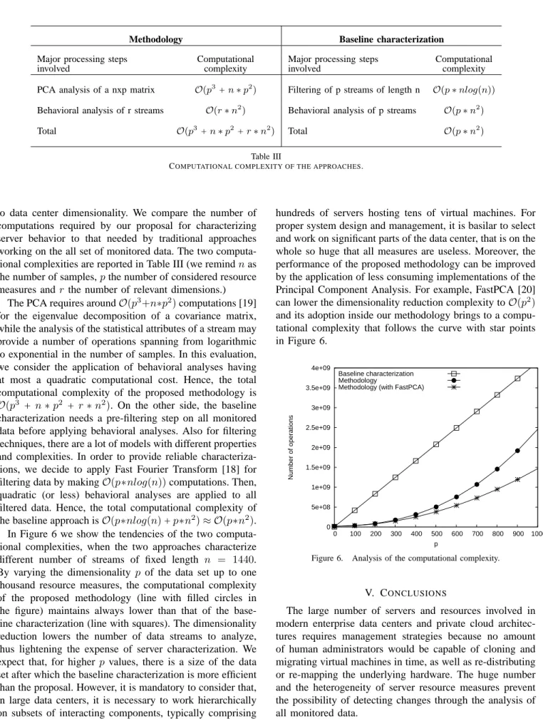
In Figure 6 we show the tendencies of the two computa-tional complexities, when the two approaches characterize different number of streams of fixed length n = 1440. By varying the dimensionality p of the data set up to one thousand resource measures, the computational complexity of the proposed methodology (line with filled circles in the figure) maintains always lower than that of the base-line characterization (base-line with squares). The dimensionality reduction lowers the number of data streams to analyze, thus lightening the expense of server characterization. We expect that, for higher pvalues, there is a size of the data set after which the baseline characterization is more efficient than the proposal. However, it is mandatory to consider that, in large data centers, it is necessary to work hierarchically on subsets of interacting components, typically comprising
hundreds of servers hosting tens of virtual machines. For proper system design and management, it is basilar to select and work on significant parts of the data center, that is on the whole so huge that all measures are useless. Moreover, the performance of the proposed methodology can be improved by the application of less consuming implementations of the Principal Component Analysis. For example, FastPCA [20] can lower the dimensionality reduction complexity toO(p2)
and its adoption inside our methodology brings to a compu-tational complexity that follows the curve with star points in Figure 6. 0 5e+08 1e+09 1.5e+09 2e+09 2.5e+09 3e+09 3.5e+09 4e+09 0 100 200 300 400 500 600 700 800 900 1000 Number of operations p Baseline characterization Methodology
Methodology (with FastPCA)
Figure 6. Analysis of the computational complexity.
V. CONCLUSIONS
The large number of servers and resources involved in modern enterprise data centers and private cloud architec-tures requires management strategies because no amount of human administrators would be capable of cloning and migrating virtual machines in time, as well as re-distributing or re-mapping the underlying hardware. The huge number and the heterogeneity of server resource measures prevent the possibility of detecting changes through the analysis of all monitored data.
In this paper, we propose a methodology for the detection of behavioral changes in modern enterprise data centers, where monitored data streams refer to heterogeneous and variable system resource measures. By providing a data dimensionality reduction and a characterization of server statistical heterogeneity, we are able to detect changes in server operations without the need of statistically analyzing the entire set of resource measures. The results achieved by applying the methodology to a real context validate our proposal and open interesting perspectives on novel decision support systems and resource management models.
REFERENCES
[1] S. Casolari, M. Colajanni, F. Lo Presti, and S. Tosi, “Real-time models supporting management decisions in highly variable systems,” in Proc. of the 29th IEEE Int. Performance,
Computing and Communications Conf., New Mexico, NM,
USA, 2010.
[2] E. Hartikainen and S. Ekelin, “Enhanced network-state esti-mation using change detection,” in Proc. of the 31st IEEE
Conf. on Local Computer Networks, Nov. 2006.
[3] X. e. a. Zhu, “1000 islands: an integrated approach to resource management for virtualized data centers,” Cluster Computing, vol. Vol. 12, no. 1, 2008.
[4] V. Chandola, A. Banerjee, and V. Kumar, “Anomaly detection: A survey,” ACM Comput. Surv., vol. 41, no. 3, pp. 1–58, 2009. [5] M. Argollo de Menezes and A. Barabasi, “Separating internal and external dynamics of complex systems,” Physical review
letters, vol. 93, no. 6, 2004.
[6] S. Casolari, M. Villani, M. Colajanni, and R. Serra, “Sep-arating internal and external fluctuation in distributed web-based services,” in Proc. of European Conference on Complex
Systems, Warwick, UK, 2009.
[7] H. Abdi and L. Williams, “Principal component analysis,”
Computational Statistics, 2010, in press.
[8] H. Hotelling, “Analysis of a complex of statistica variables into principal components,” J. Educ. Psy., pp. 417–441, 1933. [9] K. Mardia, J. Kent, and J. Bibby, Multivariate Analysis, ser. Probability and Mathematical Statistics. Academic Press, 1995.
[10] L. Anukool, K. Papagiannaki, M. Crovella, C. Diot, E. D. Kolaczyk, and N. Taft, “Structural analysis of network traffic flows,” Joint International Conference on Measurement and
Modeling of Computer Systems, pp. 61–72, 2004.
[11] J. Jackson, A user’s guide to principal components, ser. Wiley series in probability and mathematical statistics: Applied probability and statistics. Wiley, 1991.
[12] C. Chatfield, The Analysis of Time Series: An Introduction. Chapman and Hall, 1989.
[13] M. Andreolini, S. Casolari, and M. Colajanni, “Models and framework for supporting run-time decisions in web-based systems,” ACM Tran. on the Web, vol. 2, no. 3, 2008.
[14] Y. Baryshnikov, E. Coffman, G. Pierre, D. Rubenstein, M. Squillante, and T. Yimwadsana, “Predictability of Web server traffic congestion,” in Proc. of the 10th
Interna-tional Workshop on Web Content Caching and Distribution (WCW2005), Sophia Antipolis, FR, Sep. 2005.
[15] M. Andreolini, S. Casolari, and S. Tosi, “A hierarchical ar-chitecture for on-line control of private cloud based systems,” 2010.
[16] R. Gnanadesikan and M. B. Wilk, “Probability plotting meth-ods for the analysis of data,” Biometrika, vol. 55, pp. 1–17, 1968.
[17] D. Gmach, J. Rolia, L. Cherkasova, G. Belrose, T. Turicchi, and A. Kemper, “An integrated approach to resource pool management: Policies, efficiency and quality metrics,” in
Proc. of the IEEE Int. Conf. on Dependable Systems and Networks, 2008.
[18] A. V. Oppenheim, R. W. Schafer, and J. R. Buck,
Discrete-time signal processing. Prentice Hall, 1999.
[19] G. H. Golub and C. F. Van Loan, Matrix Computations (Johns
Hopkins Studies in Mathematical Sciences). The Johns Hopkins University Press, Oct. 1996.
[20] A. Sharma and K. K. Paliwal, “Fast principal component analysis using fixed-point algorithm,” Pattern Recognition