Deep Convolutional Neural Network for Inverse Problems in Imaging

(1)

Deep Convolutional Neural Network for

Inverse Problems in Imaging

Kyong Hwan Jin, Michael T. McCann, Member, IEEE, Emmanuel Froustey, and Michael Unser, Fellow, IEEE

Abstract— In this paper, we propose a novel deep convolutional neural network (CNN)-based algorithm for solving ill-posed inverse problems. Regularized iterative algorithms have emerged as the standard approach to ill-posed inverse problems in the past few decades. These methods produce excellent results, but can be challenging to deploy in practice due to factors including the high computational cost of the forward and adjoint operators and the difficulty of hyperparameter selection. The starting point of this paper is the observation that unrolled iterative methods have the form of a CNN (filtering followed by pointwise non-linearity) when the normal operator ( H∗H , where H∗ is the adjoint of the forward imaging operator, H ) of the forward model is a convolution. Based on this observation, we propose using direct inversion followed by a CNN to solve normal-convolutional inverse problems. The direct inversion encapsulates the physical model of the system, but leads to artifacts when the problem is ill posed; the CNN combines multiresolution decomposition and residual learning in order to learn to remove these artifacts while preserving image structure. We demonstrate the performance of the proposed network in sparse-view reconstruction (down to 50 views) on parallel beam X-ray computed tomography in synthetic phantoms as well as in real experimental sinograms. The proposed network outperforms total variation-regularized iterative reconstruction for the more realistic phantoms and requires less than a second to reconstruct a 512×512 image on the GPU.

Index Terms— Image restoration, image reconstruction, tomog-raphy, computed tomogtomog-raphy, magnetic resonance imaging, bio-medical signal processing, biobio-medical imaging, reconstruction algorithms.

I. INTRODUCTION

O

VER the past decades, iterative reconstruction methods have become the dominant approach to solving inverse

Manuscript received November 4, 2016; revised April 10, 2017 and May 24, 2017; accepted May 24, 2017. Date of publication June 15, 2017; date of current version July 11, 2017. This work was supported in part by the European Union’s Horizon 2020 Framework Programme for Research and Innovation under Grant 665667 (call 2015), in part by the Center for Biomedical Imaging of the Geneva-Lausanne Universities and EPFL, in part by the European Research Council under Grant 692726 (H2020-ERC Project GlobalBioIm), and in part by the National Institute of Biomedical Imaging and Bioengineering under Grant EB017095 and under Grant EB017185. The associate editor coordinating the review of this manuscript and approving it for publication was Prof. Jan Sijbers. (Corresponding author: Michael Unser.) K. H. Jin and M. Unser is with the Biomedical Imaging Group, École Poly-technique Fédérale de Lausanne, CH-1015 Lausanne, Switzerland (e-mail: [email protected]; [email protected]).

M. T. McCann is with the Center for Biomedical Imaging, Signal Processing Core and the Biomedical Imaging Group, École Polytech-nique Fédérale de Lausanne, CH-1015 Lausanne, Switzerland (e-mail: [email protected]).

E. Froustey was with the Biomedical Imaging Group, École Polytechnique Fédérale de Lausanne, CH-1015 Lausanne, Switzerland. He is now with Dassault Aviation, 92210 Saint-Cloud, France.

Color versions of one or more of the figures in this paper are available online at http://ieeexplore.ieee.org.

Digital Object Identifier 10.1109/TIP.2017.2713099

problems in imaging including denoising [1]–[3], deconvolu-tion [4], [5], and interpoladeconvolu-tion [6]. With the appearance of compressed sensing [7] and the related regularizers such as total variation [1], [2], [4], [8], robust and practical algorithms have appeared with excellent image quality and reasonable computational complexity. These advances have been partic-ularly influential in the field of biomedical imaging, e.g., in magnetic resonance imaging (MRI) [9]–[11] and X-ray computed tomography (CT) [12]–[14]. These devices face an unfavorable trade-off between noise and acquisition time. Short acquisitions lead to severe degradations of image quality, while long acquisitions may cause motion artifacts, patient discomfort, or even patient harm in the case of radiation-based modalities. Iterative reconstruction with regularization provides a way to mitigate these problems in software, i.e. without developing new scanners.

A more recent trend is deep learning [15], which has arisen as a promising framework providing state-of-the-art performance for image classification [16], [17] and segmen-tation [18]–[20]. Moreover, regression-type neural networks have demonstrated impressive results on inverse problems with exact models such as signal denoising [21], [22], deconvolu-tion [23], artifact reducdeconvolu-tion [24], [25], signal recovery (model-based restoration) [26], [27], and interpolation [28]–[30]. Central to this resurgence of neural networks has been the convolutional neural network (CNN) architecture. Whereas the classic multilayer perceptron consists of layers that can perform arbitrary matrix multiplications on their input, the lay-ers of a CNN are restricted to perform convolutions, greatly reducing the number of parameters which must be learned.

Researchers have begun to investigate the link between conventional iterative approaches and deep learning net-works [31]–[35]. Gregor and LeCun [31] explored the simi-larity between the ISTA algorithm [36] and a shared layerwise neural network and demonstrated that several layer-wise neural networks act as a fast approximated sparse coder. Similarly, [34] described the usage of iterative gradient descent infer-ences for maximum a posteriori (MAP) estimation, and the unrolling concept came out in the derivation. In [32], a non-linear diffusion reaction process based on the Perona-Malik process was proposed using deep convolutional learning; con-volutional filters from diffusion terms were trained instead of using well-chosen filters like kernels for diffusion gradients, while the reaction terms were matched to the gradients of a data fidelity term that can represent a general inverse problem. In [33], the authors focused on the relationship between l0

penalized-least-squares methods and deep neural networks. In the context of a clustered dictionary model, they found that the non-shared layer-wise independent weights and activations

(2)

4510 IEEE TRANSACTIONS ON IMAGE PROCESSING, VOL. 26, NO. 9, SEPTEMBER 2017

of a deep neural network provide more performance gain than the layer-wise fixed parameters of an unfolded l0iterative hard

thresholding method. The quantitative analysis relied on the restricted isometry property (RIP) condition from compressed sensing [7]. Others have investigated learning optimal shrink-age operators for deep-layered neural networks [35], [37].

Despite these works, practical and theoretical questions remain regarding the link between iterative reconstruction and CNNs. For example, in which problems can CNNs outperform traditional iterative reconstructions, and why? Where does this performance come from, and can the same gains be realized by learning aspects of the iterative process (e.g., the shrinkage operator)? Although the authors of [32] began to address this connection, they only assumed that the filters learned in the Perona-Malik scheme are modified gradient kernels, with performance gains coming from the increased size of the filters and learning large number of filters and shrinkage functions.

In this paper, we explore the relationship between CNNs and iterative optimization methods for one specific class of inverse problems: those where the normal operator associated with the forward model (H∗H , where H is the forward

operator and H∗ is the adjoint operator) is a convolution. The class trivially includes denoising and deconvolution, but also includes MRI [38], X-ray CT [12], [14], and diffraction tomography (DT). Based on this connection, we propose a method for solving these inverse problems by combining a fast, approximate solver with a CNN. We demonstrate the approach on low-view CT reconstruction, using filtered back projection (FBP) and a CNN that makes use of residual learning [29], [39] and multilevel learning [20]. We use high-view FBP reconstructions for training, meaning that training is possible from real data (without oracle knowledge). We com-pare to a state-of-the art regularized iterative reconstruction and show promising results on both synthetic and real CT data in terms of quantitative measures (SNR). Qualitatively, the reconstructed images from the proposed network appear to preserve complex textures better than the comparison.

A. Related Work

The main experimental focus of this work is X-ray CT reconstruction (though we stress that the presented method is general and should apply to several modalities). X-ray reconstruction has a long history of both direct [40], and itera-tive methods [41]. Recent work on the problem has focused on regularized iterative methods. For example, one approach [13] uses the Fair potential function to promote sparse gradients, and another [42] employs a nonlocal regularizer that promotes patches of the reconstruction to be similar to other patches in the reconstruction. Learning has also been explored for X-ray CT reconstruction; in [43], the authors use a regularization term that promotes patches of the reconstruction to be sparse in a learned dictionary. In experiments on lung reconstructions, the resulting dictionaries show meaningful structure beyond just gradients, including dots and lines, and reconstructions showed more fine details than a TV-based comparison.

CNNs have also begun to be applied in the context of X-ray CT reconstruction. [44] describes an architecture that

can be interpreted as a weighted combination of FBP recon-structions with learned filters and demonstrated improvement over standard FBP for low-views reconstruction. This work did not include comparison with regularized iterative methods. In the low-dose setting, the method of [45] uses a CNN to learn to fuse multiple reconstructions, and very recent work [46] studies the use of a CNN to postprocess a single reconstruction. Neither of these works treat the sparse-view setting, which is studied here. Shortly after the submission of our paper, Han et al. independently proposed a multiresolution regression network with residual learning for the sparse-view setting [47].

II. INVERSEPROBLEMSWITHSHIFT-INVARIANT

NORMALOPERATORS

We begin our discussion by describing the class of inverse problems for which the normal operator is a convolution. We go on to show that these problems always admit fast (though artifact-prone) direct solutions. Finally, we show that solving problems of this form iteratively requires repeated convolu-tions and point-wise nonlinearities (e.g., note the appearance of H∗H in iteration (2)), which suggests that CNNs may offer

an alternative solution. These direct and iterative solutions motivate the structure of our algorithm, which is a direct inversion followed by a CNN.

The class of normal-convolutional operators is broad, encompassing at least denoising, deconvolution, and recon-struction of MRI, CT, and diffraction tomography images. The underlying convolutional structure is known for MRI and CT and has been exploited in the past for the design of fast algorithms (e.g. [14]). Here, we aim to unify and generalize this notion, while also highlighting the connection between this class and CNNs.

A. Theory

For the continuous case, let H : L2(Rd1) → _L2()

be a linear operator, where L2(X) = {f : X → C |

X|f(x)|2 d x < +∞}. That is, H is a linear operator that

maps from d1-dimensional, complex-valued, square-integrable

functions (images) to complex-valued, square-integrable func-tions of some other space, (measurements). The space,

⊆ Rd2 _{remains general to include operators where the}

measurements do not naturally take the form of an image. For example, measurements could be point samples of the image at known locations or line integrals of the image indexed by their orientation (and thus defined on a circular/spherical domain). Let H∗denote the adjoint operator, defined so thatf,H∗g =

H f,g. The following definitions give the building blocks of a normal shift-invariant operator.

Definition 1 (Isometry): An isometry, T , is a linear opera-tor such that T∗T{f}(x)= f(x).

Definition 2 (Multiplication): A multiplication, Mm : L2()→L2(), is a linear operator such that Mm{f}(x)= m(x)f(x) with m ∈ L2() for some continuous, bounded function, m:→C.

Definition 3 (Convolution): A convolution, Hh :L2()→ L2(), is a linear operator such that Hhf = F∗M_h_ˆFf ,

(3)

where F is the Fourier transform,h is the Fourier transformˆ of h, and M_h_ˆ is a multiplication.

Definition 4 (Reversible Change of Variables): A

rever-sible change of variables,_ϕ :L2(1)→ L2(2), is a linear operator such that _ϕf = f(ϕ(·)) for some ϕ : 2 → 1 and such that its inverse, −_ϕ1=_ϕ−1 exists.

If Hh is a convolution, then H_h∗Hh is as well (because F∗M∗_ˆ

hFF

∗_M ˆ

hF = F∗M| ˆh|2F), but this is true for a wider

set of operators. Theorem 1 describes this set.

Theorem 1 (Normal-Convolutional Operators): If there exists an isometry, T , a multiplication, Mm, and a change of variables, _ϕ, such that H = T Mm−_ϕ1F, then H∗H is a convolution with hˆ = |det Jϕ|M_ϕ|m|2, where Jϕ is the Jacobian matrix of ϕ ( Jϕ[m,n] =∂ϕm/∂xn) and M_ϕ_|m|2 is a suitable multiplication.

Proof: Given an operator, H , that satisfies the conditions

of Theorem 1, H∗H = F∗(−_ϕ1)∗M_m∗T∗T Mm−_ϕ1F (a) = F∗(−1 ϕ )∗M|m|2−_ϕ1F (b) = F∗_|_{det J}_ϕ_|_M ϕ|m|2F

where (a) follows from the definitions of isometry and mul-tiplication and (b) follows from the definition of a reversible change of variables. Specifically, (−_ϕ1)∗ = |det J_ϕ|_ϕ by definition of the adjoint (the determinant comes from the change of variables occurring in the inner product inte-grals) and the multiplication and change of variables can be exchanged by inverting the action of the change of variables on the multiplication function. Thus, H∗H is a convolution by

Definition 3.

A version of Theorem 1 also holds in the discrete case; we sketch the result here. Starting with a continuous-domain oper-ator, Hc, that satisfies the conditions of Theorem 1, we form

a discrete-domain operator, Hd : l2(Zd0) → l2(Zd1),H = S HcQ, where S and Q are sampling and interpolation,

respec-tively. Then, assuming that HcQ f is bandlimited, Hd∗Hd is a

convolution.

For example, consider the continuous 2D X-ray transform,

R : L2(R2) → L2([0, π)×R), which measures every line integral of a function of 2D space, indexed by the slope and intercept of the line. Using the Fourier central slice theorem [40],

R=T−_ϕ1F,

where ϕ changes from Cartesian to polar coordinates (i.e.

ϕ−1_(θ,_r₎ ₌ ₍_{r cos}_θ,_{r sin}_θ)_{) and T is the inverse Fourier}

transform with respect to r (which is an isometry due to Parseval’s theorem). This maps a function, f , of space, x, to its Fourier transform, f , which is a function of frequency,ˆ

ω. Then, it performs a change of variables, giving fˆpolar,

which is a function of a polar frequency variables, (θ,r). Finally, T inverts the Fourier transform along r , resulting in a sinogram that is a function of θ and a polar space variable, y. Theorem 1 states that R∗R is a convolution with

ˆ

h(ω)= |det J_ϕ(ω)| =1/ ω , where, again,ωis the frequency variable associated with the 2D Fourier transform,F.

B. Direct Inversion

Given a normal-convolutional operator, H , the inverse (or reconstruction) problem is to recover an image f from its measurements g=H f . The theory presented above suggests

two methods of direct solutions to this problem. The first is to apply the inverse of the filter corresponding to H∗H to the

back projected measurements,

f =WhH∗g,

where Wh is a convolution operator with hˆ(ω) =

1/(|det J_ϕ|_ϕ|m(ω)|2). This is exactly equivalent to perform-ing a deconvolution in the reconstruction space. The second is to invert the action of H in the measurement domain before back projecting,

f =H∗T MhT∗g,

where Mh is a multiplication operator with h(ω) =

1/(|det Jϕ||m(ω)|2). If T is a Fourier transform, then this inverse is a filtering operation followed by a back projection; if T is not, the operation remains filtering-like in the sense that it is diagonalizable in the transform domain associated with T . Note also that if T is not a Fourier transform, then the variable ω no longer refers to frequency. Given the filter-like form, we refer to these direct inverses as filtered back projection (FBP) [40], a term borrowed from X-ray CT reconstruction.

Returning to the example of the continuous 2D X-ray transform, the first method would be to back project the measurements and then apply the filter with a 2D Fourier transform given by ω . The second approach would be to apply the filter with 1D Fourier transform given by ω to each angular measurement and then back project the result. In the continuous case, the methods are equivalent, but, in practice, the measurements are discrete and applying these involves some approximation. Then, which form is used affects the accuracy of the reconstruction (along with the runtime). This type of error can be mitigated by formulating the FBP to explicitly include the effects of sampling and interpolation (e.g., as in [48]). The larger problem is that the filter greatly amplifies noise, thus, in practice, some amount of smoothing is also applied.

C. Iterative Inversion

Inverse problems related with imaging are often ill-posed, which prohibits the use of direct inversion because measure-ment noise causes serve perturbations in the solution. Adding regularization (e.g., total variation [2] or l1 sparsity as in

LASSO [49]) overcomes this problem. We now adopt the discrete, finite-support notation where the forward model is a matrix, H ∈ RNy×Nx _{and the measurements are a vector,}

y ∈ RNy_{. The typical synthesis form [50] of the inverse}

problem is then arg min

a

y−HWa 2₂+λ a 1, (1) where a∈ RNa _{is the vector of transform coefficients of the}

reconstruction such that x=Wa is the desired reconstruction

(4)

Fig. 1. Block diagrams for (a) unfolded version of iterative shrinkage method [31], (b) unfolded version of iterative shrinkage method with sparsifying transform (W) and (c) convolutional network with the residual framework. L is the Lipschitz constant, x0is the initial estimates, bi is the learned bias,wi

is the learned convolutional kernel. The broken line boxes in (c) indicate the variables to be learned.

For example, if W is a multichannel wavelet transform W=

W1 W2· · · Wc

[51], [52], then the formulation promotes the wavelet-domain sparsity of the solution. And, for many such transforms, W will be shift-invariant (a set of convolu-tions, [53]).

This formulation does not admit a closed form solution, and, therefore, is typically solved iteratively. For example, the popular ISTA [31], [36] algorithm solves Eq. (1) with the fixed-point iterate ak+1=S_λ/L 1 LW ∗_H∗_y₊₍_I₋ 1 LW ∗_H∗_HW₎_ak (2) where S_θ is the soft-thresholding operator by value θ and

L ≤ eig(W∗H∗HW) is the Lipschitz constant of a normal operator. When the forward model is normal-convolutional and when W is a convolution, the algorithm consists of iteratively filtering by I−(1/L)W∗H∗HW, adding a bias,(1/L)W∗H∗y,

and applying a point-wise nonlinearity,S_θ. This is illustrated as a block diagram with unfolded iterates in Fig. 1 (b). Many other iterative methods for solving Eq. (1), including ADMM [54], FISTA [55], and SALSA [56], also rely on these basic building blocks.

III. PROPOSEDMETHOD: FBPCONVNET

The success of iterative methods consisting of filtering plus pointwise nonlinearities on normal-convolutional inverse problems suggests that CNNs may be a good fit for these problems as well. Based on this insight, we propose a new approach to these problems, which we call the FBPConvNet.

The basic structure of the FBPConvNet algorithm is to apply the discretized FBP from Section II-B (e.g., implemented by Matlab’s iradon command) to the measurements and then use this as the input of a CNN which is trained to regress the FBP result to a suitable ground truth image. This approach applies in principle to all normal-convolutional inverse problems, but we have focused in this work on CT reconstruction. We now describe the method in detail.

A. Filtered Back Projection

While it would be possible to train a CNN to regress directly from the measurement domain to the reconstruction domain, performing the FBP first greatly simplifies the learning. The FBP encapsulates our knowledge about the physics of the inverse problem and also provides a warm start to the CNN. For example, in the case of CT reconstruction, if the sinogram is used as input, the CNN must encode a change between polar and Cartesian coordinates, which is completely avoided when the FBP is used as input. We stress again that, while the FBP is specific to CT, Section II-B shows that efficient, direct inversions are always available for normal-convolutional inverse problems.

B. Deep Convolutional Neural Network Design

While we were inspired by the general form of the proximal update, (2), to apply a CNN to inverse problems of this form, our goal here is not to imitate iterative methods (e.g. by building a network that corresponds to an unrolled version of some iterative method), but rather to explore a state-of-the-art

(5)

Fig. 2. Architecture of the proposed deep convolutional network. This architecture comes from U-net [20] except the skip connection for residual learning.

CNN architecture. To this end, we base our CNN on the U-net [20], which was originally designed for segmentation. For a diagram of our modified U-net, see Figure 2. For pseudocode of its operation, see the Appendix. There are several properties of this architecture that recommend it for our purposes.

1) Multilevel Decomposition: The U-net employs a dyadic

scale decomposition based on max pooling, so that the effec-tive filter size in the middle layers is larger than that of the early and late layers. This is critical for our application because the filters corresponding to H∗H (and its inverse)

may have non-compact support, e.g. in CT. Thus, a CNN with a small, fixed filter size may not be able to effectively invert

H∗H . This decomposition also has a nice analog to the use

of multiresolution wavelets in iterative approaches.

2) Multichannel Filtering: U-net employs multichannel

fil-ters, such that there are multiple feature maps at each layer. This is the standard approach in CNNs to increase the expressive power of the network [16], [57]. The multiple channels also have an analog in iterative methods: In the ISTA formulation (2), we can think of the wavelet coefficient vector a as being partitioned into different channels, with each channel corresponding to one wavelet subband [51], [52]. Or, in ADMM [54], the split variables can be viewed as channels. The CNN architecture greatly generalizes this by allowing filters to make arbitrary combinations of channels.

3) Residual Learning: As a refinement of the original

U-net, we add a skip connection [29] between input and output, which means that the network actually learns the difference between input and output. This approach mitigates the vanishing gradient problem [39] during training. This

yields a noticeable increase in performance compared to the same network without the skip connection.

4) Implementation Details: We made two additional

mod-ifications to U-net. First, we use zero-padding so that the image size does not decrease after each convolution. Second, we replaced the last layer with a convolutional layer which reduces the 64 channels to a single output image. This is necessary because the original U-net architecture results in two channels: foreground and background.

C. Computational Complexity

The computational cost of the FBP is dominated by the back projection, rather than the filtering. For an N×N image and

a M ×V sinogram, the cost of the back projection scales with O(N2 M V)in the worst case, though this can be reduced to

O(N2V)by considering a fixed-size discretization kernel (this is the case with the implementation we use).

The basic operations in the CNN are convolutions, addi-tions, application of the ReLU function, upsampling, down-sampling, and local maximum filtering. The operation count is dominated by the convolutions, which are performed in the space domain because the kernel is small (3×3 in our case). More specifically, for an N×N input, K×K filters, R filters

per layer, and L layers, the cost of evaluating the CNN grows like O(N2 K2 R2 L)[58]. The storage for the network is only dependent on the size of the filters and biases. Therefore, this can be summarized as O(L K2R2).

During training, the computation is dominated by the chain rule calculations in the error-backpropagation algorithm. These are essentially the same procedures as the forward (evaluation)

(6)

Fig. 3. Reconstructed images of ellipsoidal dataset from 143 views using FBP, TV regularized convex optimization [14], and the FBPConvNet. The first row shows the full image, and the second row shows a magnified ROI.

path except in reverse. Thus, the computational complexity of training linearly scales with the number of network variables and training dataset size. The storage for the training phase is larger than that of the evaluation because it demands saving feature maps for each layer of the network during error-backpropagation. Usually, the memory complexity becomes

O(N2 R L) in order to include all the feature maps in the process [59].

Both the evaluation and training of the CNN is performed on the GPU. Each operation in the CNN is simple and local, ideal for GPU-based paralellization. For example, convolutions in the network are driven by GPU calculation supported by the MatConvNet toolbox [60] or cuDNN (NVIDIA).

IV. EXPERIMENTS ANDRESULTS

We now describe our experimental setup and results. Though the FBPConvNet algorithm is general, we focus here on sparse-view X-ray CT reconstruction. We compare FBPConvNet to FBP alone and a state-of-the-art iterative reconstruction method [14]. This method (which we will refer to as the TV method for brevity) solves a version of Eq. (1) with the popular TV regularization via ADMM. It exploits the convolutional structure of H∗H by using FFT-based filtering

in its iterates.

Our experiments proceed as follows: We begin with a full view sinogram (either synthetically generated or from real data). We compute its FBP (standard high-quality reconstruc-tion) and take this as the ground truth. We then compare the results of applying the TV and FBP methods to the subsampled sinogram with the results of applying the FBPConvNet to the same. This type of sparse-view reconstruction is of particular interest for human imaging because, e.g., a twenty times reduction in the number of views corresponds to a twenty times reduction in the radiation dose received by the patient.

Note that we intentionally use the full-view FBP as ground truth, rather than the underlying synthetic image. We do this to simplify the presentation of the experiments (because synthetic and real data can be handled in the same way). We also argue this is a more realistic ground truth because, in practice, we will never have access to oracle information about the object we are imaging.

A. Data Preparation

We used three datasets for evaluation of the proposed method. The first two are synthetic in that the sinograms are computed using a digital forward model, while the last comes from real experiments.

1) The ellipsoid dataset is a synthetic dataset that com-prises 500 images of ellipses of random intensity, size, and location. Sinograms for this data are 729 pixels by 1,000 views and are created using the analytical expression for the X-ray transform of an ellipse. The Matlab functioniradonis used for FBPs.

2) The biomedical dataset is a synthetic dataset that com-prises 500 real in-vivo CT images from the Low-dose Grand challenge competition from database made by the Mayo clinic. Sinograms for this data are 729 pixels by 1,000 views and are created using the Matlab function

radon.iradonis again used for FBPs.

3) The experimental dataset is a real CT dataset that comprises 377 sinograms collected from an experiment at the TOMCAT beam line of the Swiss Light Source at the Paul Scherrer Institute in Villigen, Switzerland. Each sinogram is 1493 pixels by 721 views and comes from one z-slice of a single rat brain. FBPs were computed using our own custom routine which closely matches the behavior of iradonwhile accommodating

(7)

Fig. 4. Reconstructed images of ellipsoidal dataset from 50 views using FBP, TV regularized convex optimization [14], and the FBPConvNet.

different sampling steps in the sinogram and reconstruc-tion domains.

To make sparse-view FBP images in synthetic datasets, we uniformly subsampled the sinogram by factors of 7 and 20 corresponding to 143 and 50 views, respectively. For the real data, we subsampled by factors of 5 and 14 corresponding to 145 and 52 views.

B. Training Procedure

1) FBPConvNet: For the synthetic dataset, the total number

of training images is 475. The number of test images is 25. In the case of the biomedical dataset, the test data is chosen from a different subject than the training set. For the real data, the total number of training images is 327. The number of test images is 25. The test data are obtained from the last z-slices with the gap of 25 slices left between testing and training data. The dynamic range of all images is adjusted so that the values are between −500 and 500.

The CNN part of the FBPConvNet is trained using pairs of low-view FBP images and full-view FBP images as input and output, respectively. Note that this training strategy means that the method is applicable to real CT reconstructions where we do not have access to an oracle reconstruction.

We use the MatConvNet toolbox (ver. 20) [60] to imple-ment the FBPConvNet training and evaluation, with a slight modification: We clip the computed gradients to a fixed range to prevent the divergence of the cost function [29], [61]. We use a TITAN Black GPU graphic processor (NVIDIA Corporation) for training and evaluation. Total training time is about 15 hours for 101 iterations (epochs).

The hyperparameters for training are as follows: learning rate decreasing logarithmically from 0.01 to 0.001; batchsize equals 1; momentum equals 0.99; and the clipping value for gradient equals 10−2. We augment the data by mirroring each

TABLE I

COMPARISON OFSNR BETWEENDIFFERENTRECONSTRUCTION ALGORITHMS FORNUMERICALELLIPSOIDALDATASET

image in the horizontal and vertical directions during the training phase to reduce overfitting [16]. Data augmentation is a process to synthetically generate additional training samples for the purpose of avoiding over-fitting and increasing invari-ance and robustness properties in the image domain [20].

2) State-of-the-Art TV Reconstruction: For completeness,

we comment on how the iterative method used the training and testing data. Though it may be a fairer comparison to require the TV method to select its parameters from the training data (as the FBPConvNet does), we instead simply select the parameters that optimize performance on the test set (via a golden-section search). We do this with the understanding that the parameter is usually tuned by hand in practice and because the correct way to learn these parameters from data remains an open question.

V. EXPERIMENTALRESULTS

We use SNR as a quantitative metric. If x is the oracle and ˆ

x is the reconstructed image, SNR is given by

SNR= max

a,b∈R20 log

x 2

x−axˆ+b 2,

(3) where a higher SNR value corresponds to a better reconstruc-tion.

(8)

Fig. 5. Reconstructed images of biomedical dataset from 143 views using FBP, TV regularized convex optimization [14], and the FBPConvNet.

Fig. 6. Reconstructed images of biomedical dataset from 50 views using FBP, TV regularized convex optimization [14], and the FBPConvNet.

A. Ellipsoidal Dataset

Figures 3 and 4 and Table I show the results for the ellisoidal dataset. In the seven times downsampling case, Figure 3, the full-view FBP (ground truth) shows nearly artifact-free ellipsoids, while the sparse-view FBP shows significant line artifacts (most visible in the background). Both the TV and FBPConvNet methods significantly reduce these artifacts, giv-ing visually indistgiv-inguishable results. When the downsamplgiv-ing is increased to twenty times (see Figure 4), the line artifacts in the sparse-view FBP reconstruction are even more pronounced. Both the TV and FBPConvNet reduce these artifacts, though the FBPConvNet still retains slight artifacts. The average SNR

on the testing set for the TV method is higher than that of the FBPConvNet. This is a reasonable results given that the phantom is piecewise constant and thus the TV regularization should be optimal [2], [62].

B. Biomedical Dataset

Figures 5 and 6 and Table II show the results for the biomedical dataset. In Figure 5, again, the sparse-view FBP contains line artifacts. Both TV and the proposed method remove streaking artifacts satisfactorily; however, the TV reconstruction shows the cartoon-like artifacts that are typical of TV reconstructions. This trend is also observed in the

(9)

Fig. 7. Reconstructed images of experimental dataset from 145 views using FBP, TV regularized convex optimization [14], and the FBPConvNet.

Fig. 8. Reconstructed images of experimental dataset from 52 views using FBP, TV regularized convex optimization [14], and the FBPConvNet.

TABLE II

COMPARISON OFSNR BETWEENDIFFERENTRECONSTRUCTION ALGORITHMS FORBIOMEDICALDATASET

case of twenty times downsampling in Fig. 6. Quantitatively, the proposed method outperforms the TV method.

TABLE III

COMPARISON OFSNR BETWEENDIFFERENTRECONSTRUCTION ALGORITHMS FOREXPERIMENTALDATASET

C. Experimental Dataset

Figures 7 and 8 and Table III show the results for the exper-imental dataset. The SNRs of all methods are significantly

(10)

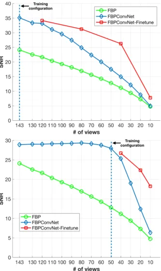
Fig. 9. Reconstruction quality vs number of views for training on 143 (upper graph) and 50 (bottom graph) projection views. ‘Training configuration’ is the number of projection views used during training. ‘Finetune’ means re-training with fewer projection views after first training with the original configuration.

lower here because of the relatively low contrast of the sinogram. In Fig. 7, we observe the same trend as for the biomedical dataset, where the TV method oversmooths and the FBPConvNet better preserves fine structures. These trends also appears in the twenty times downsampling case in Fig. 8. The FBPConvNet had a higher SNR than the TV method in both settings.

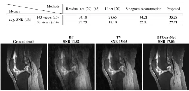
D. Comparison With Previous CNNs

Recently, many different CNN architectures have been pro-posed for segmentation [20] and regression problems [29], [63], [64]. In order to evaluate the effect of the choice of the network architecture on the reconstruction performance, the biomedical dataset was tested on two additional architec-tures: the residual net [29], [63] and the unmodified U-net [20]. We also applied our network to sinogram reconstruction prior to FBP reconstruction, similar to [64]. This comparison helps demonstrate the individual contributions of the elements of the CNN design discussed in Section III-B. For example, the residual net corresponds a residual network without

multireso-Fig. 10. The graph of SNR of reconstructed results vs testing sinogram noise level.

lution analysis, and, on the other hand, the conventional U-net has multiresolution without residual connections.

For this comparison, because of memory limitations, we reduced the number of angles for the full sinogram to 721 views. For all simulations, we did whole image processing which is different from the patch-based processing in [29], [64]. Table IV shows the results of experiment. From this table, we can conclude that the proposed method achieved the most robust reconstruction compared with other architectures and that it is better to use the FBP as pre-processing rather than to apply the CNN in the sinogram domain.

E. Stability

In this section, the stability of the proposed method is demonstrated in terms of the presence of additive white Gaussian noise (AGWN) and reduction of views in the testing set.

In one experiment, we trained the network on data with a fixed number of views, but varied the number of views in the testing data. The upper graph in Fig. 9 showed the degradation of SNR along with reducing number of views when the network was trained on 143 projection views. The red line comes from a fine-tuned network which was first trained from 143 views, and then trained for an additional 10 epochs with data using the new number of views (corresponding to 1.5 hours of training). The bottom graph in Fig. 9 shows a similar experiment for 50 views. The results show that testing in conditions different from training does degrade the performance of the network, but it is still significantly better than FBP reconstruction alone. Fine-tuning on data with the new conditions reduces this degradation.

In a second experiment, we trained the network on data with 50 or 143 projection views without additive white Gaussian noise. The graph in Fig. 10 shows stable performance as the SNR of the testing sinogram decreases: the reconstruction performance does not decrease until the SNR of the sinogram drops below 50 dB. At higher levels of noise, the performance

(11)

TABLE IV

COMPARISON OFSNR BETWEENDIFFERENTARCHITECTURES FORBIOMEDICALDATASET

Fig. 11. Ground truth image and reconstructed images of human knee dataset [65] from 6-fold downsampling in MRI using zero inserted inverse Fourier transform (‘BP’), TV regularized convex optimization [8] (channel by channel processing) (‘TV’), and the BPConvNet. (We use the term “BPConvNet” rather than “FBPConvNet” because, for MRI, there is no filtering required for direct inversion.)

of network gradually declines. From these analysis, we can observe that, although the network is trained on a specific configuration, the acceptable range of input is broader than original training conditions.

VI. DISCUSSION

The experiments provide strong evidence for the feasibility of the FBPConvNet for sparse-view CT reconstruction. The conventional iterative algorithm with TV regularization out-performed the FBPConvNet in the ellipsoidal dataset, while the reverse was true for the biomedical and experimental datasets. In these more-realistic datasets, the SNR improve-ment of the FBPConvNet came from its ability to preserve fine details in the images. This points to one advantage of the proposed method over iterative methods: the iterative methods must explicitly impose regularization, while the FBPConvNet effectively learns a regularizer from the data.

The computation time for the FBPConvNet was about 200 ms for the FBP and 200∼300 ms in GPU for the CNN for a 512×512 image. This is much faster than the iterative reconstruction, which, in our case, requires around 7 minutes even after the regularization parameters have been selected.

A major limitation of the proposed method is lack of transfer between datasets. For instance, when we put FBP images from a twenty-times subsampled sinogram into the network trained on the seven-times subsampled sinogram, the results retain many artifacts. Handling datasets of different dimensions or subsampling factors requires retraining the net-work. Future work could address strategies for heterogeneous datasets.

Our theory suggests that the methodology proposed here is applicable to all problems where the normal operator is shift-invariant; but, in the current work, we have presented and validated only a CNN specifically tailored for CT reconstruc-tion. There are important practical challenges in generalizing

the method to new modalites: Training the CNN requires a large set of training data (either from a high-quality forward model or real data), and a high-quality iterative reconstruc-tion algorithm is required for comparison. Further, while the presented theory works for complex-valued measurement operators, it is not straightforward to extend the current CNN architecture to complex-valued images. Any potential solution to this problem (e.g., using the modulus, or splitting the real and imaginary parts into different channels) requires experimental validation.

As a proof-of-concept of the generality of the method, we applied our network on accelerated MRI reconstruc-tion (Fig. 11). The experiment provides preliminary evidence for the feasibility of the FBPConvNet for accelerated MRI. For subsampling in MRI, we chose a variable density down-sampling mask with a factor of six in Fourier domain, and we made distorted images using this Fourier mask retrospectively. In order to handle complex values in the spatial domain, we took a modulus for each pixel in both input and output. We used 477 images for training and 25 for testing. The network architecture was the same as for the FBPConvNet for CT reconstruction. In accelerated MRI, FBPConvNet spent 100∼150 ms in the GPU for the CNN for a 320×320×8 volume (X×Y ×Ch multichannel images from [65]).

We also note that our theory predicts that certain modalities, such as structured-illumination microscopy (SIM), should not be amenable to reconstruction via the our method; this also requires experimental validation.

VII. CONCLUSION

In this paper, we proposed a deep convolutional network for inverse problems with a focus on biomedical imaging. The proposed method, which we call the FBPConvNet, combines FBP with a multiresolution CNN. The structure of the CNN is based on U-net, with the addition of residual learning.

(12)

This approach was motivated by the convolutional structure of several biomedical inverse problems, including CT, MRI, and DT. Specifically, we showed conditions on a linear oper-ator that ensure that its normal operoper-ator is a convolution. This results suggests that CNNs are well-suited to this subclass of inverse problems.

The proposed method demonstrated compelling results on synthetic and real data. It compared favorably to state-of-the-art iterative reconstruction on the two more realistic datasets. Furthermore, after training, the computation time of the pro-posed network per one image is under a second.

APPENDIX

For demonstration of actual implementations, we attach pseudo-code form of FBPConvNet (see Algorithm 1). Here, the most parameters (i.e. convolutional weights, biases, input, and output, etc.) are consistent with the notations in Fig.1 and Section III.

Algorithm 1 Forward Path of L-Level FBPConvNet

ACKNOWLEDGMENT

The authors would like to thank Dr. Cynthia McCollough, the Mayo Clinic, the American Association of Physicists in Medicine, and the National Institute of Biomedical Imaging and Bioengineering for giving us the opportunity to use real-in vivo CT DICOM images (Figs. 5 and 6). They would like to thank Dr. Marco Stampanoni, Swiss Light Source, Paul Scherrer Institute, Villigen, Switzerland, for providing real CT sinograms (Figs. 7 and 8). They would also like to thank the support of NVIDIA Corporation with the donation of the TITAN X GPU used for this research (especially for Table IV, and Figs. 9 and 10).

REFERENCES

[1] L. I. Rudin, S. Osher, and E. Fatemi, “Nonlinear total variation based noise removal algorithms,” Phys. D, Nonlinear Phenomena, vol. 60, nos. 1–4, pp. 259–268, 1992.

[2] A. Chambolle, “An algorithm for total variation minimization and applications,” J. Math. Imag. Vis., vol. 20, no. 1, pp. 89–97, 2004. [3] S. G. Chang, B. Yu, and M. Vetterli, “Adaptive wavelet thresholding for

image denoising and compression,” IEEE Trans. Image Process., vol. 9, no. 9, pp. 1532–1546, Sep. 2000.

[4] T. F. Chan and C.-K. Wong, “Total variation blind deconvolution,” IEEE Trans. Image Process., vol. 7, no. 3, pp. 370–375, Mar. 1998. [5] D. Krishnan and R. Fergus, “Fast image deconvolution using

hyper-Laplacian priors,” in Proc. Adv. Neural Inf. Process. Syst., 2009, pp. 1033–1041.

[6] M. Bertalmio, G. Sapiro, V. Caselles, and C. Ballester, “Image inpaint-ing,” in Proc. 27th Annu. Conf. Comput. Graph. Interactive Tech., 2000, pp. 417–424.

[7] E. J. Candès, J. Romberg, and T. Tao, “Robust uncertainty principles: Exact signal reconstruction from highly incomplete frequency informa-tion,” IEEE Trans. Inf. Theory, vol. 52, no. 2, pp. 489–509, Feb. 2006. [8] T. Goldstein and S. Osher, “The split Bregman method for L1-regularized problems,” SIAM J. Imag. Sci., vol. 2, no. 2, pp. 323–343, 2009.

[9] M. Lustig, D. Donoho, and J. M. Pauly, “Sparse MRI: The application of compressed sensing for rapid MR imaging,” Magn. Reson. Med., vol. 58, no. 6, pp. 1182–1195, 2007.

[10] H. Jung, K. Sung, K. S. Nayak, E. Y. Kim, and J. C. Ye, “k-t FOCUSS: A general compressed sensing framework for high resolution dynamic MRI,” Magn. Reson. Med., vol. 61, no. 1, pp. 103–116, 2009. [11] M. Guerquin-Kern, M. Häberlin, K. P. Pruessmann, and M. Unser,

“A fast wavelet-based reconstruction method for magnetic resonance imaging,” IEEE Trans. Med. Imag., vol. 30, no. 9, pp. 1649–1660, Sep. 2011.

[12] E. Y. Sidky and X. Pan, “Image reconstruction in circular cone-beam computed tomography by constrained, total-variation minimization,” Phys. Med. Biol., vol. 53, no. 17, p. 4777, Sep. 2008.

[13] M. G. McGaffin and J. A. Fessler, “Alternating dual updates algorithm for X-ray CT reconstruction on the GPU,” IEEE Trans. Comput. Imag., vol. 1, no. 3, pp. 186–199, Sep. 2015.

[14] M. T. McCann, M. Nilchian, M. Stampanoni, and M. Unser, “Fast 3D reconstruction method for differential phase contrast X-ray CT,” Opt. Exp., vol. 24, no. 13, pp. 14564–14581, Jun. 2016.

[15] Y. LeCun, Y. Bengio, and G. Hinton, “Deep learning,” Nature, vol. 521, pp. 436–444, May 2015.

[16] A. Krizhevsky, I. Sutskever, and G. E. Hinton, “ImageNet classification with deep convolutional neural networks,” in Proc. Adv. Neural Inf. Process. Syst., 2012, pp. 1097–1105.

[17] O. Russakovsky et al., “ImageNet large scale visual recognition challenge,” Int. J. Comput. Vis., vol. 115, no. 3, pp. 211–252, Dec. 2015.

[18] R. Girshick, J. Donahue, T. Darrell, and J. Malik, “Rich feature hierarchies for accurate object detection and semantic segmentation,” in Proc. IEEE Conf. Comput. Vis. Pattern Recognit., Jun. 2014, pp. 580–587.

[19] J. Long, E. Shelhamer, and T. Darrell, “Fully convolutional networks for semantic segmentation,” in Proc. IEEE Conf. Comput. Vis. Pattern Recognit., Jun. 2015, pp. 3431–3440.

[20] O. Ronneberger, P. Fischer, and T. Brox, “U-Net: Convolu-tional networks for biomedical image segmentation,” in Proc. Int. Conf. Med. Image Comput. Comput.-Assist. Intervent, 2015, pp. 234–241.

[21] H. C. Burger, C. J. Schuler, and S. Harmeling, “Image denoising: Can plain neural networks compete with BM3D?” in Proc. IEEE Conf. Comput. Vis. Pattern Recognit. (CVPR), Jun. 2012, pp. 2392–2399. [22] J. Xie, L. Xu, and E. Chen, “Image denoising and inpainting with

deep neural networks,” in Proc. Adv. Neural Inf. Process. Syst., 2012, pp. 341–349.

[23] L. Xu, J. S. Ren, C. Liu, and J. Jia, “Deep convolutional neural network for image deconvolution,” in Proc. Adv. Neural Inf. Process. Syst., 2014, pp. 1790–1798.

[24] C. Dong, Y. Deng, C. Change Loy, and X. Tang, “Compression artifacts reduction by a deep convolutional network,” in Proc. IEEE Int. Conf. Comput. Vis., Dec. 2015, pp. 576–584.

[25] J. Guo and H. Chao, “Building dual-domain representations for com-pression artifacts reduction,” in Proc. Eur. Conf. Comput. Vis., 2016, pp. 628–644.

(13)

[26] K. Kulkarni, S. Lohit, P. Turaga, R. Kerviche, and A. Ashok, “Recon-Net: Non-iterative reconstruction of images from compressively sensed measurements,” in Proc. IEEE Conf. Comput. Vis. Pattern Recognit., Jan. 2016, pp. 449–458.

[27] V. Golkov, A. Dosovitskiy, J. I. Sperl, M. I. Menzel, M. Czisch, P. Sämann, T. Brox, and D. Cremers, “q-space deep learning: Twelve-fold shorter and model-free diffusion MRI scans,” IEEE Trans. Med. Imag., vol. 35, no. 5, pp. 1344–1351, May 2016.

[28] C. Dong, C. C. Loy, K. He, and X. Tang, “Image super-resolution using deep convolutional networks,” IEEE Trans. Pattern Anal. Mach. Intell., vol. 38, no. 2, pp. 295–307, Feb. 2015.

[29] J. Kim, J. K. Lee, and K. M. Lee, “Accurate image super-resolution using very deep convolutional networks,” in Proc. IEEE Conf. Comput. Vis. Pattern Recognit. (CVPR), Jun. 2016, pp. 1646–1654.

[30] G. Riegler, M. Rüther, and H. Bischof, “ATGV-Net: Accurate depth super-resolution,” in Proc. Eur. Conf. Comput. Vis., 2016, pp. 268–284. [31] K. Gregor and Y. LeCun, “Learning fast approximations of sparse coding,” in Proc. 27th Int. Conf. Mach. Learn. (ICML), 2010, pp. 399–406.

[32] Y. Chen, W. Yu, and T. Pock, “On learning optimized reaction diffusion processes for effective image restoration,” in Proc. IEEE Conf. Comput. Vis. Pattern Recognit., Jun. 2015, pp. 5261–5269.

[33] B. Xin, Y. Wang, W. Gao, and D. Wipf, “Maximal sparsity with deep networks?” in Proc. Adv. Neural Inf. Process. Syst., 2016, pp. 4340–4348.

[34] A. Barbu, “Training an active random field for real-time image denois-ing,” IEEE Trans. Image Process., vol. 18, no. 11, pp. 2451–2462, Nov. 2009.

[35] U. Schmidt and S. Roth, “Shrinkage fields for effective image restora-tion,” in Proc. IEEE Conf. Comput. Vis. Pattern Recognit., Jun. 2014, pp. 2774–2781.

[36] I. Daubechies, M. Defrise, and C. De Mol, “An iterative threshold-ing algorithm for linear inverse problems with a sparsity constraint,” Commun. Pure Appl. Math., vol. 57, no. 11, pp. 1413–1457, Nov. 2004. [37] U. S. Kamilov and H. Mansour, “Learning optimal nonlinearities for iterative thresholding algorithms,” IEEE Signal Process. Lett., vol. 23, no. 5, pp. 747–751, May 2016.

[38] K. P. Pruessmann, M. Weigner, M. B. Scheidegger, and P. Boesiger, “SENSE: Sensitivity encoding for fast MRI,” Magn. Reson. Med., vol. 42, no. 5, pp. 952–962, 1999.

[39] K. He, X. Zhang, S. Ren, and J. Sun, “Deep residual learning for image recognition,” in Proc. IEEE Conf. Comput. Vis. Pattern Recognit., Jun. 2016, pp. 770–778.

[40] A. Kak and M. Slaney, Principles of Computerized Tomographic Imag-ing. Philadelphia, PA, USA: Society Industrial Applied Mathematics, 2001.

[41] M. Beister, D. Kolditz, and W. A. Kalender, “Iterative reconstruction methods in X-ray CT,” Phys. Med., vol. 28, no. 2, pp. 94–108, Apr. 2012. [42] S. Y. Chun, Y. K. Dewaraja, and J. A. Fessler, “Alternating direction method of multiplier for tomography with nonlocal regularizers,” IEEE Trans. Med. Imag., vol. 33, no. 10, pp. 1960–1968, Oct. 2014. [43] Q. Xu, H. Yu, X. Mou, L. Zhang, J. Hsieh, and G. Wang, “Low-dose

X-ray CT reconstruction via dictionary learning,” IEEE Trans. Med. Imaging, vol. 31, no. 9, pp. 1682–1697, Sep. 2012.

[44] D. M. Pelt and K. J. Batenburg, “Fast tomographic reconstruction from limited data using artificial neural networks,” IEEE Trans. Image Process., vol. 22, no. 12, pp. 5238–5251, Dec. 2013.

[45] D. Boublil, M. Elad, J. Shtok, and M. Zibulevsky, “Spatially-adaptive reconstruction in computed tomography using neural networks,” IEEE Trans. Med. Imag., vol. 34, no. 7, pp. 1474–1485, Jul. 2015. [46] H. Chen, Y. Zhang, W. Zhang, P. Liao, K. Li, J. Zhou, and G. Wang,

“Low-dose CT via convolutional neural network,” Biomed. Opt. Exp., vol. 8, no. 2, pp. 679–694, Feb. 2017.

[47] Y. Han, J. Yoo, and J. C. Ye. “Deep residual learning for compressed sensing ct reconstruction via persistent homology analysis.” [Online]. Available: https://arxiv.org/abs/1611.06391, 2016.

[48] S. Horbelt, M. Liebling, and M. Unser, “Discretization of the radon transform and of its inverse by spline convolutions,” IEEE Trans. Med. Imag., vol. 21, no. 4, pp. 363–376, Apr. 2002.

[49] R. Tibshirani, “Regression shrinkage and selection via the LASSO,” J. Roy. Statist Soc. Ser. B (Methodol.), vol. 58, no. 1, pp. 267–288, 1996. [50] M. Elad, P. Milanfar, and R. Rubinstein, “Analysis versus synthesis in

signal priors,” Inverse problems, vol. 23, no. 3, p. 947, 2007. [51] A. L. da Cunha, J. Zhou, and M. N. Do, “The nonsubsampled

con-tourlet transform: Theory, design, and applications,” IEEE Trans. Image Process., vol. 15, no. 10, pp. 3089–3101, Oct. 2006.

[52] S. Mallat, A Wavelet Tour of Signal Processing. San Diego, CA, USA: Academic, 1999.

[53] R. R. Coifman and D. L. Donoho, Translation-Invariant De-Noising. New York, NY, USA: Springer, 1995.

[54] S. Boyd, N. Parikh, E. Chu, B. Peleato, and J. Eckstein, “Distributed optimization and statistical learning via the alternating direction method of multipliers,” Found. Trends Mach. Learn., vol. 3, no. 1, pp. 1–122, Jan. 2011.

[55] A. Beck and M. Teboulle, “A fast iterative shrinkage-thresholding algorithm for linear inverse problems,” SIAM J. Imag. Sci., vol. 2, no. 1, pp. 183–202, 2009.

[56] M. V. Afonso, J.-M. Bioucas-Dias, and M. A. T. Figueiredo, “Fast image recovery using variable splitting and constrained optimization,” IEEE Trans. Image Process., vol. 19, no. 9, pp. 2345–2356, Sep. 2010. [57] M. D. Zeiler and R. Fergus, “Visualizing and understanding

convolu-tional networks,” in Proc. Eur. Conf. Comput. Vis., 2014, pp. 818–833. [58] J. Cong and B. Xiao, “Minimizing computation in convolutional neural networks,” in Proc. Int. Conf. Artif. Neural Netw., 2014, pp. 281–290. [59] M. Rhu, N. Gimelshein, J. Clemons, A. Zulfiqar, and S. W. Keckler,

“vDNN: Virtualized deep neural networks for scalable, memory-efficient neural network design,” in Proc. 49th Annu. IEEE/ACM Int. Symp. Microarchitecture (MICRO), Oct. 2016, pp. 1–13.

[60] A. Vedaldi and K. Lenc, “Matconvnet: Convolutional neural networks for matlab,” in Proc. ACM Int. Conf. Multimedia, 2015, pp. 689–692. [61] R. Pascanu, T. Mikolov, and Y. Bengio, “On the difficulty of

training recurrent neural networks,” in Proc. ICML, vol. 28. 2013, pp. 1310–1318.

[62] M. Unser, J. Fageot, and H. Gupta, “Representer theorems for sparsity-promoting1regularization,” IEEE Trans. Inf. Theory, vol. 62, no. 9, pp. 5167–5180, Sep. 2016.

[63] K. Zhang, W. Zuo, Y. Chen, D. Meng, and L. Zhang, “Beyond a Gaussian Denoiser: Residual learning of deep CNN for image denois-ing,” IEEE Trans. Image Process., vol. 26, no. 7, pp. 3142–3155, Jul. 2017.

[64] H. Lee, J. Lee, and S. Cho, “View-interpolation of sparsely sampled sinogram using convolutional neural network,” Proc. SPIE, vol. 10133, p. 1013328, Feb. 2017.

[65] K. Epperson, A. M. Sawyer, M. Lustig, M. Alley, M. Uecker, P. Virtue, P. Lei, and S. Vasanawala, “Creation of fully sampled mr data repository for compressed sensing of the knee,” in Proc. SMRT Conf., 2013.

Kyong Hwan Jin received the B.S. and the

integrated M.S. and Ph.D. degrees from the Depart-ment of Bio and Brain Engineering, Korea Advanced Institute of Science and Technology (KAIST), Daejeon, South Korea, in 2008 and 2015, respec-tively. He was a Post-Doctoral Scholar with KAIST from 2015 to 2016. He is currently a Post-Doctoral Scholar with the Biomedical Imaging Group, École Polytechnique Fédérale de Lausanne, Switzerland. His research interests include low rank matrix com-pletion, sparsity promoted signal recovery, sampling theory, biomedical imaging, and image processing in various applications.

Michael T. McCann (S’10–M’15) received the

B.S.E. in biomedical engineering from the Univer-sity of Michigan in 2010 and the Ph.D. degree in biomedical engineering from Carnegie Mellon University in 2015. He is currently a Scientist with the Laboratoire d’Imagerie biomédicale and centre d’imagerie biomédicale, École Polytechnique Fédérale de Lausanne, where he is involved in X-ray CT reconstruction. His research interest cen-ters on developing signal processing tools to answer biomedical questions.

(14)

Emmanuel Froustey received the Dipl.Eng. degree

from CentraleSupélec, Châtenay-Malabry, France, in 2012, and the M.Sc. degree in computational science and engineering from the École Polytech-nique Fédérale de Lausanne, Lausanne, Switzerland, in 2014. He is currently a Research and Develop-ment Engineer with Dassault Aviation. His research interests include variational models and optimization algorithms with applications to biomedical imaging.

Michael Unser (M’89–SM’94–F’99) is currently a

Professor and the Director of École Polytechnique Fédérale de Lausanne’s Biomedical Imaging Group, Lausanne, Switzerland. From 1985 to 1997, he was with the Biomedical Engineering and Instrumenta-tion Program, NaInstrumenta-tional Institutes of Health, Bethesda USA, where he was involved in bioimaging. He has authored over 250 journal papers on those topics. He is the author with P. Tafti of the book An introduction to sparse stochastic processes (Cambridge Univer-sity Press 2014). His primary area of investigation is biomedical image processing. He is internationally recognized for his research contributions to sampling theory, wavelets, the use of splines for image processing, stochastic processes, and computational bioimaging. He is currently a member of the editorial boards of the SIAM Journal on Imaging Sciences, and Foundations and Trends in Signal Processing. He is also a fellow of EURASIP in 2009, and a member of the Swiss Academy of Engineering Sciences. He was a recipient of several international prizes including three IEEE-SPS Best Paper Awards and two Technical Achievement Awards from the IEEE (2008 SPS and EMBS 2010). He is also the founding Chair of the Technical Committee on Bio Imaging and Signal Processing of the IEEE Signal Processing Society. He has held the position of Associate Editor-in-Chief of the IEEE TRANSACTIONS ONMEDICALIMAGINGfrom 2003 to 2005.