8
in Dynamic Social Networks
YU-RU LINArizona State University
YUN CHI and SHENGHUO ZHU NEC Laboratories America HARI SUNDARAM
Arizona State University and
BELLE L. TSENG YAHOO! Inc.
We discover communities from social network data and analyze the community evolution. These communities are inherent characteristics of human interaction in online social networks, as well as paper citation networks. Also, communities may evolve over time, due to changes to individuals’ roles and social status in the network as well as changes to individuals’ research interests. We present an innovative algorithm that deviates from the traditional two-step approach to analyze community evolutions. In the traditional approach, communities are first detected for each time slice, and then compared to determine correspondences. We argue that this approach is inappropri-ate in applications with noisy data. In this paper, we proposeFacetNetfor analyzing communities and their evolutions through a robustunifiedprocess. This novel framework will discover communi-ties and capture their evolution with temporal smoothness given by historic community structures. Our approach relies on formulating the problem in terms of maximum a posteriori (MAP) estima-tion, where the community structure is estimated both by the observed networked data and by the prior distribution given by historic community structures. Then we develop an iterative algorithm, with proven low time complexity, which is guaranteed to converge to an optimal solution. We per-form extensive experimental studies, on both synthetic datasets and real datasets, to demonstrate that our method discovers meaningful communities and provides additional insights not directly obtainable from traditional methods.
Authors’ addresses: Y-R Lin and H. Sundaram, Arts, Media and Engineering Program, Arizona State University, Tempe, AZ 85281; Y. Chi and S. Zhu, NEC Labs America, 10080 N. Wolfe Rd, SW3-350, Cupertino, CA 95014. B. L. Tseng, YAHOO! Inc., 2821 Mission College Blvd, Santa Clara, CA 95054; email: [email protected].
Permission to make digital or hard copies of part or all of this work for personal or classroom use is granted without fee provided that copies are not made or distributed for profit or commercial advantage and that copies show this notice on the first page or initial screen of a display along with the full citation. Copyrights for components of this work owned by others than ACM must be honored. Abstracting with credit is permitted. To copy otherwise, to republish, to post on servers, to redistribute to lists, or to use any component of this work in other works requires prior specific permission and/or a fee. Permissions may be requested from Publications Dept., ACM, Inc., 2 Penn Plaza, Suite 701, New York, NY 10121-0701 USA, fax+1 (212) 869-0481, or [email protected].
C
2009 ACM 1556-4681/2009/04-ART8 $5.00
Categories and Subject Descriptors: H.2.8 [Database Management]: Database Applications—
Data mining; H.3.3 [Information Storage and Retrieval]: Information Search and Retrieval—
Information filtering; J.4 [Computer Applications]: Social and Behavioral Sciences—Economics
General Terms: Algorithms, Experimentation, Measurement, Theory
Additional Key Words and Phrases: Community, community net, evolution, evolution net, nonneg-ative matrix factorization, soft membership
ACM Reference Format:
Lin, Y.-R., Chi, Y., Zhu, S., Sundaram, H., and Tseng, B.L. 2009. Analyzing communities and their evolutions in dynamic social networks. ACM Trans. Knowl. Discov. Data. 3, 2, Article 8 (April 2009), 31 pages. DOI=10.1145/1514888.1514891 http://doi.acm.org/10.1145/1514888.1514891
1. INTRODUCTION
This article focuses on the development of a comprehensive framework to ana-lyze community evolution from online social networks. This is motivated by the central belief that semantics of information is an emergent artifact of human activity, and the relationship between semantic concepts and their manifesta-tions (i.e., Web pages, blog posts) evolves over time. Human networks have been the locus for the construction of meaning hence it is crucial to find real human networks that collaborate with respect to some activity.
Data from many social network datasets, including paper coauthorship net-works and the blogosphere, is a graph where nodes represent individuals (e.g., club members, authors, and bloggers) and edges represent the relationship and interactions among individuals (e.g., interactions in a club, coauthorship, and hyperlinks in blogs). In such social networks, individuals form communities by building relationships and interactions with each other. The analysis of these communities (membership, structure and temporal dynamics) is an important research issue.
Traditional analysis of social networks treats the network as as a static graph, where the static graph is either derived from aggregation of data over all time or taken as a snapshot of data at a particular time. These studies range from well-established social network analysis [Wasserman and Faust 1994] to recent successful applications such as HITS and PageRank [Kleinberg 1999; Page et al. 1998]. However, this research omits one important feature of communities in networked data—the temporal evolution of communities. By ignoring community evolution, prior works have overlooked a key aspect of online communities.
More recently, there has been a growing body of work on the analysis of communities and their temporal evolution in dynamic networks[Asur et al. 2007; Kumar et al. 2003; Kumar et al. 2006; Leskovec et al. 2005; Lin et al. 2007; Palla et al. 2007; Spiliopoulou et al. 2006; Toyoda and Kitsuregawa 2003]. How-ever, a common weakness in these studies, as we will discuss in detail in related work, is that communities and their evolutions are studied separately—usually, community structures are independently extracted at consecutive timesteps and then in retrospect, evolutionary characteristics are introduced to explain
the difference between these community structures over time. Such a two-stage approach may make sense when the community structure is unambiguous (e.g., when the community affiliation is available). However, more often than not, data from real-world networks are ambiguous and subject to noise. Under such scenarios, if an algorithm extracts community structure for each timestep in-dependently of other timesteps, it often results in community structures with high temporal variation. Consequently, undesirable evolutionary characteris-tics may have to be introduced in order to explain the high variation in the community structures. Therefore, we argue that a more appropriate approach is to analyze communities and their evolutions in a unified framework where the community structure provides evidence about community evolutions and at the same time, the evolutionary history offers hints on what community struc-ture is more appropriate. For example, a community strucstruc-ture that introduces dramatic evolutions in a very short period of time is less desirable.
Another common problematic issue in current community analysis tech-niques is that an individual is usually assigned to only one community at a time. On the contrary, an individual may be engaged in multiple communities at the same time. For example, a blogger who is a dance guru may also be an amateur photographer at the same time. Because of this, an individual who usually participates in multiple communities should be assigned to multiple communities at the same time. Therefore, instead of a hard community par-tition, we argue that a soft community membership is more informative, as it provides more details about how an individual participates in each of the communities.
In this paper, we propose a systematic framework for analyzing communi-ties and their evolutions in dynamic networks, and we term our framework FacetNet.1Our main contributions are threefold:
1. We introduce the FacetNet framework to analyze communities and their evolutions in a unified process. In our framework, the community structure at a given timestep t is determined both by the observed networked data at t and by the prior distribution given by historic community structures. Algorithmically, we propose the first probabilistic generative model for an-alyzing communities and their evolution. We show that the proposed model solves the evolutionary clustering problem from a probabilistic (Bayesian) perspective. Empirically, the discovered communities and their evolutions are more robust to noise and more reasonable (e.g., dramatic change in a short time is unlikely).
2. We adopt a stochastic block model for generating communities and a probabilistic model based on the Dirichlet distribution for capturing the com-munity evolutions. These probabilistic models naturally assign soft commu-nity memberships to nodes and these models do not suffer from the problem of non-identifiability of parameters which exists in most existing models. Based on the probability distributions computed by the models, we further 1FacetNet stands for “a Framework for Analyzing Communities and EvoluTions in dynamic
introduce two novel concepts—Community NetandEvolution Net—to inter-pret the community-level interaction and transition, respectively.
3. We provide an iterative EM algorithm that is guaranteed to converge to op-timal solutions to the proposed formulation. We prove the correctness and convergence of our algorithm and show that this algorithm has low time complexity when the data is sparse. We also provide principled solutions to some practical issues, such as how to determine the number of communi-ties and how to handle adding and removing of individuals in a dynamic network.
We use synthetic and real datasets (including a blog dataset and a paper coauthorship dataset) to demonstrate that compared to traditional methods, our framework provides more accurate and robust results on communities and their evolutions. We also show that our framework is able to discover interesting insights in dynamic networks that are not directly obtainable from existing methods.
This article is a significant extension of our prior work [Lin et al. 2008] and is our first comprehensive discussion on this subject. In this article, we include new theoretical and experimental results as well as detailed algorithms and proofs. In particular there are several major extensions over prior work [Lin et al. 2008].
1. An extension of the theoretical framework: We present a theoretically motivated and more generalized framework in this article. We reformulate the problem in terms of maximum a posteriori (MAP) estimation and show a close connection between the proposed generative probabilistic model and the optimization framework for solving the evolutionary clustering problem (Section 2).
2. Details of the algorithms: We provide an EM algorithm for solving the MAP problem and provide the proof of the convergence of this algorithm (Sec-tion 4). In addi(Sec-tion, we provide an algorithm with proof of correctness for solving the extended MAP problem where the number of communities is allowed to change over time (Section 5).
3. New and extensive experiment results: In the experiment on synthetic datasets, we compare our algorithm with three baseline algorithms in terms of a graph based error rate measure. We provide a new comparison against the variability of the ground truth community structures and show a signif-icant performance improvement of our algorithm (Section 6) in this aspect. Moreover, we provide more experimental results from a real world paper citation dataset. These concrete findings suggest the applicability of our al-gorithm to the large scale social networks (Section 6).
The rest of the article is organized at follows. First, we discuss related work. In Section 2, we present the formulation of our model in detail. In Section 3, we describe how to extract communities and their evolutions from the results learn by our probabilistic model. In Section 4, we propose an iterative EM algorithm for solving our model and discuss the time complexity of the proposed algorithm. In Section 5, we introduce extensions of our framework to handle some practical
issues. In Section 6, we provide experimental studies. Finally in Section 7, we give the conclusion and future directions.
1.1 Related Work
Community formation has been extensively studied in various research areas such as social network analysis, Web community analysis, computer vision, etc. In social network analysis, an important research topic is to identify co-hesive subgroups of individuals within a network where coco-hesive subgroups are defined as “subsets of actors among whom there are relatively strong, di-rect, intense, frequent, or positive ties” [Wasserman and Faust 1994]. Many approaches, such as clique-based, degree-based, and matrix-perturbation-based, have been proposed to extract cohesive subgroups from social network [Wasserman and Faust 1994].Communities also play an important role in Web analysis. For example, Flake et al. [2000] defined Web communities as “a set of sites that have more links to members of the community than to non-members,” and proposed algorithms to identify Web communities based on a maximum flow/minmum cut framework. Newman and Girvan [2004] defined a metric called modularity measure to quantify the strength of community structure and they also proposed several community extraction algorithms by using this modularity measure. We will discuss the details about modularity in a later section. In computer vision, community extraction is closely related to image segmentation problem, which is a problem to partition an image into multiple regions so that pixels within the same region are similar and adjacent regions are significantly different. One effective method in this area is the spectral clustering algorithm [Chung 1997; Dhillon et al. 2004; Shi and Malik 2000; Zha et al. 2001] where the eigenvectors of certain normalized similarity matri-ces are used for the clustering purpose. Later, White and Smyth [2005] pointed out the close relationship between Newman’s modularity and the spectral clus-tering and proposed several algorithms to combine the two approaches. Yu et al. [2005] proposed a novel clustering framework on graphs where the cluster berships are assigned in a probabilistic way. In Yu’s framework, cluster mem-berships can be extracted in different resolutions, representing local or global cluster structures. A common issue in all the above studies is that they only an-alyzedstatic networkswhere no temporal analysis is used for evolution study. Another issue is that most of these studies treat community extraction as a graph partition problem and therefore always result in hard community mem-berships, which disallows an individual to participate multiple communities at the same time.
Recently, there exists a growing body of literature on analyzing communities and their evolutions indynamic networks. Kumar et al. [2003] studied the evo-lution of the blogosphere as a graph in terms of the change of characteristics, (such as in-degree, out-degree, strongly connected components), the change of communities, as well as the burstiness in blog community.Leskovec et al. [2005] studied the patterns of growth for graphs in various fields and proposed gen-erators that produce graphs exhibiting the discovered patterns. Palla et al. [2007] analyzed a coauthorship network and a mobile phone network, where
both networks are dynamic. They use the clique percolation method (CPM) to extract communities at each timestep and then match communities in consecu-tive timesteps to analyze community evolution. They studied some interesting characteristics, such as community sizes, ages and their correlation, community autocorrelation (relative overlap between the same community at two timesteps t1andt2as a function ofτ =t2−t1), etc. Toyoda and Kitsuregawa [2003] studied the evolution of Web communities from a series of Web achieves. They first pro-posed algorithms for extracting communities in each timestep. And then they proposed different types of community changes, such as emerge, dissolve, grow, and shrink, as well as a set of metrics to quantify such changes for community evolution analysis. Spiliopoulou et al. [2006] proposed a framework, MONIC, to model and monitor cluster transitions over time. They defined a set of exter-nal transitionssuch as survive, split, disappear, to model transactions among different clusters and a set of internal transitions, such as size and location transitions to model changes within a community. Asur et al. [2007] introduced a family of events on both communities and individuals to characterize evo-lution of communities. Sun et al. [2007] proposed a parameter-free algorithm, GraphScope, to mine time-evolving graphs where the Minimum Description Length (MDL) principle is employed to extract communities and to detect com-munity changes. Mei and Zhai [2005] extracted latent themes from text and used the evolution graph of themes for temporal text mining. All these studies, however, have a common weak point—community extraction and community evolution are analyzed in two separated stages. That is, when communities are extracted at a given timestep, historic community structure, which contains valuable information related to current community structure, is not taken into account.
There are some recent studies on evolutionary embedding and clustering that are closely related to our work. Sarkar and Moore [2005] proposed a dy-namic method that embeds nodes into latent spaces where the locations of the nodes at consecutive timesteps are regularized so that dramatic change is unlikely. Chakrabarti et al. [2006] proposed the first evolutionary clus-tering methods where the cluster membership at time t is influenced by the clusters at time t-1. As a result, the cluster membership for a node at time t depends both on its relationship with other nodes at time t and on its cluster membership at time t-1. Chi et al. [2007] extended similar ideas and proposed the first evolutionary spectral clustering algorithms. They used graph cut as a metric for measuring community structures and community evolutions.
All these studies differ from our work in that they regularize the current community membership at timetby using historic community membership in-directly. In Chakrabarti et al.’s evolutionary hierarchical clustering algorithm, historic community structure affects the tree-node merging step in the current time. In their evolutionaryk-means clustering algorithm, historic centroids af-fect thek-mean process at the current time. In Chi et al.’s algorithms, certain eigenvectors, instead of the community structure, are regularized over time. In the work of Sarkar et al., although the relationship among nodes in la-tent spaces is preserved over time, the issue of communities are not directly
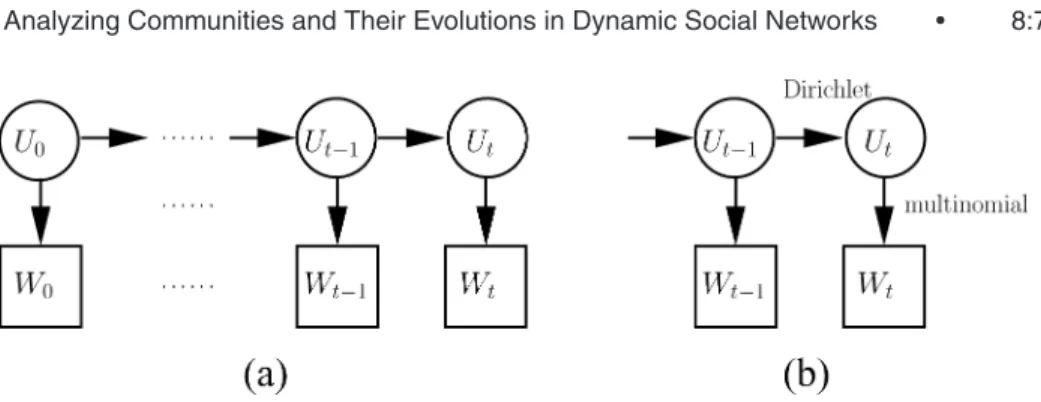
Fig. 1. Schematic illustrations of (a) our high-level abstract probabilistic model and (b) one in-stance of the concrete probabilistic model.
addressed. In contrast, in our proposed framework, the community membership itself is directly regularized over time.
2. FORMULATION 2.1 Notation
First, a note on notation. In this paper, we use lower-case letters, for example, x, to represent scalars, vector-formed letters, e.g.,v, to represent vectors, and upper-case letters, for example,W, to represent matrices. Bothwij and (W)ij represent the element at thei-th row and j-th column ofW. We use vec (W) to denote the vectorization ofW, that is, stacking the columns ofW into a column vector. A subscriptt on a variable, for example, Wtorwt;i j, denotes the value of that variable at timet. However, to avoid notation clutter, we try not to use the subscripttunless it is needed for clarity.
We assume that edges in the networked data are associated with discrete timesteps. We use asnapshotgraphGt(Vt,Et,Wt) to model interactions at time t where in Gt, each node vi ∈ Vt represents an individual, each edgeeij ∈ Et represents the presence of interactions between vi and vj, and wt;i j = (Wt)ij denotes the edge weight ofeij(i.e., the frequency of interactions between nodes iand j observed at timet). AssumingGthasnnodes,Wt∈Rn+×n(nonnegative matrix of sizen×n) is the adjacency matrix forGt. Over time, the interaction history is captured by a sequence of snapshot graphsG1,· · · ,Gt,· · · indexed by time.
2.2 Basic Formulation
We start by introducing our probabilistic generative model that describes com-munities and their evolutions. The basic principles behind our models are (1) the data observed at timet (i.e., Wt) is generated from the community struc-ture at timet(the structure parameter set is denoted byUt), following a certain distribution, and (2) the community structureUtfollows a certain distribution that is determined by the community structureUt−1at timet-1. Furthermore, we assume thatWtis independent ofUt−1givenUt, as illustrated in Figure 1(a). We estimate the parameters{Ut}using maximum a posteriori (MAP) esti-mation. For simplicity, in this paper we only discuss the forward estimation,
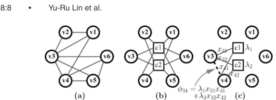
Fig. 2. Schematic illustration of the stochastic block model: (a) the original graph, (b) the bipartite graph with two communities, and (c) how to approximate (φ34).
that is, assuming thatUt−1is given when estimatingUt. Mathematically, we write
Ut∗ =arg max U
logP(Wt|U)P(U|Ut−1). Equivalently, we want to maximize the following
L(Ut)=logP(Wt|Ut)+logP(Ut|Ut−1). (1) Therefore, our high-level abstract model contains two components— P(Wt|Ut) and P(Ut|Ut−1)—and these components can be defined in different ways to give different concrete models. In the following sections, we present some concrete models for P(Wt|Ut) andP(Ut|Ut−1).
2.3 The Model forP(Wt|Ut)
For P(Wt|Ut), we adopt a stochastic block model first proposed in Yu et al. [2005]. Assume there existmcommunities at timet and thesemcommunities introduce a probabilityφt;i j for the interaction between nodesiand j by using a mixture model. In the mixture model, φt;i j =
m
k=1pk· pk→i · pk→j, where pk is the prior probability that the interaction between nodesi and j is due to thek-th community,pk→iand pk→j are the probabilities that an interaction in community k involves node vi and vj, respectively. We explicitly write a parameter setUt, as a nonnegative matrixXt∈Rn+×mand anm×mnonnegative diagonal matrixt, wherext;ik = pk→i,λt;k = pk,
ixt;ik =1 and
kλt;k =1, (λt;kis short forλt;kk). Thus, we haveφt;i j =(XttXTt )ij. An alternative model is that{φt;i j}is generated by a bipartite graph where nodes on one side of the graph represent the originalnnodes inWtand those on the other side represent them communities. In Figure 2, we use a toy example with 6 nodes and 2 communities to illustrate this model of community structure. For a general graph (a), we use a special bipartite graph (b) to approximate (a). Note that (b) has two more nodesc1andc2, corresponding to the two communities. Nevertheless, because (b) is a bipartite graph (i.e., an edge can only occur between a node vand a community c), it has less degree of freedom and so it is a more parsimonious explanation of (a). In (c), we show how the probabilityφ34is generated in the mixture model as the sum ofλ1x31x41andλ2x32x42.
Matrices Xt andt fully characterize this mixture model and therefore we defineUt =(Xt,t). We then model P(Wt|Ut) by a multinomial distribution
with parameterφt;i j, which results in logP(Wt|Ut)=log(1+ ijwt;i j) ij(1+wt;i j) ij φwt;i j t;i j = ij wt;i jlogφt;i j +const,
where(·) is the gamma function. 2.4 The Model forP(Ut|Ut-1)
Because the columns of Xt all sum to ones and t is a diagonal matrix, Xtt can uniquely determine Xt and t. Therefore, we have P(Ut|Ut−1) =
P(Xtt|Xt−1t−1). Since we use the multinomial distribution to model
P(Wt|Ut) and since the conjugate prior for the multinomial distribution is the Dirichlet distribution, it is a natural choice to use a Dirichlet distribution as the prior distribution. We let vec (Xtt) follow a Dirichlet distribution with pa-rameterψt =ν·vec (Xt−1t−1)+ 1. Through the parameterψt, the distribution P(Ut) of the community structure at timet is determined by the community structureUt−1at timet-1. Under this model, we have
logP(Ut|Ut−1)=log (jψt;j) j(ψt;j) ik (Xtt)ikν·(Xt−1t−1)ik = ik ν·(Xt−1t−1)iklog (Xtt)ik+const.
The parameterνcan be set by the user. We will discuss the role ofνin the next section.
2.5 The Overall Model and Its Connection to Evolutionary Clustering PuttingP(Wt|Ut) and P(Ut|Ut−1) together, we have
L(Ut)=logP(Wt|Ut)+logP(Ut|Ut−1) = ij (Wt)ijlog XttXtT ij+ ik ν·(Xt−1t−1)iklog(Xtt)ik+const. (2)
Figure 1(b) illustrates the overall concrete model that we propose.
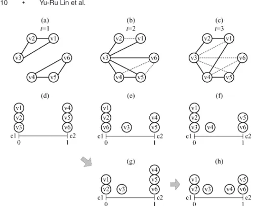
The effect of P(Ut|Ut−1) is illustrated by using a toy example in Figure 3. Figure 3(a)–(c) show the interactions among the six nodes occurring at time t = 1, 2 and 3, where the blue solid lines represent the new observed inter-actions at each time and the gray dotted lines are the interinter-actions observed previously. Figure 3(d)–(f) show the community membership resulted from each observed snapshot alone (i.e. without considering the historic interactions). The horizontal axis indicates the probabilities of a nodevi belonging to the commu-nityc1 orc2, for example, a node lies at 1 means it belongs toc2 with probability 1 and belongs toc1 with probability 0. We can simply assign the membership to a node based on the probability value. As can be seen, the community struc-ture att=1 is obvious. Att = 2, the interactions betweenv3 and every other nodes makev3’s membership ambiguous, and this ambiguity suddenly changes
Fig. 3. A toy example for illustrating the evolutionary stochastic block model. (a)–(c): The interac-tions among the six nodes occurring at timet=1, 2 and 3. (At each time, blue solid lines represent new observed interactions and gray dotted lines represent previously observed interactions.) (d)–(f): The community membership resulted from each observed snapshot. The resultant abrupt mem-bership fails to capture meaningful community evolution. (g)–(h): The community memmem-bership resulted from both the new observation and the historic community structures. The horizontal axis in (d)–(h) indicates the probabilities of a nodevibelonging to the communityc1 orc2. Our model
gives more desirable results. By considering the historic community structure in (d), the member-ship ofv3 att=2 is more discriminate in (g) than in (e), andv3’s interactions with everyone does not affect others’ membership significantly.
v6’s membership (Figure 3(e)). The abrupt membership assignment can also be noticed at t = 3 (v3, v4 and v6). Such results are undesirable because they fail to capture meaningful community evolution. Under our model, both the new observation and the historic community structures (Figure 3(d) and (g)) are considered, which results in different membership assignment as shown in Figure 3(g) and (h). The results are close to our intuition: given we already observe data at t = 1, the membership of v3 at t = 2 is more discriminate, and v3’s undiscriminate interactions with everyone should not affect others’ membership significantly.
It turns out that the model described by Equation (2) has a close connection to the evolutionary clustering framework ([Chakrabarti et al. 2006; Chi et al. 2007]). In evolutionary clustering, communities and their evolutions influence each other. That is, at timet, a community structure is preferred if the commu-nity evolution fromt-1totis not unreasonably dramatic. To achieve this goal, the community structure at time t-1(already extracted) is used to regularize the community structure at current timet(to be extracted). To incorporate such
a regulation, a cost function is introduced to measure the quality of community structure at timet, where the cost consists of two parts—asnapshot costand a temporal cost:
cost=α·CS+(1−α)·CT. (3) In this cost function, the snapshot costCSmeasures how well a community structure fits Wt, the observed interactions at time t. The temporal cost CT measures how consistent the community structure is with respect to historic community structure (at timet-1). The parameterαis set by the user to control the level of emphasis on each part of the total cost.
To see the connection between our probabilistic generative model and that in evolutionary clustering, we define the snapshot costCSas the following. By using a bipartite graph as before, we approximateWt, which has rankn, by a product in the form of XttXtT, which has rank m. Based on this model, we define the snapshot costCSas the error introduced by such an approximation, that is,
CS=DWt XttXtT
,
whereD(A B)=i,j(ai jlogai jbi j−ai j+bi j) is the KL-divergence betweenAand B. So the snapshot cost is high when the approximate community structure XttXTt fails to fit the observed dataWtwell.
The temporal costCT is used to regularize the community structure so that it is less probable for unreasonably dramatic community evolution from time t-1to t. We can achieve this regularization by defining CT as the difference between the community structure at timet and that at timet-1; that is,
CT =D(Xt−1t−1 Xtt),
whereDis the KL-divergence as defined before. So the temporal costCT is high when there is a dramatic change of community structure from timet-1tot.
Putting the snapshot costCS and the temporal cost CT together, we have an optimization problem as to find the best community structure at time t, expressed byXt andt, that minimizes the following total cost
cost=α·D(Wt XttXTt )+(1−α)·D(Xt−1t−1 Xtt) (4) subject toXt ∈Rn+×m,ixt;ik=1, andtbeing anm-by-mnonnegative diago-nal matrix.
The connection between our probabilistic generative model and the evolu-tionary clustering problem formulated in Equation (4) is the following: min-imizing Equation (4) turns out to be equivalent to maxmin-imizing Equation (2) under certain conditions, as described in the following theorem. We provide the proof in the appendix.
THEOREM 2.1. Under the assumption thatij(Wt)ijremains a constant over time (i.e., the number of observed interactions in all timesteps are the same), minimizing the cost in Eq. (4) is equivalent to minimizing the logarithm in Eq.(2)withν=(1−α)/α.
It is worth mentioning that although Equation (4) shares a similar form to that of evolutionary spectral clustering [Chi et al. 2007], it has a good prop-erty that is not in evolutionary spectral clustering. In evolutionary spectral clustering, the parameters learned are eigenvalues and eigenvectors and as a result, a second step ofk-means clustering is needed to determine the final clus-ter memberships. With such a second step, in addition to being nonintuitive, evolutionary spectral clustering suffers from a problem of nonidentifiability of parameters. That is, the clusters at timet-1are not explicitly mapped to those clusters at time t and therefore some partition-matching algorithms [Lovasz and Plummer 1986] must be used to obtained the optimal cluster mapping be-tween those at timet-1and those at timet, where the partition-matching is an NP-hard problem. Equation (4), in contrast to evolutionary spectral clus-tering, has the property that X and are nonnegative. The benefit of this nonnegativity is that the resulting Xat each timestepdirectlyindicates the cluster memberships (as a probabilistic distribution). As a result, the problem of nonidentifiability of parameters is usually not an issue: because of the regular-ization termD(Xt−1t−1 Xtt), the algorithm usually converges to a solution with the optimal mapping between the clusters at timet-1and those at timet automatically chosen.
3. EXTRACTING COMMUNITIES AND THEIR EVOLUTIONS
After obtaining the solutionUt for all timesteps, here are the ways we utilize the solution to analyze communities and their evolutions.
3.1 Community Membership
Assume we have computed the result at timet-1, that is, (Xt−1,t−1), and the result at time t, that is, (Xt,t). In addition, we define a diagonal matrix Dt, whose diagonal elements are the row sums ofXtt, that is,dt;ii =
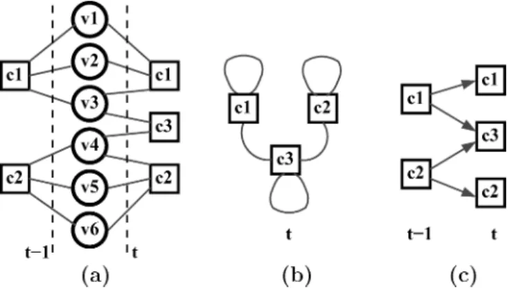
j(Xtt)ij. Then we can see that the i-th row of D−t1Xtt indicates the soft community memberships of vi at time t. We illustrate this by using an example shown in Figure 4. Recall that in the bipartite graph at time t (the right side of Figure 4(a)), the weights of edges connecting vi to c1,c2, andc3represent the joint probability P(vi,c1),P(vi,c2), and P(vi,c3). TheDt−1part normalizes this joint probability to get P(c1|vi), P(c2|vi), and P(c3|vi), that is, the conditional probability thatvi belongs to c1,c2, andc3, respectively. And this conditional probability is exactly the soft community membership we are looking for. Fur-thermore, we can see that the i-th diagonal element of Dt is the marginal probability of vi which integrates the soft membership over all communities. Hence Dt provides information about the level of activity ofvi at timet. 3.2 Community Net
The community structure itself, on the other hand, is expressed by
tXtTDt−1Xtt. For this we again look at the bipartite graph at timet(the right side of Figure 4(a)). Induced from this bipartite graph,XtXtTgives a marginal distribution on the subgraph with nodes{v1,. . .,v6}in order to generateWt. In a dual fashion, also induced from this bipartite graph,tXtTDt−1Xttgives a
Fig. 4. Schematic illustration of communities and their evolutions: (a) two bipartite graphs at time
t-1and timet(merged byvi’s), (b) the Community Net at timetinduced by the bipartite graph at
timet, and (c) the Evolution Net fromt-1totinduced by the two bipartite graphs.
marginal distribution on the subgraph with nodes{c1,c2,c3}(Figure 4(b)) and this is exactly the community structure we are looking for. We call this induced subgraph on the community nodes (i.e.,{c1,c2,c3}) aCommunity Net. Note that to induce the community net, each nodevi participates in all the communities, with different levels. This is more reasonable than traditional methods in which each node can only contribute to a single community.
3.3 Evolution Net
To derive the community evolutions, we align the two bipartite graphs, that at timet-1and that at timet, side by side by merging the corresponding network nodesvi’s, as illustrated in Figure 4(a). Then a natural definition of community evolution (fromct−1;i at timet-1toct;j at timet) is the probability of starting from ct−1;i, walking through the merged bipartite graphs, and reaching ct;j. Such a walking process produces what we call theEvolution Netto represent community evolutions, as illustrated in Figure 4(c). A simple derivation shows thatP(ct−1;i,ct;j)=(t−1XtT−1Dt−1Xtt)ijand P(ct;j|ct−1;i)=(XTt−1D−t1Xtt)ij. Again, each node and each edge contribute to the evolution from ct−1;i to ct;j.That is, all individuals and all interactions are related to all the community evolutions, with different levels. We believe this is more reasonable than how community evolutions are derived in traditional methods. In tradition methods, usually the intersection and union ofcommunity membersat different time are used alone to compute community evolutions, with a questionable assumption that all members in a community should be treated with identical importance. 4. SOLUTION
In this section, we first give an EM algorithm for solving the MAP problem for Equation (2) and then provide the time analysis for the proposed algorithm. 4.1 An Iterative Algorithm
In our algorithm, we use the following update rules and as proved in Theorem 4.1, the algorithm converges to a solution to the MAP problem in
our model. In the theorem and its proof, for clarity we skip the subscripttand define an auxiliary matrixY asY =. Xt−1t−1.
THEOREM 4.1. The following update rules will monotonically increase the
logarithm defined in Equation(2)and therefore converge to an (local) optimal solution to the corresponding MAP problem:
xik ←xik·2 j wij·λk·xj k (XXT) ij +ν· yik (5)
then normalize such that i xik=1,∀k λk ←λk· ij wij·xik·xj k (XXT) ij +ν· i yik (6)
then normalize such that k
λk=1.
PROOF. We provide an EM algorithm for solving the MAP problem defined in Equation (2) and show that the EM algorithm results in the update rules in the theorem. In the following discussion, variables with tilde (e.g., ˜λk and ˜xik) denote the solutions in thepreviousiteration.
For the E-step, we have have
φi j k =xik˜ λ˜kx˜j k/( ˜X˜X˜T)ij, (7) and for the M-step, we have the expectation as
EL(X,|)= i j k
φi j kwijlog(xikλkxj k)+ν·
ik
yiklog(xikλk). (8)
Then by introducing Lagrange multipliers for the constraintsixik =1 and
kλk=1, we can easily show that the update rules in the theorem maximize the expectation in Equation (8).
4.2 Time Complexity
We now show the time complexity for each iteration of the updates in Theorem 4.1. The most time-consuming part is to compute (XXT)
ij for all i, j ∈ {1,. . .,n}. However, it turns out that we do not have to compute (XXT)
ij for each pair of (i, j), thanks to the sparseness ofW. InW, the number of nonzero elements is the number of edges in the snapshot graphGt, which we denote by
. Then for each nonzerowij, we compute the corresponding (XXT)ij, which takes O(m) time with m being the number of communities. As a result, the total complexity is O(m). If we considerm, the number of communities, to be a constant and if the degree of nodes in the snapshot graph Gt is bounded by another constant, then the complexity is reduced toO(n), that is, linear in the number of nodes in the snapshot graph.
5. EXTENSIONS
In this section we introduce two extensions to our basic framework in order to handle inserting and removing of individuals and to determine the number of
communities in a dynamic network over time. In addition, we briefly discuss the issue of determining the parameterν.
5.1 Inserting and Removing Nodes
In real applications, it occurs very often that some new individuals join a dy-namic network (e.g., a new author in a paper coauthorship network) and ex-isting ones leave (e.g., a blogger who stops blogging). We provide the following heuristic techniques in our algorithm to handle such inserting and removing of nodes.
Assume that at timet, out of thennodes in the network,n1existing nodes are removed from and n2 new nodes are inserted into the network. We first handle then1 removed nodes by removing the correspondingn1rows fromY in Equations (5) and (6) to get Y. Next, we scale Y to get Y so that Y is a valid joint distribution, i.e.,Y = Y/ij yij. The basic idea behind this heuristic is that we assume then1nodes are randomly selected, independent of their community membership. Under such an assumption,Yis a conditional distribution, conditioning on the remainingn−n1nodes in the network. To add then2nodes, we padn2rows of zeros toYto get ˆY. This heuristic is actually equivalent to assuming that thesen2 nodes have already existed at timet-1 but as isolated nodes.
5.2 Changing Community Numbers
So far we have assumed that the number of communities,m, is given beforehand by the user. However, such an assumption will limit the scope of application of our framework. In this subsection we try to answer two questions: how to automatically determine the number of communities at a given time t and how to revise our framework to allow the number of communities to change in different timesteps.
5.2.1 Soft Modularity. Newman and Girvan [2004] introduced an elegant concept, themodularity Q, to measure the goodness of a community partition
Pmwhere Qis defined as Q(Pm)= m k=1 A(Vk,Vk) A(V,V) − A(Vk,V) A(V,V) 2 (9) withA(Vp,Vq) =
i∈Vp,j∈Vqwij. Basically, Q measures the deviation between the chance for edges among communities to be generated due to the community structure and the chance for the edges to be generated randomly. Extensive experimental results have demonstrated that Q is an effective measure for the community quality, where a maximal Q is a good indicator of the best community structure and therefore the best community numberm[Newman and Girvan 2004; White and Smyth 2005].
Here we extend the concept of modularity to handle soft membership by defining aSoft Modularity Qs:
Qs=T r
(D−1X)TW(D−1X)
− 1TWT(D−1X) (D−1X)TW1, (10) where 1 is a vector whose elements are all ones. Qs has the following nice property.
THEOREM 5.1. The Qsdefined in Equation(10)has the same probabilistic
interpretation as the Q defined in Equation(9), but in the context of soft com-munity membership. In addition, Qs is a generalized modularity in that Qsis identical to Q when D−1Xbecomes a hard community membership(i.e., each
row of D−1Xhas one 1 and m-1 zeros).
PROOF. In the standardQformula Equation (9), the first termAA((VkV,,VVk)) is the empirical probability that a randomly selected edge has both ends in community k. For our case, this empirical probability should bei,jwijP(k|i)P(k|j). For the second term in Equation (9), AA((VkV,,VV))is the empirical probability that a randomly selected edge is related to (i.e., has at least one end in) communityk. For our case, this empirical probability should beiP(k|i)jwij. By summing these two terms over all k’s and noticing that P(k|i) = (D−1X)ik, we get formula Equation (10). In addition, it is straightforward to verify that Qsis equal toQ when D−1Xbecomes a 0/1 indicator matrix.
So to detect the best community numbermat timet, we run our algorithm for a range of candidates formand pick the best one determined byQs.
5.2.2 Extended Formulas. If we allow different community numbers at time t and t-1, then we have to revise Equation (2) accordingly because in Equation (2), the term ikν·(Xt−1t−1)iklog(Xtt)ik requires Xt−1t−1(the community structure att-1) andXtt(the community structure att) to have the same number of columns and therefore the same number of communities. To solve this issue, we revise the logarithm to be
L(Ut)= ij (Wt)ijlog XttXtT ij+ ij ν·Xt−1t−1XtT−1 ijlog XttXtT ij. (11) The basic idea is that when the community numbers are different at time t andt-1, instead of regularizing the community structure itself, we regularize the marginal distribution induced by the community structure at time t (i.e., XttXtT) so that it is not too far away from that at timet-1(i.e.,Xt−1t−1XtT−1). For this new problem, we use the following update rules and as proved in Theorem 5.2, the algorithm converges to a solution to the new MAP problem. In the theorem and its proof, for clarity we skip the subscript t and define an auxiliary matrix Z asZ =. Xt−1t−1XtT−1.
THEOREM 5.2. The following update rules will monotonically increase the
to the corresponding MAP problem: xik←xik· j (wij+ν·zij)·λk·xj k (XXT) ij (12) then normalize such that
i
xik =1,∀k
λk←λk·
ij
(wij+ν·zij)·xik·xj k (XXT)
ij
(13) then normalize such that
k
λk=1.
PROOF. We again provide an EM algorithm for solving the MAP problem defined in Equation (11) and show that the EM algorithm results in the update rules in the theorem. Notice that we have
ij wijlog XttXTt ij+ ij ν·zijlog XttXtT ij= ij (wij+ν·zij) log XttXtT ij. For the E-step, we have have
φi j k=x˜ikλ˜kx˜j k/( ˜X˜X˜T)ij, (14) and for the M-step, we have the expectation as
EL(X,|)= i j k
φi j k·(wij+ν·zij) log(xikλkxj k). (15)
Then by introducing Lagrange multipliers for the constraintsixik =1 and
kλk=1, we can easily show that the update rules in the theorem maximize the expectation in Equation (15).
5.3 Determiningν
How to determine theνin Equation (2) (or equivalently, theαin Equation (4)) is a challenging issue. When the ground truth is available, standard validation procedures can be used to select an optimalν. However, in many cases there is no ground truth and the community extraction performance depends on the user’s subjective preference (e.g., to what level the user believes the prior dis-tribution). In this respect, through the parameter ν, our algorithms provide the user a mechanism to push the community extraction results toward his or her preferred outcomes. The problems of whether a “correct”ν exists and how to automatically find thebestν when there is no ground truth are beyond the scope of this paper.
6. EXPERIMENTAL STUDIES
In this section, we use several synthetic datasets, a blog dataset, and a paper coauthorship dataset to study the performance of ourFacetNetframework. 6.1 Synthetic Datasets
6.1.1 Synthetic Dataset #1. We start with the first synthetic dataset, which is astatic network, to illustrate some good properties of our framework. This
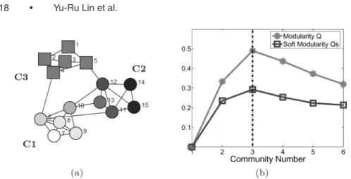
Fig. 5. The first synthetic dataset: (a) the static network, (b) modularity and soft modularity under different community numbers.
dataset was first studied in White and Smyth [2005] and is shown in Figure(5a). The network contains 15 nodes which roughly form 3 communities—C1, C2, andC3—where edges tend to occur between nodes in the same community. We first check our soft modularity measure. We apply our algorithm to the network with various community numbersm and the resulting Qsvalues are plotted in Figure(5b). In addition, in Figure(5b) we also show the modularity valuesQ that are reported in [White and Smyth 2005]. As can be seen from the plot, both Qsand Q show distinct peaks whenm =3, which corresponds to the correct community number.
Next, after our algorithm correctly partitions the 15 nodes into three munities, we illustrate the soft community membership by studying two com-munities among the three—C1 = {6, 7, 8, 9, 10}andC2 = {11, 12, 13, 14, 15}. In Figure(5a), we use the same circle shape to represent these 10 nodes but use different gray levels to indicate their community membership—we use white color to illustrate the level that a node belongs to C1 and dark color to show the level that a node belongs toC2. As can be seen, while node 7, node 14, and node 15 have very clear community memberships, node 10 and node 13, who are on the boundary betweenC1 andC2, have rather fuzzy membership. That is, our algorithm is capable of assigning meaningful soft membership to a node to indicate to which level the node belongs to a certain community.
6.1.2 Synthetic Dataset #2. The second dataset is generated according to the description in Newman and Girvan [2004]. This dataset contains 128 nodes, which are divided into 4 communities of 32 nodes each. We generate data for 50 consecutive timesteps. In each timestep from 2 to 50, dynamics are introduced in the following way: from each community we randomly select certain number of members to leave their original community and to join randomly the other three communities. Edges are added randomly with a higher probabilitypinfor within-community edges and a lower probability pout for between-community edges. However, the average degree for the nodes is set to 20. As a result, a single parameter z, which represents the mean number of edges from a node to nodes in other communities, is enough to describe the data. In this study, we
investigate two values forz:z=5 (which results inpin=0.05 and pout =0.16) where the community structure is clearer, andz =6 (which results inpin=0.06 and pout = 0.12) where the community structure is fuzzier. Furthermore, for each fixedz, we investigate two cases: the case where the community structure is relatively stable over time (with 10% members change their communities at each timestep) and the case where the community structures change more dramatically over time (with 30% members change their communities at each timestep).
We compare ourFacetNetframework with 3 baseline algorithms. The first baseline, which we callEvolSpec, is the evolutionary spectral clustering algo-rithm proposed in Chi et al. [2007]. BecauseEvolSpecis an evolutionary ver-sion of the Normalized Cut (NCut) algorithm in Shi and Malik [2000], we take NCutas our second baseline. Similarly,FacetNetis an evolutionary version of the soft clustering method (SNMF) in Yu et al. [2005], we takeSNMFas our third baseline. Notice thatFacetNetandEvolSpecare evolutionary algorithms whereasNCut andSNMFare not—NCut andSNMFwork on each snapshot graph independently of other snapshot graphs. In addition, to make the results comparable, forFacetNetandSNMFwe convert the soft membership into 0/1 indicators by assigning each node to the community it most likely belongs to. Furthermore, in all the experiments, forFacetNetandEvolSpecwe setαto be 0.8 (i.e.,ν=1/5).
For the performance metric, because we have the ground truth for the community memberships at each timestep, we directly study the error rate of the community structures obtained by different algorithms. The error rate is computed in the following way. The community structure computed by a given algorithm can be represented by a 128-by-4 indicator matrixZ, where thei-th row ofZ indicates the community membership of thei-th node (i.e., if thei-th node belongs to thek-th community, thenzik =1 andzik = 0 fork =k). A
similar indicator matrixG can be built for the ground truth. Then the error rate is represented by the norm Z ZT−GGT
F, which measures the distance between the community structure represented by Z and that represented by G(see Bach and Jordan [2006] for a detailed discussion). All the experiments are repeated 50 times with different random seeds and the average results are reported.
Figure 6 gives the performance on the two datasets withz=5. Figure 6(a) shows the adjacency matrix of the snapshot graph at the first timestep, where the nodes are ordered according to their truth community memberships so that the true community structure can be seen. As can be seen from the figure, the community structure is relatively easy to detect whenz =5. Figure 6(b) and Figure 6(c) show the error rates over time for the four algorithms for the cases of 10% and 30% nodes changing their communities at each timestep, respectively. From the figures we have the following observations. First, on these datasets, among the two nonevolutionary algorithms (NCut andSNMF), NCut outper-formsSNMF. Second, our algorithmFacetNetclearly outperforms the evolu-tionary spectral clustering algorithmEvolSpecin both cases. Third, when the community structure changes more dramatically over time, the benefit of the evolutionary spectral clustering disappears (in Figure 6(c),NCutandEvolSpec
Fig. 6. Error with respect to the ground truth over 50 timesteps on the datasets withz=5: (a) the adjacency matrix of the first timestep, (b) 10% nodes change their community at each timestep, (c) 30% nodes change their community at each timestep.
Fig. 7. Error with respect to the ground truth over 50 timesteps on the datasets withz=6: (a) the adjacency matrix of the first timestep, (b) 10% nodes change their community at each timestep, (c) 30% nodes change their community at each timestep.
have almost identical error rates) while the benefit of ourFacetNetalgorithm is still clearly visible.
Figure 7 gives the performance on the two datasets withz =6. Figure 7(a) shows the adjacency matrix of the snapshot graph at the first timestep, from which we can see that the community structure is more difficult to detect. Figure 7(b) and Figure 7(c) show the error rates over time for the four algo-rithms for the cases of 10% and 30% nodes changing their communities at each timestep, respectively. From the results we can see that on these two datasets,FacetNetstill outperforms other baseline algorithms although when the community structure changes dramatically (as shown in Figure 7(c)), the improvement ofFacetNetbecomes rather marginal.
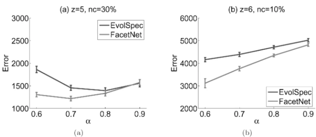
We study the performance over different values of α. Figure 8 reports the mean error rates (averaging over timesteps 2-50) of two evolutionary algorithms, EvolSpec and FacetNet, with error bars represent one standard
Fig. 8. Mean error rates (averaging over timesteps 2-50) of two evolutionary algorithms, with error bars represent one standard deviation: (a) on datasets withz=5, 30% nodes change their community every timestep, (b) on datasets withz=6, 10% nodes change their community every timestep.
deviation. Figure 8(a) and (b) show results on the same datasets as in Figure 6(c) and Figure 7(b). As can be seen, first, when decreasingα(i.e., em-phasize more on temporal smoothness), the improvement ofFacetNetagainst EvolSpecbecome more significant. Second, as shown in Figure 8(a), the mean error rates do not necessarily decrease with more temporal smoothness, i.e. smaller value ofα. This is expected because the importance of new observations are neglected. The results also suggestFacetNet can better tradeoff between new observation and temporal smoothness.
6.1.3 Synthetic Dataset # 3. Next, we study the time performance of FacetNet. We repeat the previous experiment over a family of networks of vari-ous sizes (node numbers). In Figure 9(a) we show the average running time per iteration of our algorithm on networks with different sizes (the algorithm is im-plemented in Matlab). In Figure 9(b) we showed the number of iteration needed for convergence when the convergence criterion is that the relative change in log likelihood between two consecutive iterations is below a threshold of 1e-5. As can be seen, first, the running time per iteration scales linearly with the size of network, which validates our theoretical analysis in Section 4.2; second, the number of iteration needed for convergence is insensitive to the network size, which implies that the overall running time of our algorithm scales linearly to the size of network.
6.2 NEC Blog Dataset
The blog data was collected by an NEC in-house blog crawler. Given seeds of manually picked highly ranked blogs, the crawler discovered blogs that are densely connected with the seeds, resulting in an expanded set of blogs that communicate with each other. The crawler then continued monitoring for new entries over a long time period. This NEC blog data set contains 148,681 entry-to-entry links among 407 blogs crawled during 12 consecutive month (a timestep
Fig. 9. Running time for networks of different sizes: (a) running time (sec) per each iteration), (b) number of iterations until converge.
Fig. 10. (a) Soft modularity and (b) mutual information under differentαfor the NEC Blog dataset.
is one month), between August 2005 and September 2006. Following [Ning et al. 2007], we defineW bywij=wij˜ /p,qwpq˜ where ˜wii=1, ˜wij=exp(−1/(γ ·lij)) ifeij∈Et, and otherwise ˜wij=0. In the formula,lijis the edge weight (e.g., # of links) ofeijandγ, which is set to 0.2, is a parameter to control marginal effect whenlijis increased.
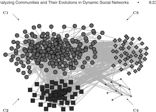
We start with analyzing the overall picture of the dataset. We first aggregate all the edges over all timesteps into a single network and apply our algorithm to compute the soft modularity scoreQsunder different community numbers. As can be seen in Figure 10(a), a clear peak shows when the community number is 4. We draw the aggregated graph in Figure 11, according to the main community each blog most likely belongs to. In addition, in Table I we list the top keywords, measured by thetf-idfscore, that occur in the entries of these four communities. It seems that C1 focuses on technology, C2 on politics, C3 on international entertainment, andC4 on digital libraries.
Next, we analyze the blog data as a dynamic network. After studying the content of the blogs, we find that the above four communities stay rather stable over all the timesteps. This effect is partially due to the way these blogs are selected by our focused crawler—our crawler chose to crawl a densely connected subgraph of the blogosphere where each node in the subgraph has large number of links and high level of interaction intensities. Therefore, most of the selected blogs belong to some well-known bloggers and they seldom move around be-tween communities. We apply ourFacetNetalgorithm on the data with different
Fig. 11. Four communities in the NEC Blog dataset.
Table I. Top Keywords Among the Four Communities in the NEC Blog Dataset, Sorted by the
tf-idfScore
C1 adsense, beta, skype, firefox, msn, rss, aol, yahoo, google, ebay, desktop, wordpress, voip, feeds, myspace, podcasting, technorati, search, engine, browser, ads, gmail, windows, os, developer, venture, marketing, apple, podcasts, developers, engines, mac, publishers, ceo, linux
C2 gop, uranium, hezbollah, democrats, rove, cia, republicans, saddam, qaeda, tax, republican, iraqi, roberts, bush, clinton, iraq, senate, troops, terrorists, administration, terrorist, wilson, conservative, taxes, liberal, intelligence, israel, terror, iran, weapons, war, soldiers
C3 shanghai, robots, installation, japan, japanese, architecture, art, chinese, china, saudi, phones, filed, mobile, games, korea, rfid, sex, green, camera, sound, cell, body, africa, phone, entertainment, film, gay, india, fuel, archive, design, elections, flash, device, water, wireless, south
C4 library, learning, digital, resources, collection, conference, staff, communities, students, session, books, database, access, survey, university, science, canada, myspace, articles, education, technologies, knowledge, filed, virtual, tools, research, david, learn, services, flickr, computers
α. Because there is no ground truth in this dataset, we instead use the commu-nities obtained from the aggregated graph (Figure 11) as a reference, and we compute the mutual information between the extracted communities at each timestep and the four communities shown in Figure 11. We refer interested readers to Xu et al. [2003] for detailed definition of the mutual information between two partitions. Basically, high mutual information between two parti-tions indicates that the two partiparti-tions are similar to each other.
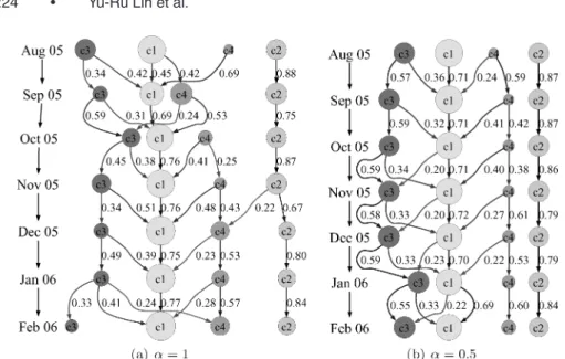
Fig. 12. The Evolution Net of the NEC Blog dataset when (a)α=1 and (b)α=0.5.
Figure 10(b) shows the mutual information results underα=0.1, 0.5, and 0.9. As can be seen, asαincreases, our algorithm emphasizes less on the tempo-ral smoothness and as a result, the community structure has higher variation over time. In addition, asαincreases, the communities at each timestep deviate further from the communities obtained from the aggregated data. These results on one hand justify our arguments in the introduction section and on the other hand demonstrate that our FacetNetframework is capable of controlling the tradeoff between the snapshot cost and the temporal cost in the cost function Equation (3).
Figure 12 shows the Evolution Net derived from our framework whenα=1 and 0.5 (α=1 means no temporal smoothness is considered). In the Evolution Net, the size of a node is proportional toλkand it represents the size of the cor-responding community. The edge label indicates the probability of a transition from the source community att-1to the target community att. (To avoid clutter, we did not show edges with probabilities less than 0.2). From Figure 12(a) we see that when no temporal smoothness is considered,C4 disappeared at the second timestep (Sep 2005) and reappeared in the third timestep (Oct 2005). However, by carefully examining the original data, we did not find any significant events so support such changes. Therefore, we conjecture that these changes are due to the data noises at the second timestep, which triggered the algorithm to split C1 into two communities and mergeC4 to one of them. In comparison, as can be seen from Figure 12(b), when there is a temporal smoothness term, the four communities remain relatively stable. That is, although there exist transitions among different types of communities, the majority of transitions are between communities of the same type. These results demonstrate that the FacetNet framework is more robust to data noise.
From the Evolution Net, we can also obtain some other observations. For ex-ample, the political communityC2 is rather isolated from the rest communities
Fig. 13. The Community Net for the NEC Blog dataset in September 2005.
over all the time. In comparison, bothC3 andC4 interacts withC1 heavily. In addition, in Figure 13 we show the Community Net at an arbitrary timestep (Sep 2005). In the Community Net, the node sizes are proportional toλt;kand the edge weights are proportional to the corresponding entries intXTt Dt−1Xtt (self-loops are not shown). We can see that this Community Net is a good syn-opsis of the aggregated network in Figure 11.
6.3 DBLP Coauthorship Dataset
The DBLP coauthorship dataset is described in Asur et al. [2007]. It con-tains the coauthorship information among the papers in 28 conferences over 10 years (1997–2006). The 28 conferences span three main areas—data mining, database, and artificial intelligence. By removing authors with too few papers or too few coauthors in the dataset, we select 1,071 authors from the original dataset and build snapshot graphs with these 1,071 authors as nodes. The ag-gregated coauthorship graph among these authors is given in Figure 14. For analyzing community evolutions, we aggregate data in every two years into one timestep and therefore we have 5 timesteps in total (and therefore 5 snapshot graphs) for the dynamic network. In the experiments, we fixed the community numberm to be 3, which corresponds to the number of main research areas among the 28 conferences.
In the first experiment, we apply theFacetNetalgorithm on the aggregated coauthorship graph and in Table II we list the extracted top authors in the 3 communities, where the rank is determined by the valuexik, that is, pk→i. Recall that pk→i indicates to what level thek-th community involves thei-th node. So from our framework, we can directly infer who are the important mem-bers in each community. However, notice that byimportant, we are not judging the quality or quantity of papers by an author. Instead, in our framework the importance of a node in a community is determined by its contribution to the community structure.
In the second experiment, we apply ourFacetNetalgorithm on the snapshot graphs over 5 timesteps (withα=0.9 or equivalentlyν =1/9). Using the so-lution of our algorithm, we examine some individual authors listed in Table II and see how their community membership change over time. It turns out that
Fig. 14. The aggregated coauthorship graph among the 1,071 authors in the DBLP dataset.
the top authors in the Artificial Intelligence community remain very focused over all timesteps—most of them have xik =0 when kdoes not correspond to the AI community. In contrast, a couple of authors in the Data Mining (DM) community and the Database (DB) community switched their community mem-bership during the 10 year period covered by the dataset. For one example, in Figure 15 we demonstrate one top author (Philip S. Yu) in the DM commu-nity whose commucommu-nity membership remains stable over all the timesteps and another top author (Laks V. S. Lakshmanan) whose community membership varies very much over the 5 timesteps. In the figure, each compass indicates a pair (pk1→i,pk2→i) wherek1andk2correspond to the DB and the DM
communi-ties, respectively. So in a compass, a vertical arrow (which has a large projection on the y-axis) indicates a large value of the community membership in the DM community and a horizontal arrow (which has a large projection on thex-axis) indicates a large value of the community membership in the DB community. From Figure 15 we can see that the first author consistently played an im-portant role mainly in the DM community, whereas the second author had a varying role in both the two communities. By looking at the publication record of this second author we can see that he had published on the topic of asso-ciation rules (DM) during the periods of t = 1997–1998 and t = 2001–2002. However, during the periods of t=1999–2000 andt=2003–2006, this author co-authored a large number of papers in top DB conferences (e.g., 15 papers in SIGMOD and 12 in VLDB), which is reflected by his high values of membership in the DB community (large projections on thex-axis) during these periods.