WORKING PAPER
2007-07
Resource
Economics
and Policy Analysis
(REPA)
Research Group
Department of Economics
University of Victoria
Bayesian Model Averaging in the Context of Spatial
Hedonic Pricing: An Application to Farmland Values
Geerte Cotteleer, Tracy Stobbe,
and G. Cornelis van Kooten
ii
REPA Working Papers:
2003-01 – Compensation for Wildlife Damage: Habitat Conversion, Species Preservation and Local Welfare (Rondeau and Bulte)
2003-02 – Demand for Wildlife Hunting in British Columbia (Sun, van Kooten and Voss) 2003-03 – Does Inclusion of Landowners’ Non-Market Values Lower Costs of Creating Carbon
Forest Sinks? (Shaikh, Suchánek, Sun and van Kooten)
2003-04 – Smoke and Mirrors: The Kyoto Protocol and Beyond (van Kooten)
2003-05 – Creating Carbon Offsets in Agriculture through No-Till Cultivation: A Meta-Analysis of Costs and Carbon Benefits (Manley, van Kooten, Moeltne, and Johnson)
2003-06 – Climate Change and Forest Ecosystem Sinks: Economic Analysis (van Kooten and Eagle)
2003-07 – Resolving Range Conflict in Nevada? The Potential for Compensation via Monetary Payouts and Grazing Alternatives (Hobby and van Kooten) 2003-08 – Social Dilemmas and Public Range Management: Results from the Nevada
Ranch Survey (van Kooten, Thomsen, Hobby and Eagle)
2004-01 – How Costly are Carbon Offsets? A Meta-Analysis of Forest Carbon Sinks (van Kooten, Eagle, Manley and Smolak)
2004-02 – Managing Forests for Multiple Tradeoffs: Compromising on Timber, Carbon and Biodiversity Objectives (Krcmar, van Kooten and Vertinsky)
2004-03 – Tests of the EKC Hypothesis using CO2 Panel Data (Shi)
2004-04 – Are Log Markets Competitive? Empirical Evidence and Implications for Canada-U.S. Trade in Softwood Lumber (Niquidet and van Kooten)
2004-05 – Conservation Payments under Risk: A Stochastic Dominance Approach (Benítez, Kuosmanen, Olschewski and van Kooten)
2004-06 – Modeling Alternative Zoning Strategies in Forest Management (Krcmar, Vertinsky and van Kooten)
2004-07 – Another Look at the Income Elasticity of Non-Point Source Air Pollutants: A Semiparametric Approach (Roy and van Kooten)
2004-08 – Anthropogenic and Natural Determinants of the Population of a Sensitive Species: Sage Grouse in Nevada (van Kooten, Eagle and Eiswerth)
2004-09 – Demand for Wildlife Hunting in British Columbia (Sun, van Kooten and Voss)
2004-10 – Viability of Carbon Offset Generating Projects in Boreal Ontario (Biggs and Laaksonen- Craig)
2004-11 – Economics of Forest and Agricultural Carbon Sinks (van Kooten)
2004-12 – Economic Dynamics of Tree Planting for Carbon Uptake on Marginal Agricultural Lands (van Kooten) (Copy of paper published in the Canadian Journal of Agricultural Economics 48(March): 51-65.)
2004-13 – Decoupling Farm Payments: Experience in the US, Canada, and Europe (Ogg and van Kooten)
2004–14 – Afforestation Generated Kyoto Compliant Carbon Offsets: A Case Study in Northeastern Ontario (Biggs)
2005–01 – Utility-scale Wind Power: Impacts of Increased Penetration (Pitt, van Kooten, Love and Djilali)
2005–02 – Integrating Wind Power in Electricity Grids: An Economic Analysis (Liu, van Kooten and Pitt)
iii
Lumber (Biggs, Laaksonen-Craig, Niquidet and van Kooten)
2005–04 – Can Forest Management Strategies Sustain The Development Needs Of The Little Red River Cree First Nation? (Krcmar, Nelson, van Kooten, Vertinsky and Webb)
2005–05 – Economics of Forest and Agricultural Carbon Sinks (van Kooten)
2005–06 – Divergence Between WTA & WTP Revisited: Livestock Grazing on Public Range (Sun, van Kooten and Voss)
2005–07 – Dynamic Programming and Learning Models for Management of a Nonnative Species (Eiswerth, van Kooten, Lines and Eagle)
2005–08 – Canada-US Softwood Lumber Trade Revisited: Examining the Role of Substitution Bias in the Context of a Spatial Price Equilibrium Framework (Mogus, Stennes and van Kooten)
2005–09 – Are Agricultural Values a Reliable Guide in Determining Landowners’ Decisions to Create Carbon Forest Sinks?* (Shaikh, Sun and van Kooten) *Updated version of Working Paper 2003-03
2005–10 – Carbon Sinks and Reservoirs: The Value of Permanence and Role of Discounting (Benitez and van Kooten)
2005–11 – Fuzzy Logic and Preference Uncertainty in Non-Market Valuation (Sun and van Kooten) 2005–12 – Forest Management Zone Design with a Tabu Search Algorithm (Krcmar, Mitrovic- Minic, van Kooten and Vertinsky)
2005–13 – Resolving Range Conflict in Nevada? Buyouts and Other Compensation Alternatives (van Kooten, Thomsen and Hobby) *Updated version of Working Paper 2003-07
2005–14 – Conservation Payments Under Risk: A Stochastic Dominance Approach (Benítez, Kuosmanen, Olschewski and van Kooten) *Updated version of Working Paper 2004-05 2005–15 – The Effect of Uncertainty on Contingent Valuation Estimates: A Comparison (Shaikh,
Sun and van Kooten)
2005–16 – Land Degradation in Ethiopia: What do Stoves Have to do with it? (Gebreegziabher, van Kooten and.van Soest)
2005–17 –The Optimal Length of an Agricultural Carbon Contract (Gulati and Vercammen) 2006–01 – Economic Impacts of Yellow Starthistle on California (Eagle, Eiswerth, Johnson,
Schoenig and van Kooten)
2006–02 – The Economics of Wind Power with Energy Storage (Benitez, Dragulescu and van Kooten)
2006–03 – A Dynamic Bioeconomic Model of Ivory Trade: Details and Extended Results (van Kooten)
2006–04 –The Potential for Wind Energy Meeting Electricity Needs on Vancouver Island (Prescott, van Kooten and Zhu)
2006–05 – Network Constrained Wind Integration: An Optimal Cost Approach (Maddaloni, Rowe and van Kooten)
2006–06 – Deforestation (Folmer and van Kooten)
2007–01 – Linking Forests and Economic Well-being: A Four-Quadrant Approach (Wang, DesRoches, Sun, Stennes, Wilson and van Kooten)
2007–02 – Economics of Forest Ecosystem Forest Sinks: A Review (van Kooten and Sohngen)
2007–03 – Costs of Creating Carbon Offset Credits via Forestry Activities: A Meta-Regression Analysis (van Kooten, Laaksonen-Craig and Wang)
2007–04 – The Economics of Wind Power: Destabilizing an Electricity Grid with Renewable Power (Prescott and van Kooten)
2007–06 –Farmland Conservation in The Netherlands and British Columbia, Canada: A Comparative Analysis Using GIS-based Hedonic Pricing Models (Cotteleer, Stobbe and van Kooten) 2007–07 –Bayesian Model Averaging in the Context of Spatial Hedonic Pricing: An Application to
Farmland Values (Cotteleer, Stobbe and van Kooten)
For copies of this or other REPA working papers contact: REPA Research Group
Department of Economics
University of Victoria PO Box 1700 STN CSC Victoria, BC V8W 2Y2 CANADA Ph: 250.472.4415
Fax: 250.721.6214
www.vkooten.net/repa
This working paper is made available by the Resource Economics and Policy Analysis (REPA) Research Group at the University of Victoria. REPA working papers have not been peer reviewed and contain preliminary research findings. They shall not be cited without the expressed written consent of the author(s).
Partial funding for this project was provided by the Farm Level Policy Agricultural Policy Research Network (APRN). The APRN is funded by Agriculture and Agrifood Canada.
Bayesian Model Averaging in the Context of Spatial Hedonic Pricing:
An Application to Farmland Values
by
Geerte Cotteleer1, Tracy Stobbe2, and G Cornelis van Kooten2
1 Agricultural Economics and Rural Policy, Department of Social Sciences,
Wageningen University, Wageningen, The Netherlands
2 Department of Economics, University of Victoria, Victoria, B.C., Canada
Date: December 18, 2007
Abstract
Since 1973, British Columbia created an Agricultural Land Reserve to protect farmland from development. In this study, we employ GIS-based hedonic pricing models of farmland values to examine factors that affect farmland prices. We take spatial lag and error dependence into explicit account. However, the use of spatial econometric techniques in hedonic pricing models is problematic because there is uncertainty with respect to the choice of the explanatory variables and the spatial weighting matrix. Bayesian model averaging techniques in combination with Markov Chain Monte Carlo Model Composition are used to allow for both types of model uncertainty.
Key Words: Bayesian model averaging, Markov Chain Monte Carlo Model Composition, spatial econometrics, hedonic pricing, GIS, urban-rural fringe, farmland fragmentation
JEL Categories: R11, R15, C50, R14.
Copyright 2007 by Geerte Cotteleer, Tracy Stobbe and G. Cornelis van Kooten. All rights reserved. Readers may make verbatim copies of this document for non-commercial purposes by any means, provided that this copyright notice appears on all such copies.
Bayesian Model Averaging in the Context of Spatial Hedonic Pricing:
An Application to Farmland Values
1. Introduction
As cities grow and spread into the countryside, agricultural land is often the first victim of urban development. Despite programs and laws to protect agriculture, farmland prices in the rural-urban interface have increased significantly, often beyond the reach of farmers wishing to enter the sector or expand their operations. Because land prices are driven by the development and not agricultural potential of land, farming near urban areas becomes more difficult both financially and logistically. As more and more land is developed into residential subdivisions and transport corridors, remaining farmland becomes increasingly fragmented. Farmers often need to buy or lease fields that are not contiguous, so they are unable to combine fields of
sufficiently large size to take advantage of scale economies. Farmers incur higher transportation costs for moving equipment, animals and produce; encounter more nuisance complaints concerning odors, noise and slow-moving farm vehicles; and experience higher rates of trespass and vandalism.
In the current study, we examine the effect of urban encroachment on farming near Victoria, the capital of British Columbia, Canada’s westernmost province. BC’s agricultural land is limited, with the most productive land located near the most-rapidly growing urban centers – Vancouver, Victoria and Kelowna in the Okanagan Valley in the Interior. To protect the 1.1% of the Province considered prime farmland from development, the government created the Agricultural Land Reserve (ALR) in 1973. The ALR is a zoning ordinance that prevents agricultural land from being subdivided or used for non-agricultural purposes without permission from the Agricultural Land Commission (ALC). The ALR permits only one dwelling per
parcel, which is intended to serve as a farmer’s residence.
Speculation by developers and purchases of farmland for residential purposes (rural estates) are the main factors that drive up agricultural land prices near urban centers. We seek to determine empirically whether speculation in anticipation of changing land designation is happening on ALR land. We hypothesize that, if zoning is credible, farmland prices adjacent to the urban edges should be lower due to the reduced productivity associated with negative urban externalities (Nelson, 1992). Alternatively, if landowners do not believe agricultural protection is permanent, these lands will have higher values in expectation that it will be sold to developers in the future.
We employ a GIS-based hedonic pricing model to quantify ALR specific measures and investigate characteristics that contribute to farmland prices near the urban fringe. We also employ spatial econometric techniques that take into account spatial dependencies that are not incorporated as covariates in the hedonic pricing model. The problem with spatial econometric techniques is that they require a priori specification of a weighting matrix of spatial relations between observations, although choice of a specific relationship is arbitrary (Anselin, 1988). Another problem is that there is little in the way of theory to guide the choice of the covariates to be included in the hedonic pricing model. This means that there is both parameter uncertainty and uncertainty in the choice of the spatial weighting matrix.
Our objective is, therefore, to investigate whether the ALR has been effective in preserving farmland near Victoria, but in a way that resolves uncertainty in the application of the spatial hedonic pricing model. To address the latter issue, we apply Bayesian Model Averaging in combination with Markov Chain Monte Carlo Model Composition (MC3) to deal with model uncertainty. The benefit of Bayesian Model
Averaging is that it does not assume there is only one correct model specification; rather, final parameter estimates are weighted averages based on a whole range of possible model specifications, including different explanatory variables and different specifications of the weighting matrix. Furthermore, the MC3 framework makes sure that model specifications with high posterior probabilities are taken into account in the weighted averages.
Although the MC3 framework has been extended to spatial econometric models by LeSage and Parent (2007), and LeSage and Fischer (2007), the current research explicitly incorporates the selection of different specifications of the
weighting matrix (based on nearest neighbors, distances and spatiotemporal patterns) in both MC3 procedures for the spatial lag and error dependence models. To our knowledge, this extension of the MC3 procedure constitutes an additional contribution of our research.
The outline of the paper is as follows. Section 2 introduces the framework for the spatial hedonic pricing model with Bayesian model averaged results. This section also discusses the MC3 procedure. The data and variables constructed for the hedonic
pricing model are discussed in section 3, as is our study area. In section 5 the empirical results are presented and discussed. Section 6 concludes.
2. A Bayesian Approach to Hedonic Pricing Model Specification
To investigate the impact of BC’s Agricultural Land Reserve (ALR) and such things as land fragmentation on farmland prices, we specify a hedonic pricing model as follows (Rosen, 1974):
(1) P = αι+ Xβ + ε,
vector of associated coefficients to be estimated, αis a constant to be estimated and ι an associated vector of ones,and ε is a vector of error terms.
Spatial lag or error dependence
Given the spatial nature of the data, it is important to incorporate spatial dependence in the model. Spatial dependence can be incorporated as spatial lag or spatial error dependence. A general formulation that includes both is (Anselin, 1988):
(2) P = αι+ ρW1P + Xβ + u, with u = λW2u + ε and ε ~ N(0, σ2I),
where W1and W2are spatial weighting matrices. The spatial weights are specified a priori between all pairs of observations. In our model, where each observation i
corresponds to a farmland sales transaction, each element wij weights the degree of spatial dependence according to the proximity or distance between parcel i and any other parcel j; ρis the coefficient of the spatial lag dependence structure; and λ is the coefficient in a spatial autoregressive structure for the error term.
Equation (2) represents the classic linear regression model if ρ=0 and λ=0. When λ=0 and ρ≠0, (2) represents the Spatial Autoregressive (SAR) model, which takes spatial lag dependence explicitly into account. This form of spatial dependence may exist when sellers and buyers use prices of parcels that were recently sold in the neighborhood as a reference point. If ρ=0 and λ≠0, we have the Spatial Error Model (SEM) that takes spatial error dependence into account. Spatial error dependence (or spatial autocorrelation) arises if there is spatial interaction between the residuals due to unobserved or omitted variables that have spatial patterns.
The choice of the spatial weighting matrix
Lacking guidance regarding the choice of a weighting matrix, we specify a variety of different types: Several variations employ binary weights, two are based on
distances, and two are based on spatiotemporal patterns. In the case of binary weights, an element in the weighting matrix equals one if two observations are considered to be neighbors and zero if not. The first binary weighting matrix is based on Delaunay triangulation (Zhang and Murayama, 2000), which uses non-overlapping triangles with the centroids of parcels as the vertices of the triangles. For each parcel, first-order neighbors are defined as those parcels that are directly connected to it by the edges of a triangle. Other variants of the binary weighting approach employ n-order neighbors, defined as the n neighbors that are closest in distance terms. In a weighting matrix based on n-order neighbors, there are n entries equal to one in each row. Thus, if one considers the three nearest neighbors then each row in the weighting matrix will have three elements equal to one (with zeros on the diagonal). We consider as many as ten possible neighbors. As Bucholtz (2004) points out, matrices based on a specific number of nearest neighbors have an advantage over other weighting matrices
because the hypothesized spatial influence that parcels have on each other is not changed if the matrix is row-standardized (so that the sum of elements in each row equal one). Row-standardization is used for computational purposes. The number of nearest neighbors in the Delaunay-based weighting matrix depends on the number of edges within the triangulation that connect vertices. Thus, each row may have a varying number of elements equal to 1. Both matrices based on nearest neighbors and the Delaunay-triangulation are sparse, with many zeros and few ones. Sparse matrix calculations require much less computer memory and storage space (LeSage, 1998).
For weighting matrices based on distances, one employs inverse distances (1/d) and the other inverse squared distances (1/d2). Thus, the weights are greatest for the nearest parcels. For inverse squared distances, the weights decline at an increasing rate as parcels are farther apart. The advantage of the inverse distance-based matrices
is that they take the relationship between all parcels into account, but a disadvantage is that the weighting matrices are full, with only zero elements on the diagonal, making computation more difficult.
For the spatiotemporal weighting matrices, observations are ordered so that the resulting spatial weighting matrix is lower-triangular. Elements are based on the inverse distance and the inverse squared distances between parcels. The advantage in this case is that spatiotemporal weighting assumes sale prices are influenced by the sales of neighboring properties, but (of course) only if the neighboring properties were sold earlier in time (Pace, et al., 1998).
Bayesian model averaging and the MC3 procedure
Because there is uncertainty about which weighting matrix and set of explanatory variables to use in our hedonic pricing model, we employ Bayesian techniques that allow us to specify posterior model probabilities for each specific model we wish to consider. These model probabilities tell us how likely it is that a given model is the correct one. Rather than basing parameter estimates only on the model with the highest posterior probability, we use Bayesian Model Averaging and weight the estimates of the whole range of potential models with the posterior model probabilities, which are given by (Koop, 2003):
(3)
∑
= = M m m m i i i M p M y p M p M y p y M p 1 ) ( ) | ( ) ( ) | ( ) | (where p(y|Mi) is the marginal likelihood that model Mi is the correct one and p(Mi) are the prior model probabilities. If, a priori, the researcher considers each model to be equally likely, all prior model probabilities are equal to 1/M, where M is the total number of models to be considered. In this case the posterior model probabilities are
determined only by the marginal likelihoods. The marginal likelihood for model i is (Koop, 2003):
(4) p(y|Mi)=
∫
p(y|θ,Mi)p(θ |Mi)dθ,where p(y|θ,Mi) is the likelihood and p(θ|Mi) is the prior for the parameter vector θ. In our case, θ includes either [α, β, σ2, λ] or [α, β, σ2, ρ], depending on whether one considers the spatial error or lag model. The specifications of the marginal likelihoods for the spatial lag and error dependence models are provided in LeSage and Parent (2007). Their specifications are based on prior information on α, β and σ2 from Fernandez, Ley and Steel (2001), and they assume a beta-prior centered about ρ=0 and λ=0. Given that we have no information on these parameters, we assume the same priors despite their uninformative nature; however, as illustrated below, with Bayesian updating, we eventually rely on the data rather than the priors.
To derive the posterior model probabilities, we need to consider each possible model specification. With k potential explanatory variables and δ potential
specifications of the weighting matrix, there are 2k×δ models to consider, which is practically infeasible. (For example, with k=21 and δ=6, there are 12,582,912 models to consider.) Therefore, we use Markov Chain Monte Carlo Model Composition (Madigan, et al., 1995). The stochastic process generated by MC3 explores regions of the model space with high posterior model probabilities. The number of iterations in the MC3 procedure is pre-specified. At the start of the Markov chain, a regression model is chosen at random. Suppose the current model is Mi. The model that is proposed in the next step of the chain has either one variable more than the current model (‘birth step’), one variable less than Mi (‘death step’), or one variable of Mi replaced by a variable not currently in the model (‘move step’). The proposed model
by:
(5) p(accept new model) = ⎥ ⎦ ⎤ ⎢ ⎣ ⎡ ) | ( ) | ( , 1 min y M p y M p i j
A random draw using the probability from (5) of accepting the new model and not accepting it determines whether the new model indeed replaces the old, whether Mj replaces Mi.
This procedure for proposing new models is extended by LeSage and Fischer (2007) to include uncertainty with respect to the choice of the spatial weighting matrix in the MC3 procedure. However, only different numbers and types of nearest neighbor based weighting matrices are included in their procedure. As indicated above, we specify weighting matrices based on upwards of ten nearest neighbors, as well as ones based on Delaunay triangulation, distances and spatiotemporal patterns. However, we first use the method of LeSage and Fischer (2007) to sort out which of the nearest-neighbors’ weighting matrix to consider – one of the matrices with one to ten nearest neighbors; we select the binary weighting matrix with the number of nearest neighbors that had the highest model probability of being included. In addition, we extend this procedure by employing the MC3 procedure that considers six different weighting matrices (two binary, two distance based, and two
spatiotemporal).
We begin the MC3 procedure by considering a regression model with a randomly selected weighting matrix and randomly selected variables. Next we use 100,000 iterations to determine posterior model probabilities for each of the models visited during one of the 100,000 iterations. Each iteration involves the following steps:
Current model: Mi
Step 1: Toss a fair die with two sides 1s, two sides 2s and two sides 3s Outcome Decision
1. Exclude variable from model at random
2. Add at random a new explanatory variable not currently in model
3. Drop current explanatory variable at random from model; replace with randomly chosen explanatory variable not now in model
Choose new model Mj over Mi with probability given by (5). Step 2: Toss a coin
Outcome Decision
Heads Retain current weighting matrix (retain model Mj or Mi)
Tails Choose new weighting matrix at random from those not currently in model (Choose new model Mj+ over Mj or Mi with probability given by (5).
Model for next iteration: Mm = one of (Mj+, Mj, Mi) is chosen with some probability.
LeSage and Fischer (2007) point out that step 2 is valid as long as the probabilities of change versus no change in the weighting matrix are equal, which is true for a fair coin toss.
Inclusion probabilities for variables
Based on the MC3 procedure, for each variable we can calculate the
probabilities that this variable should be included in the model. Inclusion probabilities for variables are calculated as the number of times a variable is included in a model
that was accepted divided by the total number of iterations (draws). This differs from the inclusion probabilities in LeSage and Parent (2007). They base the inclusion probabilities on the number of times a variable is included in each unique proposed model. We argue that our measure better reflects the inclusion probabilities for two reasons: Although they might be unique, proposed models can be rejected and, therefore, they do not always have high posterior model probabilities. Further, we rather base our estimate on the total number of draws, instead of the number of unique proposed models.
3. Data and Variables
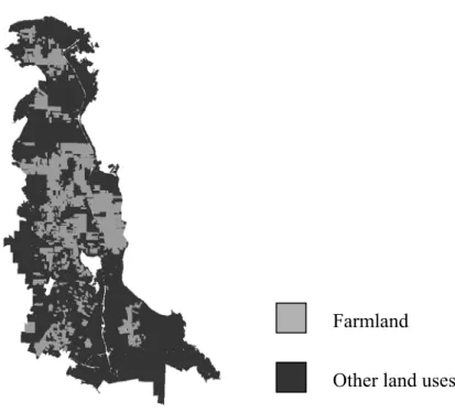
Our study area is the Saanich Peninsula of southern Vancouver Island, a rich agricultural area just north of Victoria (Figure 1). Together with the Fraser Valley and Okanagan, this area is home to the most important agricultural land in the Province, but it is also near one of the Province’s largest and rapidly growing urban centers. Hence, it experiences intense development pressure.
We use 533 observations of farmland parcels that were sold in the period 1974 (the year following creation of the ALR) to 2006. The data include all ‘single cash’ transactions but exclude sales that incorporated more than one parcel. A dummy variable (‘vacant land’) is used to distinguish between properties that do or do not have substantial structures, such as farmhouses, barns, poultry and milking facilities, etc. Only parcels were selected that could be linked to all fifteen datasets we used, so that for each observation all explanatory variables were available. Finally, if
properties were sold more than once, we included only the most recent transaction in our analysis, because the structure of our weighting matrices cannot handle multiple sales of the same property. In total, 3,688 farm sale transactions are available, of which 3,201 are from the period after 1973. Of these, 1,015 were single property cash
transactions, while the remaining 2,186 transactions were either multiple property cash transactions or non-cash transactions. The number of observations was further reduced to 932 as a result of linking issues between different datasets. Finally, it was reduced to 533 observations once earlier transactions of the same property were removed.
Farmland Other land uses
Source: Ministry of Agriculture and Lands and the Capital Regional District, edited map
Figure 1: Distribution of land use on the Saanich peninsula
The different data sets come from the B.C. Ministry of Agriculture and Lands, the B.C. Assessment Authority, other government agencies, and private sources. The GIS-based hedonic pricing model uses the per hectare market value of land as the dependent variable; the covariates include size of the farmland parcel, type of farm, topographical features of the land, a fragmentation index, distance to Victoria, an ALR dummy variable and the number of hectares excluded from the ALR each year.
place in 2005. However, this boundary has changed over the period 1974-2006, because exclusions of ALR land have taken place. To take this dynamic aspect of the ALR into account, we included the number of hectares that were excluded from the ALR as a covariate.
The fragmentation index is specified as the percentage of the perimeter bordering other farmland parcels multiplied by the size of the total farm block of all the farmland that is adjacent to the parcel. This index is designed to capture the importance of both the proximity to other farms and the total size of the farm block of which the parcel is a part.
Finally, we include macro variables, such as the mortgage rate and GDP, to account for the time span involved and because of their likely impact on farmland prices. We assume that, by including these macro-economic variables, time related fluctuations in farmland prices are sufficiently taken into account. We do not deflate property values, mainly because of lack of an appropriate deflator for property values for this region.
We specified a double-log functional form, where both the dependent and (where possible) the independent variables are in logarithmic form. This functional form is generally preferred over linear ones because linear functional forms have the disadvantage that they enable parcel characteristics easily to be repackaged,
precluding nonlinearities as a result of arbitrage (Rosen, 1974).
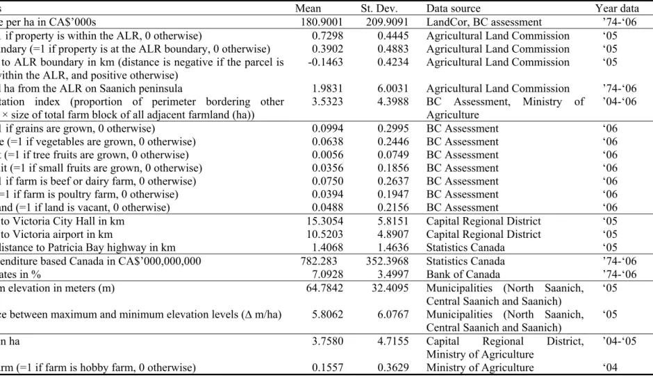
An overview of all the variables included in the hedonic pricing model as well as the data sources used to construct these variables are provided in Table 1.
Table 1: Summary statistics of variables included in hedonic pricing model (n = 533) and data sources
Variables Mean St. Dev. Data source Year data
Sale price per ha in CA$’000s 180.9001 209.9091 LandCor, BC assessment ’74-‘06
ALR (= 1 if property is within the ALR, 0 otherwise) 0.7298 0.4445 Agricultural Land Commission ‘05 ALR boundary (=1 if property is at the ALR boundary, 0 otherwise) 0.3902 0.4883 Agricultural Land Commission ‘05 Distance to ALR boundary in km (distance is negative if the parcel is
located within the ALR, and positive otherwise)
-0.1463 0.4234 Agricultural Land Commission ‘05
Excluded ha from the ALR on Saanich peninsula 1.9831 6.0031 Agricultural Land Commission ’74-‘06
Fragmentation index (proportion of perimeter bordering other farmland × size of total farm block of all adjacent farmland (ha))
3.5323 4.3988 BC Assessment, Ministry of
Agriculture
’04-‘06
Grain (=1 if grains are grown, 0 otherwise) 0.0994 0.2995 BC Assessment ‘06
Vegetable (=1 if vegetables are grown, 0 otherwise) 0.0638 0.2446 BC Assessment ‘06
Tree fruit (=1 if tree fruits are grown, 0 otherwise) 0.0056 0.0749 BC Assessment ‘06
Small fruit (=1 if small fruits are grown, 0 otherwise) 0.0356 0.1856 BC Assessment ‘06
Cows (=1 if farm is beef or dairy farm, 0 otherwise) 0.0750 0.2637 BC Assessment ‘06
Poultry (=1 if farm is poultry farm, 0 otherwise) 0.0394 0.1947 BC Assessment ‘06
Vacant land (=1 if land is vacant, 0 otherwise) 0.0488 0.2156 BC Assessment ‘06
Distance to Victoria City Hall in km 15.3054 5.8151 Capital Regional District ‘05
Distance to Victoria airport in km 10.5203 4.8907 Capital Regional District ‘05
Nearest distance to Patricia Bay highway in km 1.4068 1.4636 Statistics Canada ‘05
GDP expenditure based Canada in CA$’000,000,000 782.283 352.3968 Statistics Canada ’74-‘06
Interest rates in % 7.0928 3.4997 Bank of Canada ’74-‘06
Maximum elevation in meters (m) 64.7842 32.4095 Municipalities (North Saanich,
Central Saanich and Saanich)
‘05 Difference between maximum and minimum elevation levels (∆m/ha) 5.8062 6.0767 Municipalities (North Saanich,
Central Saanich and Saanich)
‘05
Lot size in ha 3.7580 4.7155 Capital Regional District,
Ministry of Agriculture
’04-‘05
Because the Saanich Peninsula is a well-defined area surrounded by ocean and fairly hilly, with only one city (Victoria) playing a significant role, there is a problem with multicollinearity – many of the covariates are inherently highly correlated. For example, the fragmentation measure is related to the ALR designation because farmland within the ALR is less fragmented than farmland outside the ALR.
Likewise, elevation is correlated with distance to the highway because the highlands are located in the western part of the Peninsula whereas the main north-south highway runs along the lower eastern section. Finally, distance to the Swartz Bay ferry
terminal on the northern tip of the Peninsula and distance to Victoria on the southern end are almost perfectly correlated. We address the multicollinearity problem by using Bayesian Modeling Averaging techniques. This means that each specific model includes different sets of variables, and therefore not all explanatory variables have to be included at once.
4. Empirical Results and Discussion
The Bayesian model averaged estimates are not based on all unique models visited in each of the 100,000 iterations. Means and t-statistics for the coefficients are only calculated for the 1000 models with the highest marginal likelihoods in the spatial lag specifications and the 200 ‘best’ models in the spatial error specifications. The reason that less models are used for the spatial error specifications is that it is simply too time consuming to calculate the means and dispersion measures for more than 200 models – the combination of 200 models and 5000draws per model took about 60 hours. For the spatial lag specifications, the combination of 1000 models and 10,000 draws per model takes about 10 hours. For the spatial lag specifications, 100,000 draws in the MC3 procedure produces18,164unique models. For the spatial error specifications we find 8,535 unique models in 100,000 draws.
With respect to the spatial error and lag structure, we conclude that both λ and ρ are significant and have a positive sign as expected. However, the t-statistic
(t=377.06) for the coefficient for spatial error dependence λ is much higher than the t-statistic for ρ (t=3.82). By directly comparing the marginal likelihoods of the best specifications of both SAR and SEM with the Bayes factor, we end up comparing SAR and SEM models with the explanatory variables lot size, GDP and vacant land, and the distance-based weighting matrix. The Bayes factor is often used to compare two model specifications assuming that prior model probabilities are the same. For the SEM versus SAR models, this factor is almost 1, indicating that the SEM model has a much higher marginal likelihood than the SAR model. Both the Bayes factor and the coefficients for spatial dependence indicate that SEM specifications are preferred over SAR specifications. Therefore, we only present the results for the SEM specification.
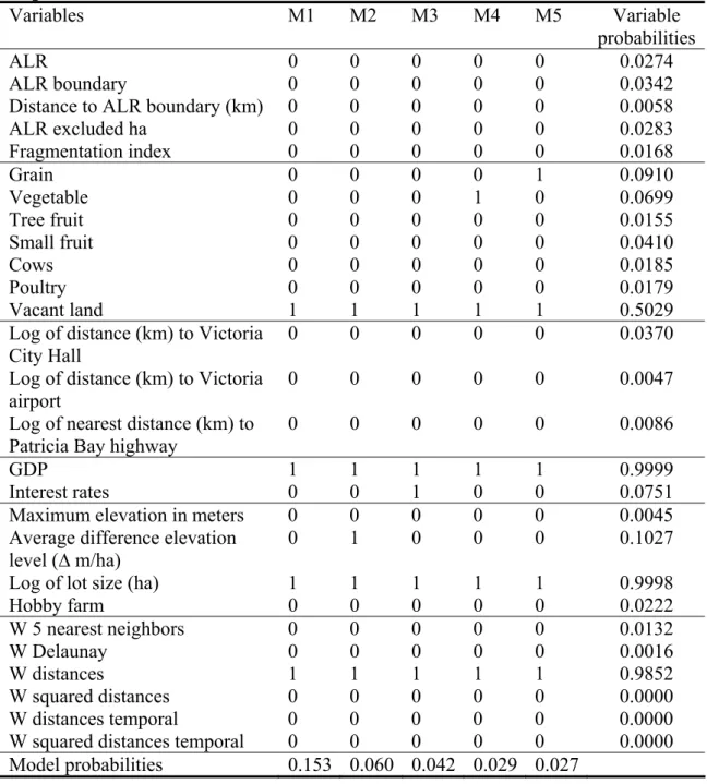
The specifications of the five models with the highest posterior model
probabilities resulting from the MC3 procedures are provided in Table 2. In this table, ones indicate the inclusion of a certain variable or weighting matrix and zeros indicate exclusion. Posterior model probabilities for the five ‘best’ models and probabilities for the inclusion of each of the variables and spatial weighting matrices are also presented in Table 2. The Bayesian model averaged means and t-statistics for β,σ2 andλ are provided in Table 3.
For both the spatial lag and error specifications, the models that included only the variables lot size, GDP and vacant land are preferred over larger models that include more variables. In general, smaller models with fewer covariates have higher posterior model probabilities than larger models with more covariates. This is similar to our findings (see Table 2).
Table 2: Spatial error MC3 model selection information (100,000 draws and 8535 unique models) Variables M1 M2 M3 M4 M5 Variable probabilities ALR 0 0 0 0 0 0.0274 ALR boundary 0 0 0 0 0 0.0342
Distance to ALR boundary (km) 0 0 0 0 0 0.0058
ALR excluded ha 0 0 0 0 0 0.0283 Fragmentation index 0 0 0 0 0 0.0168 Grain 0 0 0 0 1 0.0910 Vegetable 0 0 0 1 0 0.0699 Tree fruit 0 0 0 0 0 0.0155 Small fruit 0 0 0 0 0 0.0410 Cows 0 0 0 0 0 0.0185 Poultry 0 0 0 0 0 0.0179 Vacant land 1 1 1 1 1 0.5029
Log of distance (km) to Victoria City Hall
0 0 0 0 0 0.0370
Log of distance (km) to Victoria
airport 0 0 0 0 0 0.0047
Log of nearest distance (km) to Patricia Bay highway
0 0 0 0 0 0.0086
GDP 1 1 1 1 1 0.9999
Interest rates 0 0 1 0 0 0.0751
Maximum elevation in meters 0 0 0 0 0 0.0045
Average difference elevation level (∆ m/ha)
0 1 0 0 0 0.1027
Log of lot size (ha) 1 1 1 1 1 0.9998
Hobby farm 0 0 0 0 0 0.0222 W 5 nearest neighbors 0 0 0 0 0 0.0132 W Delaunay 0 0 0 0 0 0.0016 W distances 1 1 1 1 1 0.9852 W squared distances 0 0 0 0 0 0.0000 W distances temporal 0 0 0 0 0 0.0000
W squared distances temporal 0 0 0 0 0 0.0000
Table 3: Spatial error Bayesian model averaging estimates (5000 draws, 500 burn-in draws, based on top 200 models)
Variables Averaged coefficients Averaged t-statistics ALR -0.004743 -0.084630 ALR boundary -0.004144 -0.090991
Distance to ALR boundary (km) -0.000674 -0.009470
ALR excluded ha 0.000141 0.040854 Fragmentation index 0.000079 0.010276 Grain -0.021561 -0.303633 Vegetable -0.023208 -0.282190 Tree fruit 0.000043 0.000593 Small fruit 0.010847 0.112284 Cows 0.001779 0.022456 Poultry -0.001762 -0.018536 Vacant land -0.193862 -2.172357
Log of distance (km) to Victoria City Hall -0.010133 -0.106383 Log of distance (km) to Victoria airport 0.000145 0.002221 Log of nearest distance (km) to Patricia Bay highway 0.000172 0.008841
GDP 0.961483 23.534174
Interest rates -0.026511 -0.442759
Maximum elevation (m) 0.000002 0.002452
Average difference elevation level (∆ m/ha) 0.002059 0.536199
Log of lot size (ha) -0.560305 -21.125527
Hobby farm 0.002496 0.038247
λ 0.152495 377.060343
R-squared 0.651867
Adjusted R-squared 0.650252
Both lot size and GDP have inclusion probabilities close to one and vacant land has an inclusion probability of 0.51 in the spatial error specifications. Other than these variables, the difference in elevation levels (p=0.10), grain (p=0.09), vegetables (p=0.07), and the interest rate (p=0.08) have the highest probabilities of being
included. All other variables have inclusion probabilities below 0.05. This partly explains why the estimated means for the coefficients are only significant for the variables lot size, vacant land (=0 if a significant structure exists on the property) and GDP. In case a variable is not included in a model, implicitly the estimated mean of the coefficient and t-statistic for that covariate will be set to zero. However, we found that coefficients of variables with low probabilities of being included can be highly
significant in some of the model specifications.
We also have other reasons to assume that the significance and the magnitude of the coefficients presented in Table 3 are lower bounds. The first reason is that the benchmark priors we use assume a mean of zero for all the coefficients, but we use these because we do not have informative prior information about the coefficients of interest. Furthermore, it is common practice to set priors for the coefficients of covariates to zero when there are many potential explanatory variables, and it might be expected that some of them are irrelevant (Koop, 2003). A final reason is that the posterior odds ratios favor small models with few explanatory variables over larger models with more explanatory variables, ceteris paribus (Koop, 2003). As a result, we also discuss the signs of the estimated coefficients for the less significant variables.
Farmland parcel size
We conclude that farmland parcel sizes are important in explaining prices per ha. The log of parcel size is highly significant (p<0.01) and has a negative effect on the log of prices per ha. This is contrary to the expectation that farmers seek to acquire large properties to realize economies of scale because larger parcels have higher productivity levels than small ones (Cavailhes and Wavresky, 2003). There are several explanations for this result. First, average parcel size is only 3.76 ha, so the likelihood that economies of scale are an issue is small. Another reason for this unexpected result is that, when agricultural land is purchased for development purposes in expectation that it will be excluded from the ALR in the future, its value is sometimes negatively related to the size of the parcel. The reason is that the costs of subdividing land increase relative to benefits as the size of the parcel increases
(Colwell and Munneke, 1999, 1997).
Agricultural Land Commission, the negative coefficient on parcel size suggests that much of the land in the Saanich Peninsula is bought for the purpose of rural estates and hobby farms. In British Columbia, property taxes that are some 70% lower apply to land classified as ‘farm status’ than to equivalent land that is not in this category. The revenue threshold for attaining farm class status is quite low: The property must generate an annual gross income of $2500 or more at least once every two years if the farm is between 0.8 and 4.0 ha in size. For properties less than 0.8 ha, the gross income threshold is $10,000, while it is $2,500 plus 5 per cent of the property’s assessed value if the farm exceed 4 ha. As most buyers would not be farmers, an increase in property size much beyond the 0.8 ha threshold, and especially beyond 4 ha, would be viewed negatively (Dove, 2007).
Credibility of farmland protection
We hypothesized that land within the ALR would be valued higher than land outside the ALR if farmland preservation is expected to be permanent. We test this hypothesis with the ALR-dummy and conclude that land located within the ALR sells at a lower price than that outside the ALR, but this result is not significant. This suggests that speculation is taking place on at least some ALR land. However, it could also be that, since farmland outside and in the ALR is increasingly used for large rural estates, there is little difference between prices as the effect of ALR zoning has been negated to a large extent.
Regarding the credibility of the ALR, we also tested whether increased exclusions of land from the ALR resulted in greater speculation. As expected, the estimated coefficient on this variable is positive, suggesting that, as more land is excluded from the ALR, land values are higher, which is suggestive of speculation. However, this effect is again not statistically significant when averaged over all
models.
Although we assume that the value of farmland is determined, among other things, by whether the land is in the ALR, one might also argue that the causality is the other way around – as a result of urban pressures farmland prices rise and due to higher prices land is excluded from the ALR. If this argument is true, our ALR
variables would be endogenous and our empirical results would be biased. To address this, we employed a simple OLS model with the following explanatory variables (in logarithmic form where permitted): ALR dummy variable, ALR exclusions, distance to the ALR boundary, fragmentation index, distances to Victoria and the highway, parcel size, GDP and interest rates, and dummy variables for tree fruit operations, whether land is vacant, whether cows are present, whether poultry are present and hobby farmers.. We tested for endogeneity of the ALR variables using the Hausman test with indicators about the government in charge as instruments in the equation for the ALR variables (ALR dummy variable and number of ha excluded from the ALR). These indicators are used because exclusions from the ALR often depended on the political climate. Given that these indicators are the right instruments, we find no evidence of endogeneity.
We also test the hypothesis that, if zoning within the ALR is credible, ALR land close to the edges of the ALR will sell for less than ALR land in the ALR interior, due to negative urban spillovers. All the indicators we use to test this hypothesis point in the same direction. Parcels at the ALR boundary sell for lower prices than parcels farther from the boundary; parcels that are less fragmented sell for a higher price and parcels that are closer to the centre of the ALR sell for a higher price compared with parcels farther from the ALR centre. Distance to the ALR boundary takes on negative values within the ALR and positive values outside the
ALR, implying that the farther a parcel is from the urban centre or ALR boundary (the deeper into the ALR), the higher is its price. Although all these findings support the hypothesis that the ALR boundary is credible, none of the results can be considered statistically significant. The variability with respect to these variables again indicates that the ALR boundary is only credible for a small subset of land in the ALR.
Macro-economic considerations
Macro-economic variables are important in the model because the data span a period of more than 30 years. Prices are expected to rise and fall jointly with macro-economic changes. For example, we find that farmland prices rise significantly (p<0.01) with increasing GDP. As the country’s GDP increases, people are wealthier and able to spend some of their additional income on land purchases, increasing the demand for land and thus its price. Furthermore, as interest (and mortgage) rates increase, borrowing is less affordable and the demand for property declines (and property prices fall), but not significantly.
Land values
In general, we conclude that farmland prices are higher than might be
expected based on the land’s profitability in agriculture. The average overall price per ha over the period 1974-2006 was $180,900(see Table 1). However, prices per ha have risen over this period from an average of $25,480 per ha in 1974 to $304,851 per ha in 2005; an additional, exceptional price increase took place in 2006, with the average price of farmland going to $666,504 per ha. At these high prices, few agricultural activities are able to cover the opportunity cost of land; net returns after all other expenses cannot possibly cover land rents. Intensive poultry production or greenhouse operations might generate adequate returns, but there are few of these in
the study area.
Not surprisingly, vacant land is significantly (p<0.05) less valuable than land that has no structures on it. While this result is partly accounted for by the fact that productive farm enterprises would require some structures, it is primarily driven by the existence of a residence on the property. A residence substantially increases the value of the land, but not by as much as might be expected. That is, farmland without a residence remains much more valuable than its use in agriculture would suggest. If a farmer were to pay the market price for land, or an annual rent on the basis of the market value of land, it would be impossible for the farm enterprise to remain
financially viable. Even with reduced property taxes associated with farmland status, no viable agricultural enterprise can cover land rents.
Weighting matrices
With respect to different specifications of the weighting matrices, we find that the inclusion probabilities for weighting matrices with different numbers of nearest neighbors (1 to 10) have little impact on the results. Therefore, in the final run of 100,000 draws in the MC3 procedure for both the spatial lag and error models, we included the matrix based on the five nearest neighbors. Based on the MC3 procedure, we can conclude that both the spatial error and lag dependence processes are best described by the distance-based weighting matrices. Surprisingly, the spatiotemporal weighting matrices are not better descriptors for these processes, as our data spans a long time period. The nearest-neighbors based weighting matrices do not describe the spatial error and lag dependence structures very well. This also explains why the number of nearest neighbors makes little difference, as the general structure did not apply to our data.
5. Conclusions
In this study, we were particularly interested in determining whether B.C.’s Agricultural Land Reserve was perceived to be an effective instrument for preserving farmland. We hypothesized that, if zoning is credible, farmland prices adjacent to the edges should be lower due to the reduced productivity associated with urban
spillovers and externalities. Alternatively, if agricultural landowners do not believe the preservation scheme is permanent, these lands will have higher values and lower rates of investment in expectation that the land will be sold to developers in the future. We used spatial hedonic pricing models to investigate this question
We also wished to resolve the uncertainty of the choice of explanatory variables and the spatial weighting matrix in our model. Therefore, we used Markov Chain Monte Carlo Model Composition in combination with Bayesian model
averaging to resolve this model uncertainty. Although basic model uncertainty could be resolved using these methods, we found they had some drawbacks as well. First, these methods are time consuming, although greater computing power partly addresses this issue. Further, these methods seem to results in lower bounds on the estimated means and t-statistics of the coefficients of interest. However, with more specific prior information this issue might also be partly resolved.
Using these techniques, we could nonetheless draw conclusions about which variables have high and low inclusion probabilities. Lot size, GDP and vacant land were very important in explaining farmland prices. Furthermore, we learned that our data are better described by a spatial error process than a spatial lag process, and that the inverse squared distance weighting matrix best describes this spatial error process.
With respect to the credibility of the ALR, we conclude that speculation is likely an important phenomenon, affecting at least part of the ALR, even though the
estimated signs all support the hypothesis that the ALR is credible. For example, ALR land is sold for less than land outside the ALR, land at the ALR boundary sells for less, and farmland that is more fragmented and farther away from the heart of the ALR sells for less. However, these findings are not very robust, as none of these estimates are statistically significant and the inclusion probabilities for these variables are all very low. Therefore, we can conclude that the ALR is only partly credible, with speculation taking place at least on some parcels. This view is also supported by the fact that Saanich farmland in general is priced much, much higher than would justified by agricultural returns. Furthermore, smaller parcels are sold for higher prices per ha than larger parcels, indicating that economies of scale in agriculture do not appear to play a role.
An alternative explanation is that the higher prices per ha signify that farmland is most likely bought for residential purposes by those craving a rural lifestyle in close proximity to a large urban area. To some extent, it is possible that the requirements for obtaining farm class status and thereby lower property taxes may, counter-intuitively, be working against agricultural preservation in BC. As smaller farmland parcels are clearly preferred by buyers, the low threshold for achieving farm tax status makes it cheaper to own a large rural estate rather than an urban residential lot. A landowner does not need to be a professional or efficient farmer, but can simply be a hobby farmer. By raising the threshold or implementing other hurdles to achieving farm status, the government could reduce the desirability of living on large rural estates, but perhaps to the detriment of serious agricultural producers.
Overall, it appears that high prices for small farm properties and inexperienced farmer-buyers bode ill for sustaining viable commercial agriculture on the urban fringe. It may also hinder preservation of open space in the longer run if such open
space is being protected under the guise of preserving farmland for agricultural purposes only.
References
Anselin, L. "Lagrange Multiplier Test Diagnostics for Spatial Dependence and Spatial Heterogeneity." Geographical Analysis 20, no. 1(1988): 1-17.
Anselin, L. Spatial Econometrics: Methods and Models. Dordrecht: Kluwer Academic Publishers, 1988.
Bucholtz, S. J. (2004) Generalized Moments Estimation for Flexible Spatial Error Models: A Library for Matlab, USDA, Economic Research Service, pp. 27. Cavailhes, J., and P. Wavresky. "Urban influences on periurban farmland prices."
European Review of Agricultural Economics 30, no. 3(2003): 333-357.
Colwell, P. F., and H. J. Munneke. "Land prices and land assembly in the CBD."
Journal of Real Estate Finance and Economics 18, no. 2(1999): 163-180.
Colwell, P. F., and H. J. Munneke. "The structure of urban land prices." Journal of
Urban Economics 41, no. 3(1997): 321-336.
Dove, A. (2007) Working the Urban Farm, Saanich News, Wednesday May 2. Fernandez, C., E. Ley, and M. F. J. Steel. "Benchmark priors for Bayesian model
averaging." Journal of Econometrics 100(2001): 381-427.
Koop, G. Bayesian Econometrics. First ed. Chichester: John Wiley & Sons, Ltd, 2003.
LeSage, J., and M. M. Fischer (2007) Spatial Growth Regressions: Model
Specification, Estimation and Interpretation. Fitzwilliam College, Cambridge. LeSage, J., and O. Parent. "Bayesian Model Averaging for Spatial Econometric
Models." Geographical Analysis 39(2007): 241-267.
LeSage, J. P. (1998) Spatial Econometrics (http://www.spatial-econometrics.com/), pp. 273.
Madigan, D., J. York, and D. Allard. "Bayesian Graphical Models for Discrete Data."
International Statisitcal Review 63, no. 2(1995): 215-232.
Nelson, A. C. "Preserving prime farmland in the face of urbanization - Lessons from Oregon." Journal of the American Planning Association 58, no. 4(1992): 467-488.
Pace, R. K., et al. "Spatiotemporal Autoregressive Models of Neighborhood Effects."
Journal of Real Estate Finance and Economics 17, no. 1(1998): 15-33.
Rosen, S. "Hedonic Prices and Implicit Markets: Product Differentiation in Pure Competition." Journal of Political Economy 82, no. 1(1974): 34-55.
Zhang, C., and Y. Murayama. "Testing Local Spatial Autocorrelation using k-order Neighbours." Geographical Information Science 14, no. 7(2000): 681-692.