S
TOCHASTIC
G
RADIENT
/M
IRROR
D
ESCENT
:
M
INI
-MAX
O
PTIMALITY AND
I
MPLICIT
R
EGULARIZATION
Navid Azizan
Department of Computing and Mathematical Sciences California Institute of Technology
Pasadena, CA 91125
Babak Hassibi
Department of Electrical Engineering California Institute of Technology Pasadena, CA 91125
A
BSTRACTStochastic descent methods (of the gradient and mirror varieties) have become increasingly popular in optimization. In fact, it is now widely recognized that the success of deep learning is not only due to the special deep architecture of the models, but also due to the behavior of the stochastic descent methods used, which play a key role in reaching “good” solutions that generalize well to unseen data. In an attempt to shed some light on why this is the case, we revisit some minimax properties of stochastic gradient descent (SGD) for the square loss of linear models—originally developed in the 1990’s—and extend them togeneral stochastic mirror descent (SMD) algorithms forgeneralloss functions and non-linearmodels. In particular, we show that there is a fundamental identity which holds for SMD (and SGD) under very general conditions, and which implies the minimax optimality of SMD (and SGD) for sufficiently small step size, and for a general class of loss functions and general nonlinear models. We further show that this identity can be used to naturally establish other properties of SMD (and SGD), namely convergence andimplicit regularizationfor over-parameterized lin-ear models (in what is now being called the “interpolating regime”), some of which have been shown in certain cases in prior literature. We also argue how this identity can be used in the so-called “highly over-parameterized” nonlinear setting (where the number of parameters far exceeds the number of data points) to provide insights into why SMD (and SGD) may have similar convergence and implicit regularization properties for deep learning.
1
I
NTRODUCTIONDeep learning has proven to be extremely successful in a wide variety of tasks (Krizhevsky et al., 2012; LeCun et al., 2015; Mnih et al., 2015; Silver et al., 2016; Wu et al., 2016). Despite its tremen-dous success, the reasons behind the good generalization properties of these methods to unseen data is not fully understood (and, arguably, remains somewhat of a mystery to this day). Initially, this success was mostly attributed to the special deep architecture of these models. However, in the past few years, it has been widely noted that the architecture is only part of the story, and, in fact, the optimization algorithms used to train these models, typically stochastic gradient descent (SGD) and its variants, play a key role in learning parameters that generalize well.
In particular, it has been observed that since these deep models arehighly over-parameterized, they have a lot of capacity, and can fit to virtually any (even random) set of data points (Zhang et al., 2016). In other words, highly over-parameterized models can “interpolate” the data, so much so that this regime has been called the “interpolating regime” (Ma et al., 2018). In fact, on a given dataset, the loss function often has (uncountably infinitely) manyglobalminima, which can have drastically different generalization properties, and it is not hard to construct “trivial” global minima that do not generalize. Which minimum among all the possible minima we pick in practice is determined by the optimization algorithm that we use for training the model. Even though it may seem at first that, because of the non-convexity of the loss function, the stochastic descent algorithms may get stuck in local minima or saddle points, in practice they almost always achieve a global minimum (Kawaguchi, 2016; Zhang et al., 2016; Lee et al., 2016), which perhaps can also be justified by the
fact that these models are highly over-parameterized. What is even more interesting is that not only do these stochastic descent algorithms converge to global minima, but they converge to “special” ones that generalize well, even in the absence of any explicit regularization or early stopping (Zhang et al., 2016). Furthermore, it has been observed that even among the common optimization algo-rithms, namely SGD or its variants (AdaGrad (Duchi et al., 2011), RMSProp (Tieleman & Hinton, 2012), Adam (Kingma & Ba, 2014), etc.), there is a discrepancy in the solutions achieved by differ-ent algorithms and their generalization capabilities (Wilson et al., 2017), which again highlights the important role of the optimization algorithm in generalization.
There have been many attempts in recent years to explain the behavior and properties of these stochastic optimization algorithms, and many interesting insights have been obtained (Achille & Soatto, 2017; Chaudhari & Soatto, 2018; Shwartz-Ziv & Tishby, 2017; Soltanolkotabi et al., 2017). In particular, it has been argued that the optimization algorithms perform animplicit regulariza-tion(Neyshabur et al., 2017; Ma et al., 2017; Gunasekar et al., 2017; 2018a; Soudry et al., 2017; Gunasekar et al., 2018b) while optimizing the loss function, which is perhaps why the solution gen-eralizes well. Despite this recent progress, most results explaining the behavior of the optimization algorithm, even for SGD, are limited to linear or very simplistic models. Therefore, a general char-acterization of the behavior of stochastic descent algorithms for more general models would be of great interest.
1.1 OURCONTRIBUTION
In this paper, we present an alternative explanation of the behavior of SGD, and more generally, the stochastic mirror descent (SMD) family of algorithms, which includes SGD as a special case. We do so by obtaining a fundamental identity for such algorithms (see Lemmas 2 and 5). Using these identities, we show that for general nonlinear models and general loss functions, when the step size is sufficiently small, SMD (and therefore also SGD) is the optimal solution of a certain minimax filtering (or online learning) problem. The minimax formulation is inspired by, and rooted, inH∞ filtering theory, which was originally developed in the 1990’s in the context of robust control the-ory (Hassibi et al., 1999; Simon, 2006; Hassibi et al., 1996), and we generalize several results from this literature, e.g., (Hassibi et al., 1994; Kivinen et al., 2006). Furthermore, we show that many properties recently proven in the learning/optimization literature, such as the implicit regulariza-tion of SMD in the over-parameterized linear case—when convergence happens—(Gunasekar et al., 2018a), naturally follow from this theory. The theory also allows us to establish new results, such as the convergence (in a deterministic sense) of SMD in the over-parameterized linear case. We also use the theory developed in this paper to provide some speculative arguments into why SMD (and SGD) may have similar convergence and implicit regularization properties in the so-called “highly over-parameterized” nonlinear setting (where the number of parameters far exceeds the number of data points) common to deep learning.
In an attempt to make the paper easier to follow, we first describe the main ideas and results in a simpler setting, namely, SGD on the square loss of linear models, in Section 3, and mention the connections toH∞theory. The full results, for SMD on a general class of loss functions and for general nonlinear models, are presented in Section 4. We demonstrate some implications of this theory, such as deterministic convergence and implicit regularization, in Section 5, and we finally conclude with some remarks in Section 6. Most of the formal proofs are relegated to the appendix.
2
P
RELIMINARIESDenote the training dataset by{(xi, yi) :i= 1, . . . , n}, wherexi ∈Rdare the inputs, andyi∈R are the labels. We assume that the data is generated through a (possibly nonlinear) modelfi(w) =
f(xi, w)with some parameter vectorw ∈ Rm, plus some noisevi, i.e., yi = f(xi, w) +vi for
i= 1, . . . , n. The noise can be due to actual measurement error, or it can be due to modeling error (if the modelf(xi,·)is not rich enough to fully represent the data), or it can be a combination of
both. As a result, we do not make any assumptions on the noise (such as stationarity, whiteness, Gaussianity, etc.).
Since typical deep models have a lot of capacity and are highly over-parameterized, we are particu-larly interested in the over-parameterized (so-caled interpolating) regime, i.e., whenm > n. In this
case, there are many parameter vectorsw(in fact, uncountably infinitely many) that are consistent with the observations. We denote the set of these parameter vectors by
W={w∈Rm|yi =f(xi, w), i= 1, . . . , n}. (1)
(Note the absence of the noise term, since in this regime we can fully interpolate the data.) The set
Wis typically an (m−n)-dimensional manifold and depends only on the training data{(xi, yi) :
i= 1, . . . , n}and nonlinear modelf(·,·).
The total loss on the training set (empirical risk) can be denoted byL(w) = Pn
i=1Li(w), where
Li(·)is the loss on the individual data pointi. We assume that the lossLi(·)depends only on the
residual, i.e., the difference between the prediction and the true label. In other words,
Li(w) =l(yi−f(xi, w)), (2)
wherel(·)can be any nonnegative differentiable function withl(0) = 0. Typical examples ofl(·)
include square (l2) loss, Huber loss, etc. We remark that, in the interpolating regime, every parameter vector in the setWrenders each individual loss zero, i.e.,Li(w) = 0, for allw∈ W.
3
W
ARM-
UP: R
EVISITINGSGD
ONS
QUAREL
OSS OFL
INEARM
ODELS In this section, we describe the main ideas and results in a simple setting, i.e., stochastic gradient descent (SGD) for the square loss of a linear model, and we revisit some of the results fromH∞ theory (Hassibi et al., 1999; Simon, 2006). In this case, the data model isyi = xTi w+vi,i =1, . . . , n(where there is no assumption onvi) and the loss function isLi(w) =12(yi−xTiw)
2. Assuming the data is indexed randomly, the SGD updates are defined aswi=wi−1−η∇Li(wi−1), whereη >0is the step size or learning rate.1The update in this case can be expressed as
wi =wi−1+η yi−xTiwi−1
xi, (3)
fori≥1(fori > n, we can either cycle through the data, or select them at random).
Remark. We should point out that, when the step size η is fixed, the SGD recursions have no hope of converging, unless there exists a weight vector w which perfectly interpolates the data
{(xi, yi) : i = 1, . . . , n}. The reason being that, if this is not the case, for any estimated weight
vector in SGD there will exist at least one data point that has a nonzero instantaneous gradient and that will therefore move the estimate by a non-vanishing amount.2 It is for this reason that the results
on the convergence of SGD and SMD (Sections 3.3 and 5) pertain to the interpolating regime.
3.1 CONSERVATION OFUNCERTAINTY
Prior to thei-th step of any optimization algorithm, we have two sources of uncertainty: our un-certainty about the unknown parameter vectorw, which we can represent byw−wi−1, and our
uncertainty about thei-th data point(xi, yi), which we can represent by the noisevi. After thei-th
step, the uncertainty aboutwis transformed tow−wi. But what about the uncertainty invi? What
is it transformed to? In fact, we will view any optimization algorithm as one which redistributes the uncertainties at timei−1to new uncertainties at timei. The two uncertainties, or error terms, we will consider areeiandep,i, defined as follows.
ei:=yi−xTi wi−1, andep,i:=xTiw−xTi wi−1. (4)
eiis often referred to as theinnvovationsand is the error in predictingyi, given the inputxi. ep,i
is sometimes called theprediction error, since it is the error in predicting the noiseless outputxTiw, i.e., in predicting what the best output of the model is. In the absence of noise,eiandep,icoincide.
One can show that SGD transforms the uncertainties in the fashion specified by the following lemma, which was first noted in (Hassibi et al., 1996).
1
For the sake of simplicity of presentation, we present the results for constant step size. We show in the appendix that all the results extend to the case of time-varying step-size.
2
Of course, one may get convergence by having a vanishing step sizeηi → 0. However, in this case, convergence is not surprising—since, effectively, after a while the weights are no longer being updated—and the more interesting question is “what” the recursion converges to.
Figure 1: Illustration of Lemma 1. Each step of SGD can be viewed as a transformation of the uncertainties with the right coefficients.
Lemma 1. For any parameterwand noise values{vi}that satisfyyi=xTi w+vifori= 1, . . . , n,
and for any step sizeη >0, the following relation holds for the SGD iterates{wi}given in Eq.(3)
kw−wi−1k2+ηv2i =kw−wik2+η 1−ηkxik2e2i +ηe
2
p,i, ∀i≥1. (5)
As illustrated in Figure 1, this means that each step of SGD can be thought of as a lossless transfor-mation of the input uncertainties to the output uncertainties, with the specified coefficients.
Once one knows this result, proving it is straightforward. To see that, note that we can writevi =
yi−xTi wasvi= (yi−xTiwi−1)−(xTi w−xTiwi−1). Multiplying both sides by
√ η, we have √ ηvi= √ η(yi−xTi wi−1)− √ η(xTiw−xTiwi−1). (6) On the other hand, subtracting both sides of the update rule (3) fromwyields
w−wi= (w−wi−1)−η yi−xTi wi−1
xi. (7)
Squaring both sides of (6) and (7), and subtracting the results leads to Equation (5).
A nice property of Equation (5) is that, if we sum over alli= 1, . . . , T, the termskw−wik2and
kw−wi−1k2on different sides cancel out telescopically, leading to the following important lemma. Lemma 2. For any parameterwand noise values{vi}that satisfyyi=xTi w+vifori= 1, . . . , n,
any initializationw0, any step sizeη > 0, and any number of stepsT ≥1, the following relation holds for the SGD iterates{wi}given in Eq.(3)
kw−w0k2+η T X i=1 vi2=kw−wTk2+η T X i=1 1−ηkxik2 e2i +η T X i=1 e2p,i. (8)
As we will show next, this identity captures most properties of SGD, and implies several important results in a very transparent fashion. For this reason, this relation can be viewed as a “fundamental identity” for SGD.
3.2 MINIMAXOPTIMALITY OFSGD
For a given horizonT, consider the following minimax problem:
min {wi} max w,{vi} kw−wTk2+ηP T i=1e 2 p,i kw−w0k2+ηP T i=1v 2 i . (9)
This minimax problem is motivated by the theory ofH∞control and estimation (Francis, 1987; Has-sibi et al., 1999; Bas¸ar & Bernhard, 2008). The denominator of the cost function can be interpreted as theenergy of the uncertaintiesand consists of two terms,kw−w0k2, the energy of our uncer-tainty of the unknown weight vector at the beginning of learning when we have not yet observed the data, andPT
i=1v 2
i, the energy of the uncertainty in the measurements. The numerator denotes
the energy of the estimation errors in anonline setting. The first term,kw−wTk2, is the energy of
our uncertainty of the unknown weight vector after we have observedT data points, and the second term,PT i=1e 2 p,i= PT i=1(x T
i w−xTiwi−1)2, is the energy of the prediction error, i.e., how well we can predict the true uncorrupted outputxT
η weighs the two energy terms relative to each other. In this minimax problem, nature has access to the unknown weight vectorwand the noise sequencevi and would like to maximize the energy
gain from the uncertainties to prediction errors (so that the estimator behaves poorly), whereas the estimator attempts to minimize the energy gain. Such an estimator is referred to asH∞-optimal and is robust because it safeguards against the worst-case noise. It is also conservative—for the exact same reason.3
Theorem 3. For any initializationw0, any step size0< η≤minikx1ik2, and any number of steps T ≥1, the stochastic gradient descent iterates{wi}given in Eq.(3)are the optimal solution to the
minimax problem (9). Furthermore, the optimal minimax value (achieved by SGD) is1.
This theorem explains the observed robustness and conservatism of SGD. Despite the conservative-ness of safeguarding against the worst-case disturbance, this choice may actually be the rational thing to do in situations where we do not have much knowledge about the disturbances, which is the case in many machine learning tasks.
Theorem 3 holds for any horizonT ≥1. A variation of this result, i.e., whenT → ∞and without thekw−wTk2term in the numerator, was first shown in (Hassibi et al., 1994; 1996). In that case,
the ratio η P∞ i=1e 2 p,i kw−w0k2+ηP∞i=1v2i
in the minimax problem is in fact theH∞normof the transfer operator that maps the unknown disturbances(w−w0,{√ηvi})to the prediction errors{
√
ηep,i}.
We end this section with a stochastic interpretation of SGD (Hassibi et al., 1996). Assume that the true weight vector has a normal distribution with meanw0and covariance matrixηI, and that the noiseviare iid standard normal. Then SGD solves
min {wi} Eexp 1 2· kw−wTk 2 +η T X i=1 (xTiw−x T iwi−1)2 !! , (10)
and no exponent larger than 12 is possible, in the sense that no estimator can keep the expected cost finite. This means that, in the Gaussian setting, SGD minimizes the expected value of anexponential quadratic cost. The algorithm is thus very adverse to large estimation errors, as they are penalized exponentially larger than moderate ones.
3.3 CONVERGENCE ANDIMPLICITREGULARIZATION
The over-parameterized (interpolating) linear regression regime is a simple but instructive setting, recently considered in some papers (Gunasekar et al., 2018a; Zhang et al., 2016). In this setting, we can show that, for sufficiently small step, i.e. 0 < η ≤minikx1ik2, SGD always converges to a special solution among all the solutionsW, in particular to the one with the smallestl2distance fromw0. In other words, if, for example, initialized at zero, SGD implicitly regularizes the solution according to anl2norm. This result follows directly from Lemma 2.
To see that, note that in the interpolating case thevi are zero, and we haveei = yi−xTi wi−1 = xT
iw−xTiwi−1=ep,i. Hence, identity (8) reduces to
kw−w0k2=kw−w Tk2+η T X i=1 2−ηkxik2 e2i, (11)
for all w ∈ W. By dropping the kw − wTk2 term and taking T → ∞, we have
ηP∞
i=1 2−ηkxik 2
e2
i ≤ kw−w0k2, which implies that, for 0 < η < minikx2
ik2, we must haveei →0asi→ ∞. Whenei =yi−xTiwi−1goes to zero, the updates in (3) vanish and we get convergence, i.e.,w → w∞. Further, again becauseei → 0, all the data points are being fit,
which meansw∞∈ W. Moreover, it is again very straightforward to see from (11) that the solution
converged to is the one with minimum Euclidean norm from the initial point. To see that, notice that
3
The setting described is somewhat similar to the setting of online learning, where one considers the relative performance of an online learner who needs to predict, compared to a clairvoyant one who has access to the entire data set (Shalev-Shwartz, 2012; Hazan, 2016). In online learning, the relative performance is described as a difference, rather than as a ratio inH∞theory, and is referred to asregret.
the summation term in Eq. (11) isindependent ofw(it depends only onxi, yi andw0). Therefore,
by takingT → ∞and minimizing both sides with respect tow∈ W, we get w∞= arg min
w∈W
kw−w0k. (12)
Once again, this also implies that if SGD is initialized at the origin, i.e.,w0 = 0, then it converges to the minimum-l2-norm solution, among all the solutions.
4
M
AINR
ESULT: G
ENERALC
HARACTERIZATION OFS
TOCHASTICM
IRRORD
ESCENTStochastic Mirror Descent (SMD) (Nemirovskii et al., 1983; Beck & Teboulle, 2003; Cesa-Bianchi et al., 2012; Zhou et al., 2017) is one of the most widely used families of algorithms for stochastic optimization, which includes SGD as a special case. In this section, we provide a characterization of the behavior of general SMD, ongeneralloss functions andgeneralnonlinear models, in terms of a fundamental identity and minimax optimality.
For any strictly convex and differentiable potentialψ(·), the corresponding SMD updates are defined as wi= arg min w ηwT∇Li(wi−1) +Dψ(w, wi−1), (13) where Dψ(w, wi−1) =ψ(w)−ψ(wi−1)− ∇ψ(wi−1)T(w−wi−1) (14) is the Bregman divergence with respect to the potential functionψ(·). Note thatDψ(·,·)is
non-negative, convex in its first argument, and that, due to strict convexity,Dψ(w, w0) = 0iffw=w0.
Moreover, the updates can be equivalently written as
∇ψ(wi) =∇ψ(wi−1)−η∇Li(wi−1), (15)
which are uniquely defined because of the invertibility of∇ψ(again, implied by the strict convexity ofψ(·)). In other words, stochastic mirror descent can be thought of as transforming the variable w, with amirror map∇ψ(·), and performing the SGD update on the new variable. For this reason,
∇ψ(w)is often referred to as thedualvariable, whilewis theprimalvariable.
Different choices of the potential functionψ(·)yield different optimization algorithms, which, as we will see, result in different implicit regularizations. To name a few examples: For the potential functionψ(w) = 1
2kwk
2, the Bregman divergence isD
ψ(w, w0) = 12kw−w0k2, and the update rule
reduces to that of SGD. Forψ(w) =P
jwjlogwj, the Bregman divergence becomes the
unnormal-ized relative entropy (Kullback-Leibler divergence)Dψ(w, w0) =Pjwjlog wj
w0
j
−P
jwj+Pjw0j,
which corresponds to the exponentiated gradient descent (aka the exponential weights) algorithm. Other examples includeψ(w) = 12kwk2
Q=
1 2w
TQwfor a positive definite matrixQ, which yields
Dψ(w, w0) = 12(w−w0)TQ(w−w0), and theq-norm squaredψ(w) =21kwk2q, which with1p+
1
q = 1
yields thep-norm algorithms (Grove et al., 2001; Gentile, 2003).
In order to derive an equivalent “conservation law” for SMD, similar to the identity (5), we first need to define a new measure for the difference between the parameter vectorswandw0according to the loss functionLi(·). To that end, let us define
DLi(w, w 0) :=L
i(w)−Li(w0)− ∇Li(w0)T(w−w0), (16)
which is defined in a similar way to a Bregman divergence for the loss function.4 The difference though is that, unlike the potential function of the Bregman divergence, the loss functionLi(·) =
`(yi−f(xi,·))need not be convex, even when`(·)is, due to the nonlinearity off(·,·). As a result,
DLi(w, w
0)is not necessarily non-negative. The following result, which is the general counterpart
of Lemma 1, states the identity that characterizes SMD updates in the general setting.
Lemma 4. For any (nonlinear) modelf(·,·), any differentiable lossl(·), any parameterwand noise values{vi}that satisfyyi=f(xi, w) +vifori= 1, . . . , n, and any step sizeη >0, the following
relation holds for the SMD iterates{wi}given in Eq.(15)
Dψ(w, wi−1) +ηl(vi) =Dψ(w, wi) +Ei(wi, wi−1) +ηDLi(w, wi−1), (17)
4
It is easy to verify that for linear models and quadratic loss we obtainDLi(w, w
0 ) = (xT iw−xTiw 0 )2 .
for alli≥1, where
Ei(wi, wi−1) :=Dψ(wi, wi−1)−ηDLi(wi, wi−1) +ηLi(wi). (18)
The proof is provided in Appendix A. Note thatEi(wi, wi−1)is not a function ofw. Furthermore, even though it does not have to be nonnegative in general, for η sufficiently small, it becomes nonnegative, because the Bregman divergenceDψ(., .)is nonnegative.
Summing Equation (17) over alli= 1, . . . , T leads to the following identity, which is the general counterpart of Lemma 2.
Lemma 5. For any (nonlinear) model f(·,·), any differentiable loss l(·), any parameterw and noise values{vi}that satisfyyi = f(xi, w) +vifori = 1, . . . , n, any initializationw0, any step
sizeη >0, and any number of stepsT ≥1, the following relation holds for the SMD iterates{wi}
given in Eq.(15) Dψ(w, w0) +η T X i=1 l(vi) =Dψ(w, wT) + T X i=1 (Ei(wi, wi−1) +ηDLi(w, wi−1)). (19)
We should reiterate that Lemma 5 is a fundamental property of SMD, which allows one to prove many important results, in a direct way.
In particular, in this setting, we can show that SMD is minimax optimal in a manner that generalizes Theorem 3 of Section 3, in the following 3 ways: 1) General potentialψ(·), 2) General modelf(·,·), and 3) General loss functionl(·). The result is as follows.
Theorem 6. Consider any (nonlinear) modelf(·,·), any non-negative differentiable lossl(·)with the propertyl(0) =l0(0) = 0, and any initializationw0. For sufficiently small step size, i.e., for any η >0for whichψ(w)−ηLi(w)is convex for alli, and for any number of stepsT ≥1, the SMD
iterates{wi}given by Eq.(15), w.r.t. any strictly convex potentialψ(·), is the optimal solution to
the following minimization problem
min {wi} max w,{vi} Dψ(w, wT) +ηP T i=1DLi(w, wi−1) Dψ(w, w0) +ηPTi=1l(vi) . (20)
Furthermore, the optimal value (achieved by SMD) is1.
The proof is provided in Appendix B. For the case of square loss and a linear model, the result reduces to the following form.
Corollary 7. ForLi(w) =12(yi−xTiw)2, for any initializationw0, any sufficiently small step size,
i.e.,0< η≤ α
kxik2, and any number of stepsT ≥1, the SMD iterates{wi}given by Eq.(15), w.r.t. anyα-strongly convex potentialψ(·), is the optimal solution to
min {wi} max w,{vi} Dψ(w, wT) +η2PTi=1e2p,i Dψ(w, w0) +η2P T i=1v2i . (21)
The optimal value (achieved by SMD) is1.
We should remark that Theorem 6 and Corollary 7 generalize several known results in the literature. In particular, as mentioned in Section 3, the result of (Hassibi et al., 1994) is a special case of Corol-lary 7 forψ(w) = 12kwk2. Furthermore, our result generalizes the result of (Kivinen et al., 2006), which is the special case for thep-norm algorithms, again, with square loss and a linear model. An-other interesting connection to the literature is that it was shown in (Hassibi & Kailath, 1995) that SGD islocallyminimax optimal, with respect to theH∞norm. Strictly speaking, our result is not a generalization of that result; however, Theorem 6 can be interpreted as SGD/SMD beingglobally minimax optimal, but with respect to different metrics in the numerator and denominator. Namely, the uncertainty about the weight vectorwis measured by the Bregman divergence of the potential, the uncertainty about the noise by the loss, and the prediction error by the “Bregman-divergence-like” expression of the loss.
5
C
ONVERGENCE ANDI
MPLICITR
EGULARIZATION INO
VER-P
ARAMETERIZEDM
ODELSIn this section, we show some of the implications of the theory developed in the previous section. In particular, we show convergence and implicit regularization, in the over-parameterized (so-called interpolating) regime, for general SMD algorithms. We first consider the linear interpolating case, which has been studied in the literature, and show that the known results follow naturally from our Lemma 5. Further, we shall obtain somenew convergence results. Finally, we discuss the implications for nonlinear models, and argue that the same results hold qualitativelyin highly-overparameterized settings, which is the typical scenario in deep learning.
5.1 OVER-PARAMETERIZEDLINEARMODELS
In this setting, thevi are zero,W = w|yi=xTiw, i= 1, . . . , n , andLi(w) = l(yi−xTiw),
with any differentiable lossl(·). Therefore, Eq. (19) reduces to
Dψ(w, w0) =Dψ(w, wT) + T
X
i=1
(Ei(wi, wi−1) +ηDLi(w, wi−1)), (22)
for allw∈ W, where
DLi(w, wi−1) =Li(w)−Li(wi−1)− ∇Li(wi−1)
T(w−w
i−1) (23)
= 0−l(yi−xTiwi−1) +l0(yi−xTiwi−1)xiT(w−wi−1) (24)
=−l(yi−xTiwi−1) +l0(yi−xTiwi−1)(yi−xTiwi−1) (25)
which is notablyindependent ofw. As a result, we can easily minimize both sides of Eq. (22) with respect tow∈ W, which leads to the following result.
Proposition 8. For any differentiable lossl(·), any initializationw0, and any step sizeη, consider the SMD iterates given in Eq.(15)with respect to any strictly convex potentialψ(·). If the iterates converge to a solutionw∞∈ W, then
w∞= arg min
w∈W
Dψ(w, w0). (26)
Remark. In particular, for the initializationw0= arg minw∈Rmψ(w), if the iterates converge to a
solutionw∞∈ W, then
w∞= arg min
w∈W
ψ(w). (27)
An equivalent form of Proposition 8 has been shown recently in, e.g., (Gunasekar et al., 2018a).5 Other implicit regularization results have been shown in (Gunasekar et al., 2018b; Soudry et al., 2017) for classification problems, which are not discussed here. Note that the result of (Gunasekar et al., 2018a) does not say anything aboutwhether the algorithm converges or not. However, our fundamental identity of SMD (Lemma 5) allows us to also establish convergence to the regularized point, for some common cases, which will be shown next.
What Proposition 8 says is that depending on the choice of the potential functionψ(·), the opti-mization algorithm can perform an implicit regularization without any explicit regularization term. In other words, for any desired regularizer, if one chooses a potential function that approximates the regularizer, we can run the optimization without explicit regularization, and if it converges to a solution, the solution must be the one with the minimum potential.
In principle, one can choose the potential function in SMD foranydesired convex regularization. For example, we can find the maximum entropy solution by taking the potential to be the negative entropy. Another illustrative example follows.
5
To be precise, the authors in (Gunasekar et al., 2018a) assume convergence to a global minimizer of the loss functionL(w) =Pn
i=1l(yi−x
T
iw), which with their assumption of the loss functionl(·)having a unique finite root is equivalent to assuming convergence to a pointw∞∈ W.
Example [Compressed Sensing]: In compressed sensing, one seeks the sparsest solution to an under-determined (over-parameterized) system of linear equations. The surrogate convex problem one solves is:
min kwk1
subject to yi=xTi w, i= 1, . . . n
(28)
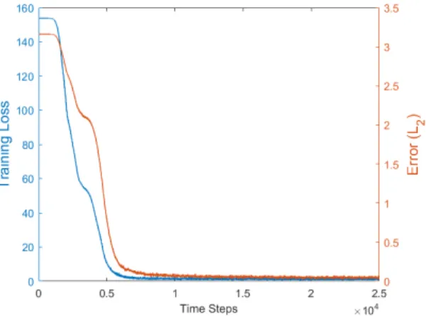
One cannot chooseψ(w) = kwk1, since it is neither differentiable nor strictly convex. However, ψ(w) = kwk1+, for any > 0, can be used. Figure 4 shows a compressed sensing example,
withn = 50,m = 100, and sparsityk = 10. SMD was used with a step size ofη = 0.001and the potential function wasψ(·) = k · k1.1. SMD converged to the true sparse solution after around
10,000 iterations. On this example, it was an order of magnitude faster than standardl1optimization.
Figure 2: The training loss and actual error of stochastic mirror descent for compressed sensing. SMD recovers the actual sparse signal.
Next we establishconvergence to the regularized pointfor the convex case. Proposition 9. Consider the following two cases.
(i) l(·)is differentiable and convex and has a unique root at 0,ψ(·)is strictly convex, and η >0is such thatψ−ηLiis convex for alli.
(ii) l(·)is differentiable and quasi-convex,l0(·)is zero only at zero,ψ(·)isα-strongly convex, and0< η≤mini
α|yi−xTiwi−1|
kxik2|l0(yi−xTiwi−1)|.
If either (i) or (ii) holds, then for anyw0, the SMD iterates given in Eq.(15)converge to w∞= arg min
w∈W
Dψ(w, w0). (29)
The proof is provided in Appendix C.
5.2 DISCUSSION OFHIGHLYOVER-PARAMETERIZEDNONLINEARMODELS
Let us consider the highly-overparameterized nonlinear model
yi =f(xi, w), i= 1, . . . , n, w∈Rm (30) where by highly-overparameterized we meanmn. Since the model is highly over-parameterized, it is assumed that we can perfectly interpolate the data points(xi, yi)so that the noiseviis zero. In
this case, the set of parameter vectors that interpolate the data is given byW ={w∈ Rm | y i =
f(xi, w), i= 1, . . . , n}, and Eq. (19), again, reduces to
Dψ(w, w0) =Dψ(w, wT) + T
X
i=1
for allw∈ W. Our proofs of convergence and implicit regularization for SGD and SMD in the linear case relied on two facts: (i)DLi(w, wi−1)was non-negative (this allowed us to show convergence), and (ii)DLi(w, wi−1)was independent ofw(this allowed us to show implicit regularization). Un-fortunately, neither of these hold in the nonlinear case.
However, they do hold in alocalsense. In other words, (i)DLi(w, wi−1) ≥ 0 forwi−1 “close enough” tow (see Figure 3), and (ii)DLi(w, wi−1)is weakly dependent on wfor wi−1 “close enough.” (Both statements can be made precise.)
Figure 3: Non-negativity ofDLi(w, wi−1)forwi−1“close enough” tow.
Now define
w∗=argmin
w∈WDψ(w, w0). (32)
Then one can show the following result.
Theorem 10. There exists an >0, such that ifkw∗−w0k< , then for sufficiently small step size η >0:
1. SMD iterates converge to a pointw∞∈ W
2. kw∞−w∗k=o()
This shows that if the initial condition is close enough, then we have convergence to a pointw∞that
interpolates the data, and thatw∞is an order of magnitude closer tow∗(the implicitly regularized
solution) than the initialw0was. At first glance, this result seems rather dissatisfying. It relies on w0being close to the manifoldW which appears hard to guarantee. We would now like to argue that in deep learningw0being close toWis often the case.
In the highly-overparameterized regime,mn, and so the dimension of the manifoldWism−n, which is very large. Now if thexi are sufficiently random, then the tangent space toW atw∗
will be a randomly oriented affine subspace of dimensionm−n. This means that any randomly chosen w0 will whp have a very large component when projected ontoW. In particular, it can be shown thatkw∗ −w0k2 = O(mn)· ky −f(x, w)k2, where y = vec(yi, i = 1, . . . , n)and
f(x, w) = vec(f(xi, w), i = 1, . . . , n). Thus, we may expect that, whenm n, the distance
of any randomly chosenw0 toW will be small and so SMD will converge to a point onW that approximately performs implicit regularization.
The gist of the argument is that (i) Whenm n, any random initial condition is “close” to the n−mdimensional solution manifoldW, (ii) whenw0is “close” tow∗, then SMD converges to a
pointw∞ ∈ W, (iii)w∞is “an order of magnitude closer” tow∗thanw0was, and (iv) thus, when
highly overparamatrized, SMD converges to a point that exhibits implicit regularization.
Of course, this was a very heuristic argument that merits a much more careful analysis. But it is suggestive of the fact that SGD and SMD, when performed on highly-overparameterized nonlinear models, as occurs in deep learning, may exhibit implicit regularization.
6
C
ONCLUDINGR
EMARKSWe should remark that all the results stated throughout the paper extend to the case of time-varying step sizeηi, with minimal modification. In particular, it is easy to show that in this case, the identity
(the counterpart of Eq. (19)) becomes
Dψ(w, w0) + T X i=1 ηil(vi) =Dψ(w, wT) + T X i=1 (Ei(wi, wi−1) +ηiDLi(w, wi−1)), (33)
whereEi(wi, wi−1) =Dψ(wi, wi−1)−ηiDLi(wi, wi−1) +ηiLi(wi). As a consequence, our main result will be the same as in Theorem 6, with the only difference that the small-step-size condition in this case is the convexity ofψ(w)−ηiLi(w)for alli, and the SMD with time-varying step size
will be the optimal solution to the following minimax problem
min {wi} max w,{vi} Dψ(w, wT) +P T i=1ηiDLi(w, wi−1) Dψ(w, w0) +P T i=1ηil(vi) . (34)
Similarly, the convergence and implicit regularization results can be proven under the same condi-tions (See Appendix D for more details on the time-varying case).
This paper opens up a variety of important directions for future work. Most of the analysis devel-oped here is general, in terms of themodel, theloss function, and thepotential function. Therefore, it would be interesting to study the implications of this theory for specific classes of models (such as different neural networks), specific losses, and specific mirror maps (which induce different reg-ularization biases). Something for future work.
R
EFERENCESAlessandro Achille and Stefano Soatto. On the emergence of invariance and disentangling in deep representations. arXiv preprint arXiv:1706.01350, 2017.
Tamer Bas¸ar and Pierre Bernhard.H-infinity optimal control and related minimax design problems: a dynamic game approach. Springer Science & Business Media, 2008.
Amir Beck and Marc Teboulle. Mirror descent and nonlinear projected subgradient methods for convex optimization.Operations Research Letters, 31(3):167–175, 2003.
Nicolo Cesa-Bianchi, Pierre Gaillard, G´abor Lugosi, and Gilles Stoltz. Mirror descent meets fixed share (and feels no regret). InAdvances in Neural Information Processing Systems, pp. 980–988, 2012.
Pratik Chaudhari and Stefano Soatto. Stochastic gradient descent performs variational inference, converges to limit cycles for deep networks. InInternational Conference on Learning Represen-tations, 2018.
John Duchi, Elad Hazan, and Yoram Singer. Adaptive subgradient methods for online learning and stochastic optimization.Journal of Machine Learning Research, 12(Jul):2121–2159, 2011.
Bruce A Francis.A course in H-infinity control theory. Berlin; New York: Springer-Verlag, 1987.
Claudio Gentile. The robustness of the p-norm algorithms. Machine Learning, 53(3):265–299, 2003.
Adam J Grove, Nick Littlestone, and Dale Schuurmans. General convergence results for linear discriminant updates.Machine Learning, 43(3):173–210, 2001.
Suriya Gunasekar, Blake E Woodworth, Srinadh Bhojanapalli, Behnam Neyshabur, and Nati Srebro. Implicit regularization in matrix factorization. InAdvances in Neural Information Processing Systems, pp. 6152–6160, 2017.
Suriya Gunasekar, Jason Lee, Daniel Soudry, and Nathan Srebro. Characterizing implicit bias in terms of optimization geometry.arXiv preprint arXiv:1802.08246, 2018a.
Suriya Gunasekar, Jason Lee, Daniel Soudry, and Nathan Srebro. Implicit bias of gradient descent on linear convolutional networks.arXiv preprint arXiv:1806.00468, 2018b.
Babak Hassibi and Thomas Kailath. Hoo optimal training algorithms and their relation to backprop-agation. InAdvances in Neural Information Processing Systems 7, pp. 191–198. 1995.
Babak Hassibi, Ali H. Sayed, and Thomas Kailath. Hoo optimality criteria for LMS and backprop-agation. InAdvances in Neural Information Processing Systems 6, pp. 351–358. 1994.
Babak Hassibi, Ali H Sayed, and Thomas Kailath. Hoo optimality of the LMS algorithm. IEEE Transactions on Signal Processing, 44(2):267–280, 1996.
Babak Hassibi, Ali H Sayed, and Thomas Kailath. Indefinite-Quadratic Estimation and Control: A Unified Approach to H2 and H-infinity Theories, volume 16. SIAM, 1999.
Elad Hazan. Introduction to online convex optimization. Foundations and Trends in Optimization, 2(3-4):157–325, 2016. ISSN 2167-3888.
Kenji Kawaguchi. Deep learning without poor local minima. InAdvances in Neural Information Processing Systems, pp. 586–594, 2016.
Diederik P Kingma and Jimmy Ba. Adam: A method for stochastic optimization. arXiv preprint arXiv:1412.6980, 2014.
Jyrki Kivinen, Manfred K Warmuth, and Babak Hassibi. The p-norm generalization of the LMS al-gorithm for adaptive filtering.IEEE Transactions on Signal Processing, 54(5):1782–1793, 2006.
Alex Krizhevsky, Ilya Sutskever, and Geoffrey E Hinton. Imagenet classification with deep convo-lutional neural networks. InAdvances in Neural Information Processing Systems, pp. 1097–1105, 2012.
Yann LeCun, Yoshua Bengio, and Geoffrey Hinton. Deep learning. Nature, 521(7553):436, 2015.
Jason D Lee, Max Simchowitz, Michael I Jordan, and Benjamin Recht. Gradient descent only converges to minimizers. InConference on Learning Theory, pp. 1246–1257, 2016.
Cong Ma, Kaizheng Wang, Yuejie Chi, and Yuxin Chen. Implicit regularization in nonconvex sta-tistical estimation: Gradient descent converges linearly for phase retrieval, matrix completion and blind deconvolution.arXiv preprint arXiv:1711.10467, 2017.
Siyuan Ma, Raef Bassily, and Mikhail Belkin. The power of interpolation: Understanding the effec-tiveness of SGD in modern over-parametrized learning. InProceedings of the 35th International Conference on Machine Learning, volume 80, pp. 3325–3334. PMLR, 2018.
Volodymyr Mnih, Koray Kavukcuoglu, David Silver, Andrei A Rusu, Joel Veness, Marc G Belle-mare, Alex Graves, Martin Riedmiller, Andreas K Fidjeland, Georg Ostrovski, et al. Human-level control through deep reinforcement learning.Nature, 518(7540):529, 2015.
Arkadii Nemirovskii, David Borisovich Yudin, and Edgar Ronald Dawson. Problem complexity and method efficiency in optimization. 1983.
Behnam Neyshabur, Ryota Tomioka, Ruslan Salakhutdinov, and Nathan Srebro. Geometry of opti-mization and implicit regularization in deep learning.arXiv preprint arXiv:1705.03071, 2017. Shai Shalev-Shwartz. Online learning and online convex optimization. Foundations and Trends in
Machine Learning, 4(2):107–194, 2012. ISSN 1935-8237.
Ravid Shwartz-Ziv and Naftali Tishby. Opening the black box of deep neural networks via informa-tion.arXiv preprint arXiv:1703.00810, 2017.
David Silver, Aja Huang, Chris J Maddison, Arthur Guez, Laurent Sifre, George Van Den Driessche, Julian Schrittwieser, Ioannis Antonoglou, Veda Panneershelvam, Marc Lanctot, et al. Mastering the game of go with deep neural networks and tree search.Nature, 529(7587):484–489, 2016. Dan Simon. Optimal state estimation: Kalman, H infinity, and nonlinear approaches. John Wiley
& Sons, 2006.
Mahdi Soltanolkotabi, Adel Javanmard, and Jason D Lee. Theoretical insights into the optimiza-tion landscape of over-parameterized shallow neural networks.arXiv preprint arXiv:1707.04926, 2017.
Daniel Soudry, Elad Hoffer, Mor Shpigel Nacson, Suriya Gunasekar, and Nathan Srebro. The im-plicit bias of gradient descent on separable data. arXiv preprint arXiv:1710.10345, 2017.
Tijmen Tieleman and Geoffrey Hinton. Lecture 6.5-rmsprop: Divide the gradient by a running average of its recent magnitude. COURSERA: Neural networks for machine learning, 4(2):26– 31, 2012.
Ashia C Wilson, Rebecca Roelofs, Mitchell Stern, Nati Srebro, and Benjamin Recht. The marginal value of adaptive gradient methods in machine learning. In Advances in Neural Information Processing Systems, pp. 4151–4161, 2017.
Yonghui Wu, Mike Schuster, Zhifeng Chen, Quoc V Le, Mohammad Norouzi, Wolfgang Macherey, Maxim Krikun, Yuan Cao, Qin Gao, Klaus Macherey, et al. Google’s neural machine trans-lation system: Bridging the gap between human and machine transtrans-lation. arXiv preprint arXiv:1609.08144, 2016.
Chiyuan Zhang, Samy Bengio, Moritz Hardt, Benjamin Recht, and Oriol Vinyals. Understanding deep learning requires rethinking generalization.arXiv preprint arXiv:1611.03530, 2016.
Zhengyuan Zhou, Panayotis Mertikopoulos, Nicholas Bambos, Stephen Boyd, and Peter W Glynn. Stochastic mirror descent in variationally coherent optimization problems. InAdvances in Neural Information Processing Systems, pp. 7043–7052, 2017.
Supplementary Material
A
P
ROOF OFL
EMMA4
Proof. Let us start by expanding the Bregman divergenceDψ(w, wi)based on its definition
Dψ(w, wi) =ψ(w)−ψ(wi)− ∇ψ(wi)T(w−wi).
By plugging the SMD update rule∇ψ(wi) = ∇ψ(wi−1)−η∇Li(wi−1)into this, we can write it as
Dψ(w, wi) =ψ(w)−ψ(wi)− ∇ψ(wi−1)T(w−wi) +η∇Li(wi−1)T(w−wi). (35)
Using the definition of Bregman divergence for(w, wi−1)and(wi, wi−1), i.e.,Dψ(w, wi−1) = ψ(w) − ψ(wi−1) − ∇ψ(wi−1)T(w − wi−1) and Dψ(wi, wi−1) = ψ(wi) − ψ(wi−1) −
∇ψ(wi−1)T(wi−wi−1), we can express this as
Dψ(w, wi) =Dψ(w, wi−1) +ψ(wi−1) +∇ψ(wi−1)T(w−wi−1)−ψ(wi)
− ∇ψ(wi−1)T(w−wi) +η∇Li(wi−1)T(w−wi) (36)
=Dψ(w, wi−1) +ψ(wi−1)−ψ(wi) +∇ψ(wi−1)T(wi−wi−1)
+η∇Li(wi−1)T(w−wi) (37)
=Dψ(w, wi−1)−Dψ(wi, wi−1) +η∇Li(wi−1)T(w−wi). (38)
Expanding the last term usingw−wi= (w−wi−1)−(wi−wi−1), and following the definition ofDLi(., .)from (16) for(w, wi−1)and(wi, wi−1), we have
Dψ(w, wi) =Dψ(w, wi−1)−Dψ(wi, wi−1) +η∇Li(wi−1)T(w−wi−1) −η∇Li(wi−1)T(wi−wi−1) (39) =Dψ(w, wi−1)−Dψ(wi, wi−1) +η(Li(w)−Li(wi−1)−DLi(w, wi−1)) −η(Li(wi)−Li(wi−1)−DLi(wi, wi−1)) (40) =Dψ(w, wi−1)−Dψ(wi, wi−1) +η(Li(w)−DLi(w, wi−1)) −η(Li(wi)−DLi(wi, wi−1)) (41) DefiningEi(wi, wi−1) := Dψ(wi, wi−1)−ηDLi(wi, wi−1) +ηLi(wi), we can write the above equality as
Dψ(w, wi) =Dψ(w, wi−1)−Ei(wi, wi−1) +η(Li(w)−DLi(w, wi−1)). (42) Notice that for any model class with additive noise, and any loss functionLithat depends only on
the residual (i.e. the difference between the prediction and the true label), the termLi(w)depends
only on the noise term, for any “true” parameter w. In other words, for allw that satisfyyi =
f(xi, w) +vi, we haveLi(w) =l(yi−f(xi, w)) =l(yi−(yi−vi)) =l(vi). Finally, reordering
the terms leads to
Dψ(w, wi) +ηDLi(w, wi−1) +Ei(wi, wi−1) =Dψ(w, wi−1) +ηl(vi), (43) which concludes the proof.
B
P
ROOF OFT
HEOREM6
Proof. We prove the theorem in two parts. First, we show that the value of the minimax is at least
1. Then we prove that the values is at most1, and is achieved by stochastic mirror descent for small enough step size.
1. Consider the maximization problem
max w,{vi} Dψ(w, wT) +ηPTi=1DLi(w, wi−1) Dψ(w, w0) +ηP T i=1l(vi) .
Clearly, the optimal solution and the optimal values of this problem can, and will, be a function of{wi}. Similarly, we can also choose feasible points that depend on{wi}. Any
choice of a feasible point( ˆw,{vˆi})gives a lower bound on the value of the problem. Before
choosing a feasible point, let us first expand the DLi(w, wi−1)term in the numerator, according to its definition.
DLi(w, wi−1) =l(vi)−l(yi−fi(wi−1))+l 0(y
i−fi(wi−1))∇f(wi−1)T(w−wi−1), (44) where we have used the fact thatl(yi−fi(w)) =l(vi)for all consistentw, in the first term.
Now, we choose a feasible point as follows
ˆ
vi=fi(wi−1)−fi( ˆw), (45)
wherewˆ is the choice ofw, as will be described soon. The reason for choosing this value for the noise is that it “fools” the estimator by making its loss on the corresponding data point zero. In other words, for this choice, we have
DLi(w, wi−1) =l(ˆvi)−l(0) +l
0(0)∇f(w
i−1)T( ˆw−wi−1)
=l(ˆvi)
becausel(0) =l0(0) = 0. It should be clear at this point that this choice makes the second
terms in the numerator and the denominator equal, independent of the choice ofw. Whatˆ
remains to do, in order to show the1lower-bound, is to take care of the other two terms, i.e.,Dψ(w, wT)andDψ(w, w0). As we would like to make the ratio equal to one, we
would like to haveDψ(w, wT) =Dψ(w, w0), which is equivalent to having
ψ(w)−ψ(wT)− ∇ψ(wT)T(w−wT) =ψ(w)−ψ(w0)− ∇ψ(w0)T(w−w0)
which is, in turn, equivalent to
(∇ψ(wT)− ∇ψ(w0)) T
w=−ψ(wT) +ψ(w0) +∇ψ(wT)TwT − ∇ψ(w0)Tw0. (46)
Since∇ψis an invertible function,∇ψ(wT)− ∇ψ(w0)6= 0, ifwT 6=w0. Therefore, the
above equation has a solution forw, ifwT 6=w0. As a result, choosingwˆto be a solution
to (46) makesDψ( ˆw, wT) = Dψ( ˆw, w0), ifwT 6=w0. For the case whenwT = w0, it
is trivial thatDψ( ˆw, wT) = Dψ( ˆw, w0)for any choice ofw. In this case, we only needˆ to choose wˆ to be different fromw0, to avoid making the ratio 00. Hence, we have the following choice
ˆ
w=
a solution of (46) forwT 6=w0
w0+δw for someδw6= 0 forwT =w0
(47)
Choosing the feasible pointw,ˆ {vi}according to (47) and (45) leads to
max w,{vi} Dψ(w, wT) +ηPTi=1DLi(w, wi−1) Dψ(w, w0) +ηP T i=1l(vi) ≥ Dψ( ˆw, wT) +η PT i=1l(fi(wi−1)−fi( ˆw)) Dψ( ˆw, w0) +ηP T i=1l(fi(wi−1)−fi( ˆw)) . (48)
Taking the minimum of both sides with respect to{wi}, we have
min {wi} max w,{vi} Dψ(w, wT) +ηP T i=1DLi(w, wi−1) Dψ(w, w0) +ηP T i=1l(vi) ≥min {wi} Dψ( ˆw, wT) +ηP T i=1l(fi(wi−1)−fi( ˆw)) Dψ( ˆw, w0) +ηPTi=1l(fi(wi−1)−fi( ˆw)) = 1. (49)
The equality to1comes from the fact the that the optimal solution of the minimization either hasw∗
2. Now we prove that, under the small step size condition (convexity ofψ(w)−ηLi(w)for
alli), SMD makes the minimax value at most1, which means that it is indeed an optimal solution. Recall from Lemma 5 that
Dψ(w, w0) +η T X i=1 l(vi) =Dψ(w, wT) + T X i=1 Ei(wi, wi−1) +η T X i=1 DLi(w, wi−1), where Ei(wi, wi−1) =Dψ(wi, wi−1)−ηDLi(wi, wi−1) +ηLi(wi).
It is easy to check that whenψ(w)−ηLi(w)is convex,Dψ(wi, wi−1)−ηDLi(wi, wi−1) is in fact a Bregman divergence (i.e. the Bregman divergence with respect to the potential ψ(w)−ηLi(w)), and therefore it is nonnegative for anywiandwi−1. Furthermore, we
know that the lossLi(wi)is also nonnegative for allwi. It follows thatEi(wi, wi−1)is nonnegative for all values ofwi, wi−1andi. As a result, we have the following bound.
Dψ(w, w0) +η T X i=1 l(vi)≥Dψ(w, wT) +η T X i=1 DLi(w, wi−1). (50)
Since the Bregman divergenceDψ(w, w0)and the lossl(vi)are nonnegative, the left-hand
side expression is nonnegative, and it follows that
Dψ(w, wT) +ηP T i=1DLi(w, wi−1) Dψ(w, w0) +ηP T i=1l(vi) ≤1. (51)
In fact, this means that independent of the choice of the maximizer (i.e. for all{vi}and
w), as long as the step size condition is met, SMD makes the ratio less than or equal to1.
Combining the results of 1 and 2 above concludes the proof.
B.1 PROOF OFTHEOREM3
Proof. This result is a special case of Theorem 6, which was proven above. In this case,ψ(w) =
1 2kwk 2,f(x i, w) =xTi w, andl(z) = 1 2z 2. Therefore,D ψ(w, wT) = 12kw−wTk2,Dψ(w, w0) = 1 2kw−w0k 2,D Li(w, wi−1) = 1 2(x T
iw−xTiwi−1)2, andl(vi) = 12v2i, which leads to the result.
C
P
ROOF OFP
ROPOSITION9
Proof. To prove convergence, we appeal again to Equation (22), i.e.
Dψ(w, w0) =Dψ(w, wT) + T
X
i=1
(Ei(wi, wi−1) +ηDLi(w, wi−1)), (52)
for allw∈ W. We prove the two cases separately.
1. The proof of case (i) is straightforward. When l(·) is differentiable and convex, Li is
also convex, and therefore DLi(w, wi−1) is nonnegative. Moreover, when ψ−ηLi is convex,Ei(wi, wi−1)is also nonnegative. Therefore, the entire summand in Eq. (52) is nonnegative, and has to go to zero fori → ∞. That is because as T → ∞, the sum should remain bounded, i.e.,P∞
i=1(Ei(wi, wi−1) +ηDLi(w, wi−1)) ≤Dψ(w, w0). As a result of the non-negativity of both terms in the sum, we have bothEi(wi, wi−1) → 0 andDLi(w, wi−1) → 0asi → ∞, which imply Li(wi−1) → 0. This implies that the updates in (15) vanish and we get convergence, i.e.,w → w∞. Further, again because
Li(wi−1)→0, and 0 is the unique root ofl(·), all the data point are being fit, which means w∞∈ W.
2. To prove case (ii), note that we have DLi(w, wi−1) =Li(w)−Li(wi−1)− ∇Li(wi−1) T(w−w i−1) (53) = 0−l(yi−xTiwi−1) +l0(yi−xTiwi−1)xiT(w−wi−1) (54) =−l(yi−xTi wi−1) +l0(yi−xTiwi−1)(yi−xTiwi−1), (55) and Ei(wi, wi−1) =Dψ(wi, wi−1)−ηDLi(wi, wi−1) +ηLi(wi) (56) =Dψ(wi, wi−1) +η Li(wi−1) +∇Li(wi−1)T(wi−wi−1) (57) =Dψ(wi, wi−1) +η l(yi−xTi wi−1)−l0(yi−xTiwi−1)xTi (wi−wi−1) . (58) It follows from (55) and (58) that the summand in Equation (52) is
Ei(wi, wi−1) +ηDLi(w, wi−1) =Dψ(wi, wi−1) +ηl 0(y
i−xTiwi−1)(yi−xTiwi).
(59) The first term is a Bregman divergence, and is therefore nonnegative. In order to establish convergence, one needs to argue that the second term is nonnegative as well, so that the summand goes to zero asi→ ∞. Sincel(·)is increasing for positive values and decreasing for negative values, it is enough to show thatyi−xTi wi−1andyi−xTiwihave the same sign,
in order to establish nonnegativity. It is not hard to see that if the distance between the two points is less than or equal to the distance ofyi−xTi wifrom the origin, then the signs are the
same. In other words, if|(yi−xTiwi)−(yi−xTiwi−1)|=|xTi(wi−wi−1)| ≤ |yi−xTiwi−1|, then the sign are the same.
Note that by the definition ofα-strong convexity ofψ(·), we have
(∇ψ(wi)− ∇ψ(wi−1))T(wi−wi−1)≥αkwi−wi−1k2, (60) which implies
−η∇Li(wi−1)T(wi−wi−1)≥αkwi−wi−1k2, (61) by substituting from the SMD update rule. Upper-bounding the left-hand side by ηk∇Li(wi−1)kk(wi−wi−1)kimplies
ηk∇Li(wi−1)k ≥αkwi−wi−1k. (62) This implies that we have the following bound
|xTi (wi−wi−1)| ≤ kxikkwi−wi−1k ≤
ηkxikk∇Li(wi−1)k
α . (63)
It follows that if η ≤ α|yi−xTiwi−1|
kxikk∇Li(wi−1)k, for all i, then the signs are the same, and the
summand in Eq.(52) is indeed nonnegative. This condition can be equivalently expressed as η≤ α|yi−xTiwi−1|
kxik2|l0(yi−xTiwi−1)|for alli, orη≤mini
α|yi−xTiwi−1|
kxik2|l0(yi−xTiwi−1)|, which is the condition in the statement of the proposition.
Now that we have argued that the summand is nonnegative, the convergence tow∞∈ Wis
immediate. The reason is that bothDψ(wi, wi−1)→0andl0(yi−xTiwi−1)(yi−xTiwi)→
0, asi → ∞. The first one implies convergence to a pointw∞. The second one implies
that eitheryi−xTiwi−1= 0oryi−xTiwi= 0, which, in turn, impliesw∞∈ W.
D
T
IME-V
ARYINGS
TEP-S
IZEThe update rule for the stochastic mirror descent with time-varying step size is as follows. wi= arg min
w
ηiwT∇Li(wi−1) +Dψ(w, wi−1), (64)
which can be equivalently expressed as∇ψ(wi) =∇ψ(wi−1)−ηi∇Li(wi−1), for alli. The main results in this case are as follows.
Lemma 11. For any (nonlinear) modelf(·,·), any differentiable lossl(·), any parameterw and noise values{vi}that satisfyyi = f(xi, w) +vifori = 1, . . . , n, any initializationw0, any step
size sequence{ηi}, and any number of stepsT ≥ 1, the following relation holds for the SMD
iterates{wi}given in Eq.(64)
Dψ(w, w0) + T X i=1 ηil(vi) =Dψ(w, wT) + T X i=1 (Ei(wi, wi−1) +ηiDLi(w, wi−1)), (65)
Proof. The proof is straightforward by summing the following equation for alli= 1, . . . , T Dψ(w, wi−1) +ηil(vi) =Dψ(w, wi) +Ei(wi, wi−1) +ηiDLi(w, wi−1), (66) which can be easily shown in the same way as in the proof of Lemma 4 in Appendix A.
Theorem 12. Consider any general model f(·,·), and any differentiable loss functionl(·)with propertyl(0) = l0(0) = 0. For sufficiently small step size, i.e., for any sequence{ηi}for which
ψ(w)−ηiLi(w)is convex for alli, the SMD iterates{wi}given by Eq.(64)are the optimal solution
to the following minimization problem
min {wi} max w,{vi} Dψ(w, wT) +P T i=1ηiDLi(w, wi−1) Dψ(w, w0) +PTi=1ηil(vi) . (67)
Furthermore, the optimal value (achieved by SMD) is1.
Proof. The proof is similar to that of Theorem 6, as presented in Appendix B. The argument for the upper-bound of1is exactly the same. For the second part of the proof, we use the previous Lemma. It follows from the convexity ofψ(w)−ηiLi(w)thatEi(wi, wi−1)≥0, and as a result we have
Dψ(w, wT) +P T
i=1ηiDLi(w, wi−1) Dψ(w, w0) +PTi=1ηil(vi)
≤1 (68)
for SMD updates, which concludes the proof.
The convergence and implicit regularization results hold similarly, and can be formally stated as follows.
Proposition 13. Consider the following two cases.
(i) l(·)is differentiable and convex and has a unique root at 0,ψ(·)is strictly convex, and the positive sequence{ηi}is such thatψ−ηiLiis convex for alli.
(ii) l(·)is differentiable and quasi-convex and has zero derivative only at 0,ψ(·)isα-strongly convex, and0< ηi≤ α|yi−x
T iwi−1|
kxik2|l0(yi−xTiwi−1)|for alli.
If either (i) or (ii) holds, then for any initializationw0, the SMD iterates given in Eq.(64)converge to
w∞= arg min
w∈W
Dψ(w, w0). (69)