An estimated new Keynesian dynamic stochastic general equilibrium model of the Euro area

EUROPEAN

ECONOMY

EUROPEAN COMMISSION

ECONOMIC

PAPERS

ISSN 1725-3187

http://europa.eu.int/comm/economy_finance

N° 220 January 2005 An estimated new keynesian dynamic stochastic

general equilibrium model of the Euro area by

Marco Ratto**, Werner Röger*, Jan in’t Veld* and Riccardo Girardi**

*Directorate-General for Economic and Financial Affairs ** Joint Research Centre

Economic Papers

are written by the Staff of the Directorate-General for Economic

and Financial Affairs, or by experts working in association with them. The "Papers"

are intended to increase awareness of the technical work being done by the staff and

to seek comments and suggestions for further analyses. Views expressed represent

exclusively the positions of the author and do not necessarily correspond to those of

the European Commission. Comments and enquiries should be addressed to the:

European Commission

Directorate-General for Economic and Financial Affairs

Publications

BU1 - -1/180

B - 1049 Brussels, Belgium

ECFIN/007878/04-EN

ISBN

92-894-8119-6

KC-AI-04-220-EN-C

Table of contents

1 Introduction ... 3

2 The DSGE Model... 5

3 Estimation Methodology ... 11

3.1 Solving the model with linear approximations... 12

3.2 Maximum likelihood estimation and inference... 13

3.3 Bayesian estimation and inference ... 14

3.3.1 Implementation: MCMC (Metropolis-Hastings)... 14

3.4 Model comparison... 16

4 Estimation... 17

4.1 Prior distributions ... 17

4.2 Parameter estimates and shocks identified... 21

4.3 VAR comparison... 25

5 Which structural shocks drive the euro economy?... 26

6 Estimated impulse responses of structural shocks ... 29

7 Conclusions ... 39

8 References ... 40

Annex: ... 41

A1. Results from posterior maximization ... 41

1 Introduction

In recent years a new consensus has emerged in macroeconomics in general and in model building in particular, the so called New Keynesian Paradigm (NKM). This paradigm is well established as can be seen from the prominent treatment in recent textbooks (see, for example Obstfeld/Rogoff) and literature surveys (se for example Clarida, Gali Gertler). In a sense the NKM paradigm combines elements from the RBC literature with more traditional Keynesian ideas. Traditional Keynesian models suffered from underdeveloped microfoundations and a lack of long term factors influencing the economy which made them subject to the Lucas critique. It also did not have a coherent theoretical explanation for the sluggish behaviour of prices it assumed. On the other hand, RBC modellers built their models up from the actions of optimising economic agents whose choices are made within specified constraints. The New Classical view of RBC modellers saw business cycles as largely the result of shocks to productivity and preferences, and downturns as merely the optimal adjustment of the economy to such disturbances. NKM models correct the RBC models by introducing frictions in goods, labour and financial markets in order to provide a better fit with actual data, but at the same time tries to model the frictions explicitly as constraints faced by households and firms. This allows combining optimal behaviour with rigidities in a way which avoids the Lucas critique.

The QUEST model has been set up in the spirit of a NKM model, with a strong emphasis on theoretical consistency of the behavioural equations. However at the time when QUEST II was introduced the estimation technology for DSGE models was not sufficiently developed to allow for rigorous estimation and testing of these models. Large parts of these models needed to be calibrated. Following recent developments in Bayesian estimation techniques (see, e.g., Geweke 1999 and Schorfheide 2000), it has become possible to estimate these type of models. Smets and Wouters (2003) have been the first to estimate such a model for the Euro area. They followed Cristiano, Eichenbaum, and Evans (2001) and designed a DSGE model for the Euro area featuring price and wage stickiness, partial indexation of prices and salaries, external capital formation, variable capital utilisation rate and stochastic shocks to each structural equation of the resulting model. Smets and Wouters (2003) show that the current generation of New-Keynesian DSGE models is sufficiently rich to capture the time-series properties of the data, as long as a sufficient number of structural shocks is considered. In particular, it is able to match the degree of empirical persistence found in the euro area data for inflation and wages quite well.

This paper applies Bayesian estimation techniques to a time series data set of the euro area and presents estimates of a DSGE model. The purpose of this paper is not to estimate the current version of the QUEST model directly with these methods but rather to estimate a prototype new generation New-Keynesian DSGE model. This model can then serve as a benchmark for an estimation of a QUEST specification. In fact in some dimensions the QUEST model may need to be adjusted to come closer to a DSGE model.

One of the common features between the QUEST II model and the estimated New-Keynesian DSGE model presented in this paper are that both, in the long run, closely resemble the standard neoclassical growth model. All behavioural relations are derived from dynamic optimisation problems of households and firms, with optimisation subject to technological constraints, budget constraints and/or institutional constraints, often captured as adjustment

costs. This leads to a description of economic behaviour that is a mixture of backward and forward looking behaviour. The main differences with the QUEST II model are in the specification of consumption. While consumption in the QUEST model is based on a permanent income model for finitely-lived households, as popularised by Blanchard (1984), in this DSGE model in contrast, consumption is derived from intertemporal optimisation for infinitely lived households, like in all other current DSGE models. However, consumption is modelled more backward looking by allowing for habit persistence (i.e. consumption decisions today depend partially on the previous pattern of consumption). On the other hand, QUEST allowed for liquidity constraints, a feature still missing in the consumption framework here. The differences in the investment specification are only of minor importance, with a stronger emphasis on adjustment costs here. The modelling of the labour market is substantially different. Here, like in other DSGE models, this is based on a neoclassical labour supply with monopoly power for workers. One of the distinguishing features of the QUEST model is the labour market specification derived from a theoretical search model based on the work by Pissarides (1990).

The estimated model as presented here is still incomplete since it treats the Euro area as a closed economy. The closed economy setting was chosen because we first wanted to concentrate on the main aggregates consumption and investment as well as on prices and wages and their interactions. However, adding a trade sector would be among our first priorities for further extensions of this model. The model will then include a more explicit modelling of trade frictions within the framework of convex adjustment costs, which would distinguish it from the QUEST model, where trade is modelled through an ad-hoc specification of adjustment lags in quantities and prices.

An important reason for estimating a DSGE model was also to be able to compare estimation results with the existing literature and to make sure that the estimation yields results which are consistent with the results obtained with similar specifications and similar datasets.

The main goals of this exercise are:

1) Demonstrate that models derived from economic theory can fit Euro area data, provided one allows for sufficient institutional restrictions. We compare the predictive performance of the estimated DSGE model with that of a VAR model estimated over the same euro area data set. (We intend to conduct a similar exercise for the US economy to see whether institutional constraints play the same role there).

2) Identify the main structural shocks hitting the Euro area economy in a theoretically consistent way. An advantage of an explicit structural model is the fact that residuals can be given a structural interpretation, i.e. we can identify shocks which originate from consumption, technology, labour supply, labour demand, investment and fiscal and monetary policy. This may be of added value in trying to understand the nature of the current economic situation. For example, the model identifies a declining trend in government spending, which is reversed in recent years, a decline in price mark-ups, reflecting increased competitive pressures, a trend increase in total factor productivity in the 1980s, followed by a decline in the late 1990s and a trend increase in labour supply, reflecting a declining NAIRU.

3) Provide the typical response of the economy to the individual shocks in the form of impulse responses, like in VAR studies, with the additional benefit that confidence intervals can be provided to show the uncertainty surrounding these responses.

The outline of the paper is as follows. Section 2 presents the model. In section 3 discusses the estimation methodology. Since estimation of these models is non standard a fairly comprehensive explanation will be provided. Section 4 presents the estimation results. In order to provide a more intuitive understanding for the quality of the fit of this model, a comparison with a simple VAR model is given. Section 5 presents and interprets the structural shocks identified by the model estimates and section 6 describes the dynamic adjustment of the euro area economy to structural shocks.

2 The DSGE Model

Households:

The household sector decides about consumption and asset accumulation (including fixed capital). Each household supplies a specific variety of labour in a monopolistically competitive fashion, i.e. the household sector sets the wage given the demand curve for labour. When making decisions the household also faces adjustment costs for changing wages. These adjustment costs are borne by the household (see budget constraint). The household maximises a utility function subject to a budget constraint. The Lagrangian of this maximisation problem is given by

(1)

(

)

∑

∑

The household maximises a utility function over consumption, leisure and real money balances. Following the recent literature we allow for habit persistence in consumption. This is an important modification w. r. t. the current consumption specification in QUEST which was based entirely on a pure life cycle model. The current version allows for lagged adjustment of consumption and we choose a logarithmic specification

(2a) ( )= log( i − _t−1) t C t i t C habC C U ε

where denotes a stochastic preference shock for consumption in period t. This specification yields the following expression for the marginal utility of consumption

C t ε (2b) ) ( 1 1 , − − = t i t C t i t C habC C U ε .

The consumption index is itself an aggregate over different goods which are imperfect substitutes. The preferences of households are expressed by a CES utility function

(2c) t t t dj C C i t i t τ τ τ − −       =

_∫

where τ_t measures the inverse of the time varying elasticity of demand of households for consumption goods of type j. The term τ_t is given by

(2d) τ_t =τ0 +τ1(Y_t −Ypot_t)+ε_tτ

where ετ_t is a autocorrelated shock to the demand elasticity. For labour supply we use a CES utility function

(2e) κ κ ω ε ₋ − − = − _{(1 )}1 1 ) 1 ( i t L t i t L L V with κ>0,

where is a possibly autocorrelated labour supply shock. The marginal utility of leisure is given by L t ε (2f) ₌₋ε ω_{(1− )}−κ. , tL it i t L L V

The household decides about consumption, asset accumulation and the supply of labour (or more correctly about wages) and real money holdings1. The first order conditions of the household (FOCs) with respect to consumption and financial wealth are given by the following equations: (3a) 0 _{=> , − =}0 ∂ ∂ t t t i t C i t P PC U C U _λ (3b) 1 1 0 1 1 0 _{=>− + =} ∂ ∂ + + t t t t t i t PR P B U _{λ λ β} (3c) 0 _{=> − =}0 ∂ ∂ ζ t i t t i t _{Y R} P M M U

The labour supply decision is slightly more complex, since it is assumed that workers have a certain market power in the labour market, because they offer services, which are imperfect substitutes to services offered by other workers. That means aggregate labour demand of firms is a composite of labour supplied by individual workers. Total employment in production is characterised by a CES function

1 _{With an interest rate rule as specified below, an optimality condition for money would only determine the}

desired money holdings of the household sector without any further consequence for the rest of the economy. For that reason any further discussion on money demand is dropped here.

(4a) 1 1 0 1 − −       =

∫

where the parameter θ determines the degree of substitutability between labour supplied by individual households. Corresponding to the CES aggregator there exists a wage index

(4b) −θ_ −θ      =

∫

This technology yields a labour demand equation as perceived by household i

(4c) _t t i t i t L W W L θ −       =

In a monopolistic labour market the elasticity of substitution between different types of labour is important for determining the mark-up of wages over the equilibrium wage. This elasticity is defined by (4d) _i t i t i t t t i t i t i t W L W L W W W L _θ θ _=−θ       − = ∂ ∂ − 1 .

Now the wage setting rule can be derived taking derivatives of the Lagrangian w.r.t. wages. Using symmetry: Wi _t and neglecting second order terms allows us to write

t =W (5a) W t w t W t w t t t L i t P W V W U 1 1 0 (1 ) + + +       − − − = => ∂ ∂ _{γ π λ βγ π} θ θ λ ,

where is the growth rate of nominal wages. This can be reformulated as a wage setting rule W t π (5b) w t t t t w t w w t _{P R} W mup L C 1 1 ) 1 ( ) 1 ( 1 + +       − − − = π ω γ π _κ with θ 1 − = w mup

where wage inflation is determined by the gap between the reservation wage and the real wage adjusted for a wage mark up. The forward looking nature of wage setting is reflected by the forward wage inflation term. This formulation generalises the neoclassical labour supply model along two dimensions. First, by introducing convex wage adjustment costs (γ_w >0), workers want to smooth wage adjustments, taking into account current and future expected labour market conditions. Second, because workers offer services which are imperfect substitutes to services offered by other workers, they can demand wages which are above their reservation wage2. The reservation wage is the marginal value of leisure, divided by the

marginal utility of consumption. That means for a given utility of leisure the reservation wage increases with a decline in the marginal utility of consumption that an additional unit of labour can buy. In estimating the wage rule two further generalisations have been introduced. Some search theoretic generalisations of the neoclassical wage rule suggest rules where wages are indexed to both the reservation wage and the marginal value product of labour with weight bg reflecting the bargaining strength of workers (see, for example, Shi et al. (1999)). In order to allow for backward looking behaviour it is assumed that only a fraction sfw of workers form rational expectations of future wages, while the remaining workers follow a simple rule of thumb where expectations are determined by past inflation. These two modifications lead to the following wage equation

(5c) (1 ) 1

(

)

There are N firms indexed by j. Because goods produced by individual firms are imperfect substitutes, firms are monopolistically competitive in the goods market and face a demand function for goods given by

(6) ( ) 1 t t t t j t j j t C G I P P s Y _ t + +      = − τ

Output is produced with a Cobb Douglas production function

(7) ( )1α( j)α t t j t j t j t ucap K U L Y ₌ −

with capital and labour as inputs. Firms can also decide about the degree of capacity utilisation The level of technology is subject to random technology shocks ( ) and follows the autoregressive process

U t ε (8) U. t U t U t U U U )=ρ log( ₋ )+(1−ρ )log( )+ε log( ₁

The objective of the firm is to maximise the present discounted value of its cash flows. Dynamic considerations enter the problem of the firm because firm faces quadratic costs of changing capital, employment and prices. Finally firms must also choose the optimal level of capacity utilisation.

[

]

[

]

[

]

∑

∑

∑

∏

is the discount factor, which consists of the short term interest rate and a risk premium (rp). The risk premium can be subject to random shocks and generated by the following autoregressive process

(10) rp t t rp t rp t rp rp rp =ρ ₋₁+(1−ρ ) ₋₁+ε

For adjustment costs we choose the following convex functional forms (11) 2 1 2 1 2 2 2 2 ) ( ) , ( 1 / , 2 ) ( 2 ) ( j t I t j t I t K j t j t K j t j t j t j t P j t P j t L j t t t W t j t L I K I I K adj P P with P adj L L P W L adj ∆ + + = − = ∆ = ∆ + = − − γ ε γ π π γ γ ε 2 2 1( *) ( *) )

(ucap a ucap ucap a ucap ucap

adj j t j t j t CAP _{= − + −}

The firm determines labour input, the capital stock, capacity utilisation and prices optimally in each period given the technological and administrative constraints as well as demand conditions. The first order conditions are given by:

(12a) 0 ( ₁ ) ( ₁) (1 W) t j t t j t j t L j t j t t L j t j t j t j t P W L L L L R L Y L V _{α η} γ _{γ = +ε}       − − − + => ∂ ∂ − + (12b) ( ) ( 1 ₁) 1 1 0 _{=> + + ∆ − ∆ = −} ∂ ∂ + − t j t j t I j t j t I t K j t q I R I K I I V _{γ ε γ} (12c) 1 2 2 2 1 1 2 0 _{(1 ) (( ) ( 2 ) ) (1 )} + − − − − = + − + − − − => ∂ ∂ t t t t j t j t t j t j t j t q rp r q ucap a ucap a a a a K Y K V _{α η δ} (12d) j t j t j t j t j t j t K ucap Y ucap a a a ucap V _{α η} ) 1 ( )) ( 2 ) 2 (( _{1 2 1} 0 _{=> − + = −} ∂ ∂

(12e)

[

]

Firms equate the marginal product of labour, net of adjustment costs, to wage costs. Wage costs include a stochastic wage cost shock. This should be seen as shocks to administrative burdens related to current employment. As can be seen from the left hand side of equation (12a), the convex part of the adjustment cost function penalises in cost terms accelerations and decelerations of changes in employment. Equations (12b-d) jointly determine the optimal capital stock and optimal capacity utilisation. The firm equates the marginal product of capital to the rental price of capital, adjusted for capital costs. The firm also equates the marginal product of capital services (K*ucap) to the marginal cost of capacity utilisation. Equation (12e) defines the mark up factor as a function of the elasticity of substitution and changes in inflation. We follow Smets and Wouters and allow for additional backward looking elements by assuming that a fraction (1-sfp) of firms keep prices fixed at the t-1 level. This leads to the following specification: (12e’)

[

]

The government sector and fiscal policy is treated in a rather rudimentary fashion. The share of government purchases (13a) G G t t t t /Y = gs +ε

fluctuates systematically with the business cycle according to the following rule (13b) Y( _{t t})

g

t t Y Ypot

gs = −

where measures the degree of automatic stabilisation of government expenditure. Discretionary fiscal action is characterised by the variable which is allowed to be autocorrelated process. Implicitly it is assumed that government expenditure is financed, by lump sum taxes.

Y g t G t ε

Central bank policy rule (interest rate rule):

Monetary policy is modelled via the following Taylor rule, which allows for some smoothness of the interest rate response to the inflation and output gap

(14a) M t t t t t Y M t t M t t Y M T t t M T t t t Ypot Y Ypot Y t t Ypot Y t t R Ex ilag inom ilag inom ε π π π π π π π + − − − + − + − + − + + − + = − − ∆ − ∆ − − )) ( ( ) ( ) ( ) ( . ( * ) 1 ( * 1 1 1 1 1

The term captures random discretionary shocks to monetary policy and is a time varying inflation target, specified as follows

M t ε T t π (14b) T T T T _t T. t T t ρπ π ρπ π επ π = ₋₁+(1− ) + T π

ε is an i.i.d. shock to the inflation target. It is assumed that both fiscal and monetary authorities base their policies on a concept of potential output which is a smooth function of past output

(15) Ypot_t =ρ_ypotYpot_t−1+(1−ρ_ypot)Y_t

3 Estimation

Methodology

We present the first attempt to apply a Bayesian estimation approach to bring the model directly to the data. This approach has been discussed by many authors in the literature in the last few years (e.g. Schorfheide 2000, Lubik and Schorfheide, 2003, Smets and Wouters, 2003). Schematically, the method consists of the following steps:

• the non-linear DSGE model is solved via a linear approximation: a linear rational expectation system is obtained that must be obtaining a ‘standard’ linear model in state space form;

• the state-space approximation of the original non-linear model allows the identification of a likelihood function (via e.g. Kalman recursions) and a subsequent inference based on it (maximum likelihood estimation, etc.);

• usually theoretical model imply few, well defined shocks; unfortunately this often implies singularities in the determination of the likelihood (in the Kalman filter the number of shocks must at least be as large as the number of observables), implying the introduction of additional structural shocks and/or measurement errors;

• likelihood-based inference presents a series of issues: specifically the lack of identification (global: multiple maxima; local: over-parameterisation, i.e. the maximum is given by a complex multidimensional combination/interaction structure rather then by a single point in the parameter space);

• the Bayesian analysis is performed: prior distributions for model parameters have to be defined, representing the prior beliefs of the analyst on their plausible values, which, in combination with the likelihood function, allows to obtain the posterior distribution;

• the Bayesian inference needs the use of stochastic simulations, specifically Markov Chain Monte Carlo (MCMC) techniques, allowing to obtain samples from the posterior joint pdf of the model parameters and subsequently to make an inference in which the parameter uncertainty and the shape of the likelihood are taken into account;

• the model is finally compared to an empirical model; in the literature this is usually a VAR model.

From the computational point of view, the linear approximation and the solution of the obtained LRE can be done automatically using the DYNARE program (Juillard, 1996, 2003), which applies the generalised Schur decomposition solution method (Klein, 2000). DYNARE is a software for the simulation of DSGE models, freely available and totally open source. Presently, an estimation module is implemented on DYNARE, to include the most recent developments in Bayesian estimation macro-economic models in an extremely efficient and easy way. DYNARE is also extremely flexible, and allows to easily incorporating problem specific methodological issues or customisations.

3.1 Solving the model with linear approximations

Let a model be defined and first order conditions identified. This can be expressed as: (16)

{

}

{ }

{

}

where y is vector of endogenous variables, ε is the vector of exogenous stochastic shocks, θ is the vector of parameters and E is the expectation operator.

The non-linear model is solved via a linear approximation around the deterministic steady state y such that f(y,y,y,0;θ)=0. A linear rational expectation (LRE) system is obtained, with forward looking components

(17) A+E_tyˆ_t+1+A0yˆ_t +A−yˆ_t−1+Bε_t =0, where yˆ_t =y_t−y

The system is solved for the reduced form state equation in its predetermined variables (Blanchard and Kahn, 1980; generalised Schur form, Klein, 2000). An observation equation is also added to link the observed variables y_t∗ to the predetermined ones, obtaining:

(18) ) ( ) ' ( ) ( ) ' ( ) ( ˆ ) ( ˆ ) ˆ ) ( ( 1 θ ε ε θ η η ε θ θ η θ Q E V E H y G y y y M y t t t t t t t t t t = = + = + + = − ∗

where η_t is the measurement error, if any. The system matrices G, H, V and Q and the steady state vector y(θ) are functions of the vector of structural parameters θ of the original model. Vector θ includes the noise parameters Σ. The state space representation (18) allows use of Kalman filtering for the computation of the log-likelihood, and a subsequent inference based on it (maximum likelihood estimation, etc.).

In the original model specification (16), well-defined (and relatively few) shocks are usually present. If the number of shocks is smaller than the number of observed variables, singularities in the Kalman filter will be present, i.e. the probability distribution of the observables (the likelihood) can be degenerate. This implies the introduction of additional shocks until the system becomes non-singular, including either measurement errors

) | (YT θ p

t

η (as e.g. in Ireland, 2004, who also models the measurement error as a VAR(1) process) or additional structural shocks in the state equation (as e.g. in Smets and Wouters, 2003). Rigorously, in such cases, as clearly stated by Schorfheide (2000), the evaluation approach here applied will “lead to an assessment of the modified model rather than the original one”. In such cases, the parameter vector θ will be augmented for the additional noise terms and, if any, also for the VAR coefficients in the measurement errors as in Ireland (2004). In this paper we follow the Smets and Wouters approach and introduce a sufficient number of structural shocks in the state equations.

3.2 Maximum likelihood estimation and inference

The state space form of the linear approximation obtained can be subject to a ‘classical’ likelihood analysis. The system can be fed to a Kalman filter and the likelihood function can be computed in a standard way (Kalman, 1960, Kalman and Bucy, 1961) or, in the case of non-stationary models, with exact initial Kalman filtering (Koopman, 1997). This allows performing maximum likelihood estimation, using a numerical optimisation routine, obtaining: ) | (YT θ p ) | ( max arg ˆ _θ ϑ _ϑ T ML = _∈ℜk p Y

where YT is the information set given by a series of observations Y with t . Given the particular nature of the state space model fed to the ML optimisation, in which all matrices of coefficients are functions of the structural parameters

t =1,...,T

θ: A= A(θ), B=B(θ), C=C(θ), )

(θ D

D= , the algorithm for optimisation also implies that, for each parameter trial, the whole procedure previously presented (log-linearisation, solution of the LRE model, implementation of the Kalman filter and computation of the likelihood value) must be repeated.

The likelihood-based inference can present further problems, specifically regarding the lack of identification.

• global: the likelihood function may have multiple maxima;

• local: the likelihood function does not have a unique maximum in the neighbourhoods of some θ*.

To better explain the latter case, in such situations there exist many combinations of model parameters that provide the same likelihood value, i.e. the maximum is not given by a single point in the parameter space, but by a complex multidimensional structure. In some disciplines this is referred as over-parameterisation, i.e. there are many parameter values or model specifications that are compatible with the same empirical evidence. This also means that the number of parameters to estimate is too large. A trivial remedy to it can be to fix some parameters (in some cases most of them!) and maximise with respect to the remaining ones, even if this solution can be regarded as arbitrary.

This also implies that the maximisation is computationally more difficult than for standard state space models. Moreover, also the representation and summary of results is difficult. For example, ML inference is often accompanied by asymptotic theory to provide confidence intervals, sampling distribution of the ML estimates, etc. But what if the maximum is not unique? Moreover, the lack of identification often leads to ill-conditioned covariance matrices (i.e. the Hessian matrix is often nearly singular). Taking into account parameter uncertainties (or in other words the shape of the likelihood function) can be therefore a very difficult problem.

All these issues call for a Bayesian approach, in which prior information is combined with the likelihood and which is especially useful in problems with many parameters and few observations. The use of priors is very ‘natural’, since economists have strong beliefs about plausible values of structural parameters; parameters have a well-defined interpretation and have a bounded domain. From the computational point of view, the use of a prior makes the optimisation algorithm more stable, namely because curvature is introduced in the objective function. Maximisation of the posterior is hence (relatively) easier than the maximisation of the likelihood. Moreover, parameter uncertainties and the shape of the likelihood (or better of the posterior distribution) are treated ‘naturally’ by applying stochastic simulation approaches.

The price to pay is that Bayesian methods are extremely computationally intensive. We describe the Bayesian route in the next section.

3.3 Bayesian estimation and inference

Roughly speaking, Bayesian inference is based on pulling the maximum likelihood estimates toward values thought as plausible a priori. From the Bayes theorem, the posterior distribution is obtained as (19) ) ( ) | ( ) ( ) | ( ) ( ) | ( ) ( ) | ( ) | ( θ θ θ θ θ θ θ θ θ p Y L p Y p p Y p p Y p Y p T T T T T ∝ ∝ =

∫

summarising all our information (prior and likelihood) about the parameter vector θ. The likelihood function is any function L(θ |YT)∝ p(YT |θ).

Knowing the posterior distribution, allows implementing the Bayesian inference. In general, the objective of Bayesian inference can be expressed as

] | ) ( [g YT E θ

where )g(θ is a function of interest (a forecast, the vector of model parameters itself, etc.) and

∫

∫

∫

∫

∫

where p*(θ |YT)∝ p(θ |YT)∝ p(θ)L(θ |YT) is any posterior density kernel for θ. For example, for a quadratic loss function, the point estimate of model parameters is given by the posterior mean:

∫

= θ θ θ

θˆ p( |YT)d .

The problem in Bayesian inference is that the integrals involved have almost never an analytical solution and need a numerical approach, specifically through stochastic simulation. The key strategy is to generate draws of θ from the posterior distribution . This is discussed in the next section.

) |

( YT

pθ

3.3.1 Implementation: MCMC (Metropolis-Hastings)

The key concept of Monte Carlo simulation is as follows. Assume a vector of random variables θ with a joint pdf π(θ). If we can draw an i.i.d. sample θ₁,θ₂,...,θ_n fromπ(θ), we can approximate the integrals by discrete sums:

(20) g n n g θ E g θ gθ π θ dθ i i ) ( ) ( )) ( ( ) ( / 1 1

∑

∫

If the variance σ2 of g(θ) is finite, then (21) n(g(θ)−E(g(θ))~ N(0,σ2) provides an estimation error.

The generic distribution π(θ) can be the posterior distribution and hence Monte Carlo simulation can be applied to solve the Bayesian inference problem. The Monte Carlo approximations can be then used to compute predictions, impulse response functions, etc.

) |

( YT

The “almost surely” in equation (20) above means that convergence is subject to some regularity conditions of the function g(θ); specifically absolute convergence of the integral must be satisfied, see Geweke (1999).

The required sample from the posterior distribution is a multivariate sample. This is not an easy problem and has been the subject of a huge amount of literature to find techniques for this sampling problem: from acceptance sampling, importance sampling, to Markov Chain Monte Carlo approaches (Gibbs sampler and Metropolis-Hastings algorithm). The latter approach is probably the best suitable for the problem at hand and is the one which is applied in all the recent literature on Bayesian analysis of DSGE models.

Let us first define an m-states Markov process . We denote the possible states of xt by

and define the transition probabilities

t x } ,..., {s₁ s_m S =           = mm m m p p p p P L M O M L 1 1 11

where is the probability of moving from state i to state j. Let an vector of probabilities of being in state i in period t, then the corresponding probabilities for period t+1 are

ij p w(t)=[w₁(t),...,w_m(t)] m × 1 x_t P t w t w( +1)= ( )

• The Markov chain has an equilibrium distribution if there exits a distribution π such that π =πP;

• A Markov chain is reversible if probability of i→ j is the same as j→i:

ji j

ij p

p π

π = .

A chain that is reversible has an equilibrium distribution and to sample from the equilibrium distribution one can start the chain from any until it settles down to the equilibrium distribution.

) 0 ( w

A Markov chain is not iid, since the sample is serially correlated.

The idea of the Metropolis algorithm is to construct the transition matrix P from an ‘easy’ transition matrix Q (e.g. corresponding to a multivariate normal distribution), such that P has the desired equilibrium distribution π (i.e. the posterior distribution). This because we are not able to draw from the posterior distribution (corresponding to π in our case), but we are able to draw sample form a normal distribution (corresponding to using Q). Of course, only the Q transition is not sufficient to assure convergence to π, so we have to add an additional rule for the transition to one state to another. Suppose at t iteration we are in state and based on

Q we draw a proposed state . We define a probability

i

s

j

s α_ij that the proposed state is

accepted (or a probability 1−α_ij that the new state is rejected and we stay in ). To define the probability

i

s

ij

α , we use the objective distribution π as follows: ] / , 1 min[ _{j i} ij π π α =

and the resulting chain is reversible and has equilibrium distribution π.

1) Conditional on data YT and a set of parameter values θ, the Kalman Filter is used to evaluate the log-posterior density up to a constant: p(θ |YT)∝L(θ |YT)p(θ);

~

2) With a numerical optimisation routine the mode θ of the posterior density can be estimated, and the inverse Hessian Σ~ at the mode computed;

3) Implement the Random Walk Metropolis Algorithm:

a) Draw a candidate parameter vector ϑ from a jumping distribution J_s(ϑ|θ(s−1)), with )

~ , (

~ N ( −1) c2Σ

J_s θ s [the Q transition defined above)

b) The jump from θ(s−1) is accepted (θ(s) =ϑ) with probability

1 ,s− s

α =min(r, 1) and rejected (_θ(s) =θ(s−1)) otherwise, with

) ( ) | ( ) ( ) | ( ) 1 ( ) 1 ( − − = _{s T}T _s p Y L p Y L r θ θ ϑ ϑ

The series of draws { is serially correlated (not iid) but, after a burn in period, converges to the desired posterior distribution (e.g., draw 10,000 samples and reject the first 2,000). The speed of convergence is a critical issue of MCMC methods. There no general rule of criterion that can assure that the chain has converged. There are a number of informal techniques to assess convergence, such as:

} ) (s θ • plot 1

∑

• start the Markov-Chin at over-dispersed (i.e. extreme) values of θ and check whether different runs of the chain settle to the same distribution;

• more general methods, which combine in a more rigorous way the two above ‘empirical’ ideas, such as the potential scale reduction factor (PSRF) and its multivariate extension (Brooks and Gelman, 1998; implemented in DYNARE). Roughly speaking, this test aims at verifying that the samples obtained with a number of parallel chains are drawn from the same distribution.

When converged, the chain satisfies a weak low of large numbers, i.e. the approximations (20) and (21) apply for the Markov chain, which can then be sued for the Bayesian inference.

3.4 Model comparison

In the Bayesian framework, models are compared and ranked according to the integrated likelihood (or marginal data density). Having a set of models i=1,…,M, the posterior weight of the i-th model is

(22)

∫

and, if the models have equal prior probabilities, the posterior probability on model i is . As usual, the computation of this integral is unfeasible analytically in most cases, but can be estimated using a sample from the posterior distribution. Specifically, the marginal data density of the DSGE model is here approximated with Geweke's (1999) modified harmonic mean estimator (implemented in DYNARE).

∑

i w

w /

In the present report we make a preliminary comparison with a VAR(1) model, using RMSE’s. Recently, Sims (2003) provided a general discussion about pitfalls of Bayesian model comparison methods, highlighting several ways they tend to misbehave. In this view, there is no point in showing a ‘preliminary’ Bayesian comparison, comparing, e.g., the

marginal data density obtained here with the data density of a VAR(1) where the priors are defined with a training set. As discussed by Sims, such kind of comparison could be totally arbitrary and meaningless. A full Bayesian comparison is being implemented, trying to carefully address the issues raised by Sims.

4 Estimation

4.1 Prior distributions

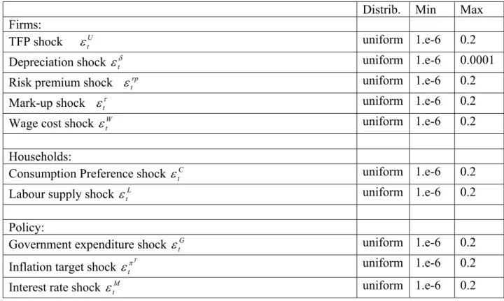
Structural shocks. After in initially setting priors to inv-gamma, the traditional priors of standard errors in Bayesian analysis, we preferred to set up flat priors in a relatively large interval of values, reflecting more clearly our prior ‘ignorance’ about possible values of shocks. Above all in view of a complete Bayesian comparison with other models (VARs), this assumption might be revisited by considering, e.g., a training set. This because too large a prior range might unduly penalise the present model, by giving too low weight to the likelihood (a totally uninformative prior in the range [-inf, inf] would give a uniformly zero weight to any likelihood value, implying the rejection of any model; see Sims, 2003, for a full discussion on these matters).

Concerning the shock to time-varying δ ( ), we set a much smaller range, since we do not want δ to absorb whatever is missed by the rest of the model, but we just allow the minimum shock necessary to reconstruct the depreciation path.

δ ε_t

Table 1.a Priors structural shocks

Distrib. Min Max

Firms: TFP shock U

t

ε uniform 1.e-6 0.2

Depreciation shock ε_tδ uniform 1.e-6 0.0001

Risk premium shock rp

t

ε uniform 1.e-6 0.2

Mark-up shock ετ_t uniform 1.e-6 0.2

Wage cost shock W t

ε uniform 1.e-6 0.2

Households: Consumption Preference shock C

t

ε uniform 1.e-6 0.2

Labour supply shock L

t

ε uniform 1.e-6 0.2

Policy: Government expenditure shock G

t

ε uniform 1.e-6 0.2

Inflation target shock ε_tπT uniform 1.e-6 0.2

Interest rate shock M

t

Table 1.b Priors shock persistence

Parameter Distribution Mean St. dev. Support

Firms:

TFP _ρU _{beta 0.9 0.04 [0 1]}

Depreciation ρδ beta 0.9 0.04 [0 1]

Risk premium _ρrp _{beta 0.5 0.2 [0 1]}

Wage costs _ρW _{beta 0.5 0.2 [0 1]}

Households:

Labour supply _ρL _{beta 0.5 0.2 [0 1]}

Policy:

Government expenditure _ρG _{beta 0.9 0.04 [0 1]}

Inflation target ρπT beta 0.5 0.2 [0 1]

Model parameters.

The model parameters to be estimated have a structural economic interpretation and are therefore restricted to lie in certain intervals dictated by economic theory or implied by long run constraints. The following ranges have been chosen for the individual coefficients:

Table 2 Priors model parameters

Parameter Distribution Mean St. dev. Support

Firms:

Depreciation rate δ beta 0.015 0.005 [0 0.2] Capacity utilisation a₂ beta 0.05 0.028 [0 0.1] Adjustment cost, capital γ_K beta 15 5 [0 30] Adjustment cost, inv. γ_I beta 10 3 [0 20]

Adjustment cost, labour γ_L beta 15 5 [0 30]

Adjustment cost, price γ_P beta 15 5 [0 30]

Adjustment cost, wage γ_W beta 15 5 [0 30]

Mark-up, cyclical τ₁ beta -0.1 0.03 [-0.2 0] Share of fwd looking price setters sfp beta 0.6 0.05 [0.5 1]

Households: Habit persistence hab beta 0.6 0.15 [0 0.9] Labour supply elast. κ gamma 0.5 0.4 [0 Inf]

Labour supply const ω gamma 0.2 0.15 [0 Inf] Bargaining strength bg beta 0.375 0.18 [0 0.75]

Wage mark-up θ gamma 2 0.8 [1 Inf]

Policy: Fiscal response to ygap tY

G beta 0 0.4 [-1 1]

Interest rate smoothing ilag beta 0.8 0.1 [0 1]

Interest rate response, t_M∆π beta 0.2 0.09 [0 0.4] Interest rate response, Y

M

t∆ _{beta 0.1 0.045 [0 0.2]}

Interest rate response, t_Mπ beta 1.25 0.3 [0.5 2] Interest rate response, Y

M

t beta 0.3 0.06 [0 0.5]

Smoothness, trend GDP ρ_YPOT beta 0.9 0.05 [0.7 1]

Note: The following parameters were fixed: output elasticity of labour α = 0.5940, discount factor β = 0.989, interest elasticity money demand ζ= -0.4 , Mark-up level τ₀= 0.1;

The remaining parameters are determined by steady state constraints. )

1 )(

(

1= rss+rp+δ γIδ+

a 1st parameter of capacity utilisation

α α − = 1 ss ssK L A Technology constant. ss I ss P I r r =(1−τ)(1−α)δ/ /(γ δ +1)−δ − Risk premium.

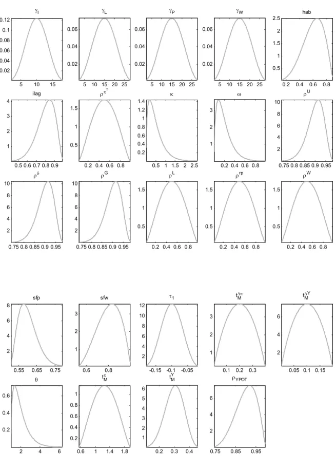
We identified beta or gamma prior distributions for model parameters3_{. The prior} specification of sfp and t required a particular attention, whereby we had to give lower weight to values that were “preferred” by the likelihood, but that implied unreasonable dynamical behaviour in the impulse responses. So, we set asymmetric distributions that privileged the lower part of range for sfp and higher part for t . This implied only a slightly worse fit, but a much better model behaviour in terms of theoretical considerations. This kind of approach is legitimate in a Bayesian framework, and distinguishes from a plain constrained optimisation, which would be considered much more arbitrary. The fact that we give a smaller (but non-zero!) prior probability to some portion of the parameter ranges, always gives the possibility to the likelihood to override this assumption, if the data strongly supports hypotheses about such values that were unlikely a priori. Moreover, this approach does not rule out possible misspecification or the rejection of the present model with respect to competing ones. In the latter case, the integrated likelihood of the present model would be penalised with respect to a competing one that provided more “agreement” between prior assumptions and likelihood shape.

Y M

Y M

The plots of the prior distributions are given below. The model was estimated using the following eight series as observations: Y, I, C, K, L, π, W _P, inom.

3 _{Please note that the support of beta distributions might be larger than the ranges specified in Section 1, but}

means and the standard deviations are set in such a manner that prior probability is larger than zero only in the acceptable range.

Figure 1 Prior distributions 0.05 0.1 0.15 4.5 5 5.5 6 σ(εC_t)

2.e-5 6.e-5 10.e-5 1.e4 σ(εδ_t) 0.05 0.1 0.15 4.5 5 5.5 6 σ(ετ_t) 0.05 0.1 0.15 4.5 5 5.5 6 σ(εG_t) 0.05 0.1 0.15 4.5 5 5.5 6 σ(επ_tT) 0.05 0.1 0.15 4.5 5 5.5 6 σ(εL t) 0.05 0.1 0.15 4.5 5 5.5 6 σ(εM t) 0.05 0.1 0.15 4.5 5 5.5 6 σ(εU t) 0.05 0.1 0.15 4.5 5 5.5 6 σ(εrp t ) 0.05 0.1 0.15 4.5 5 5.5 6 σ(εW t ) 0.03 0.06 0.09 7 8 9 10 a₂ 0.2 0.4 0.6 0.5 1 1.5 barg 0.01 0.02 0.03 20 40 60 80 δ -0.5 0 0.5 0.2 0.4 0.6 0.8 tY_G 5 10 15 20 25 0.02 0.04 0.06 γ_K

Figure 1 (cont’d) Prior distributions 5 10 15 0.02 0.04 0.06 0.08 0.1 0.12 γ_I 5 10 15 20 25 0.02 0.04 0.06 γ_L 5 10 15 20 25 0.02 0.04 0.06 γ_P 5 10 15 20 25 0.02 0.04 0.06 γ_W 0.2 0.4 0.6 0.8 0.5 1 1.5 2 2.5 hab 0.5 0.6 0.7 0.8 0.9 1 2 3 4 ilag 0.2 0.4 0.6 0.8 0.5 1 1.5 ρπT 0.5 1 1.5 2 2.5 0.2 0.4 0.6 0.8 1 1.2 1.4 κ 0.2 0.4 0.6 0.8 1 2 3 ω 0.75 0.8 0.85 0.9 0.95 2 4 6 8 10 ρU 0.75 0.8 0.85 0.9 0.95 2 4 6 8 10 ρδ 0.75 0.8 0.85 0.9 0.95 2 4 6 8 10 ρG 0.2 0.4 0.6 0.8 0.5 1 1.5 ρL 0.2 0.4 0.6 0.8 0.5 1 1.5 ρrp 0.2 0.4 0.6 0.8 0.5 1 1.5 ρW 0.55 0.65 0.75 2 4 6 8 sfp 0.6 0.8 1 2 3 sfw -0.15 -0.1 -0.05 2 4 6 8 10 12 τ₁ 0.1 0.2 0.3 1 2 3 t∆π_M 0.05 0.1 0.15 2 4 6 t∆_MY 2 4 6 0.2 0.4 0.6 θ 0.6 1 1.4 1.8 0.2 0.4 0.6 0.8 1 tπ_M 0.2 0.3 0.4 1 2 3 4 5 6 tY_M 0.75 0.85 0.95 2 4 6 ρ_YPOT

4.2 Parameter estimates and shocks identified

The posterior estimation followed the methodology of Section 2. First the mode of the posterior is estimated using a non-linear optimisation routine (values reported in the Annex).

Then, a sample from the posterior distribution is obtained with the Metropolis algorithm using the inverse Hessian at the posterior mode as the covariance matrix of the jumping distribution. The scale coefficient was set to 0.25, allowing a good acceptation rate (25%). We ran 4 parallel Markov chains. Since the refinement of the convergence tests proceeded slowly by increasing the length of the chains, we decided to update the covariance matrix of the jumping distribution according to the last portion (30%) of the chains based on the inverse Hessian. This allowed us to obtain good convergence tests of 4 new chains (of 40,000 runs each) based on the updated covariance matrix.

Figure 2 Convergence test Metropolis MCMC

0 0.5 1 1.5 2 2.5 3 3.5 4 x 104 100 101 102 Multivariate PSRF 0 0.5 1 1.5 2 2.5 3 3.5 4 x 104 10-180 10-160 10-140 det(Σ) within chain between chain

This Figure shows the convergence tests for Metropolis MCMC. Upper panel shows the multivariate potential scale reduction factor, which should be near to 1 at convergence. Lower panel shows the determinant of the ‘between chains’ and ‘within chains’ covariance matrices of the Monte Carlo sample.

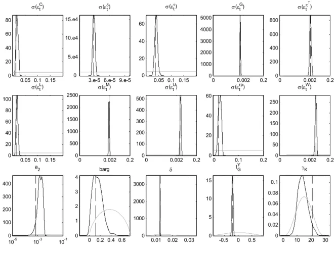
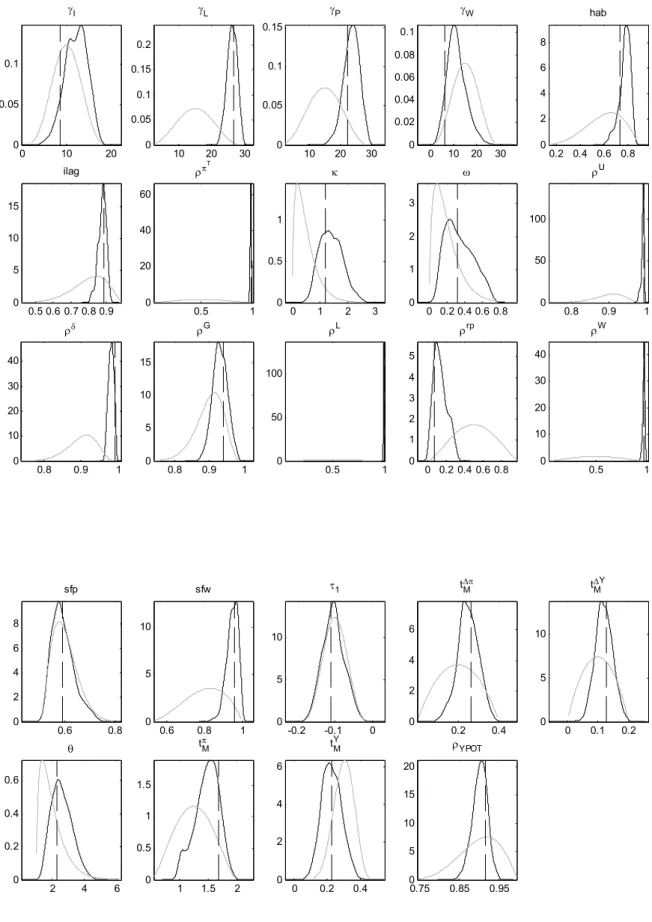
After discarding the initial 70% of runs, we could proceed to the Bayesian inference. The following figures show the estimated marginal posterior distributions (black lines), compared to priors (grey lines) and the point estimate of the multivariate mode (vertical dashed lines). It is interesting to note that for some parameters the maximum of the marginal distribution is shifted with respect to the mode of the multivariate distribution (in particular γ_K and γ_I ). This implies that such a local maximum is in a very narrow region with almost zero mass, related to very specific parameter combinations. To give an idea of this, it is interesting to

note that the log-posterior at the mode is about 3800, while the Markov chains evolve in a range [3760 – 3792] i.e. almost 10 log-points lower with respect to the mode. In spite of this quite high difference in level, even imposing a starting point very near to the mode, the evolution of the Markov chain evolved similarly to the ones shown here, implying that such a local optimum is located in a region so small to imply an almost zero probability for a chain to fall there. In the Annex we also report the values of the posterior mean with confidence bands for the estimated parameters. The logarithm of the marginal likelihood for this model is about 3663.

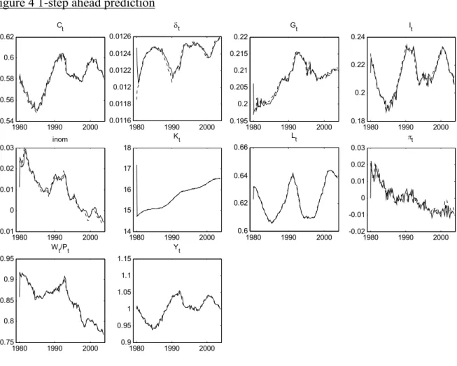
Finally, Figure 4 shows the 1-period ahead predictions of the model for the main model variables, including the depreciation rate δ and government expenditure G. Dashed lines are observations; continuous lines are model predictions. On the whole, the model fits the data remarkably well. One point that is particularly noteworthy is that the model over-predicts inom in the last years (coupled with loose M).

t

ε

Figure 3 Prior and posterior distributions standard errors structural shocks and parameters

0.05 0.1 0.15 0 20 40 60 80 σ(εC t)

3.e-5 6.e-5 9.e-5 0 5.e4 10.e4 15.e4 σ(εδ t) 0.05 0.1 0.15 0 20 40 60 σ(ετ t) 0 0.002 0.2 0 1000 2000 3000 4000 5000 σ(εG t) 0 0.002 0.2 0 200 400 600 800 σ(επT t ) 0.05 0.1 0.15 0 20 40 60 80 100 σ(εL_t) 0 0.002 0.2 0 500 1000 1500 2000 2500 σ(εM_t) 0 0.002 0.2 0 100 200 300 400 500 σ(εU_t) 0 0.1 0.2 0 20 40 60 σ(εrp_t ) 0 0.002 0.2 0 50 100 150 200 250 σ(εW_t ) 10-5 10-3 10-1 0 100 200 300 400 a₂ 0 0.2 0.4 0.6 0 1 2 3 4 barg 0.01 0.02 0.03 0 1000 2000 3000 δ -0.5 0 0.5 0 5 10 15 tY_G 0 10 20 30 0 0.02 0.04 0.06 0.08 0.1 γ_K

Figure 3(cont’d) Prior and posterior distributions standard errors structural shocks and parameters 0 10 20 0 0.05 0.1 γ_I 10 20 30 0 0.05 0.1 0.15 0.2 γ_L 10 20 30 0 0.05 0.1 0.15 γ_P 0 10 20 30 0 0.02 0.04 0.06 0.08 0.1 γ_W 0.2 0.4 0.6 0.8 0 2 4 6 8 hab 0.5 0.6 0.7 0.8 0.9 0 5 10 15 ilag 0.5 1 0 20 40 60 ρπT 0 1 2 3 0 0.5 1 κ 0 0.2 0.4 0.6 0.8 0 1 2 3 ω 0.8 0.9 1 0 50 100 ρU 0.8 0.9 1 0 10 20 30 40 ρδ 0.8 0.9 1 0 5 10 15 ρG 0.5 1 0 50 100 ρL 0 0.2 0.4 0.6 0.8 0 1 2 3 4 5 ρrp 0.5 1 0 10 20 30 40 ρW 0.6 0.8 0 2 4 6 8 sfp 0.6 0.8 1 0 5 10 sfw -0.2 -0.1 0 0 5 10 τ₁ 0.2 0.4 0 2 4 6 t∆π_M 0 0.1 0.2 0 5 10 t∆_MY 2 4 6 0 0.2 0.4 0.6 θ 1 1.5 2 0 0.5 1 1.5 tπ_M 0 0.2 0.4 0 2 4 6 tY_M 0.75 0.85 0.95 0 5 10 15 20 ρ_YPOT

Figure 4 1-step ahead prediction 1980 1990 2000 0.54 0.56 0.58 0.6 0.62 C_t 1980 1990 2000 0.0116 0.0118 0.012 0.0122 0.0124 0.0126 δ_t 1980 1990 2000 0.195 0.2 0.205 0.21 0.215 0.22 G_t 1980 1990 2000 0.18 0.2 0.22 0.24 I_t 1980 1990 2000 -0.01 0 0.01 0.02 0.03 inom 1980 1990 2000 14 15 16 17 18 K_t 1980 1990 2000 0.6 0.62 0.64 0.66 L_t 1980 1990 2000 -0.02 -0.01 0 0.01 0.02 0.03 π_t 1980 1990 2000 0.75 0.8 0.85 0.9 0.95 W_t/P_t 1980 1990 2000 0.9 0.95 1 1.05 1.1 1.15 Y_t 4.3 VAR comparison

If we compare the RMSE’s of the DSGE model computed at the posterior mean, with the RMSE’s of a VAR(1) model with the same 8 observed series : Y, I, C, K, L, π, W _P, inom. Table 3 RMSE comparison with VAR

RMSE's VAR model (post. mean) C 5.9398e-006 8.5811e-006

I 5.5508e-006 8.388e-006 inom 1.4206e-006 2.2686e-006 K 0.00037479 1.0741e-005 L 5.2953e-007 6.7359e-007

π 4.5673e-006 9.9136e-006 W/P 1.9294e-005 2.3478e-005 Y 1.9422e-005 2.6547e-005

RMSE’s of the DSGE are higher but of the same order of magnitude than the VAR, except for K, where the VAR performs much worse (RMSE is forty times larger).

5 Which structural shocks drive the euro economy?

One of the major advantages of the modelling approach used here is that system estimation of the model yields, besides the posterior distribution of the model parameters, structural shocks which have an unambiguous interpretation and which can help us understand the current economic situation. The structural shocks identified in the estimation of this model are shocks to households, firms, government and fiscal policy. Households are affected by shocks to preferences for consumption and labour supply. Firms are hit by shocks to technology, mark-ups, adjustment costs for labour and capital and a risk premium shock.

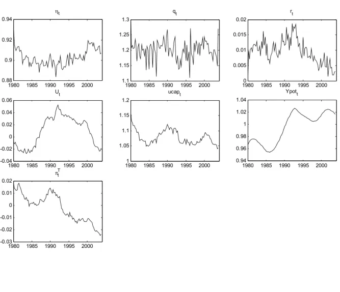
Several aspects of the estimated shocks (figure 5) and implied unobserved variables (figure 6) are worth highlighting.

Demand Shocks

The consumption preference shock appears slightly negative at the end of the estimation sample. This suggests lower preferences for consumers spending and may be a reflection of savings uncertainty concerning future pensions and tax liabilities. Notice, however, the size of the shock is not extraordinary large, given the fluctuations of over the entire sample period. Investment is hit by two autonomous shocks, a risk premium shock and a shock to adjustment costs. The latter are unimportant and not further considered. The risk premium shock ( ) does not show any particular trend and appears to behave normally in recent years. This suggests that investment fluctuations are explained by fundamentals. The smoothed auto-correlated fiscal policy shock z( ) displays a turnaround in 2000-01. The fall in this auto-correlated shock shows clearly the fiscal consolidation period starting in the late 1980s, but the declining trend in government spending is reversed in the early 2000s. This refutes the view that fiscal policy has been overly restrained by the SGP and been less countercyclical over the last years.

C t ε C t ε rp t ε G t ε Supply shock

Our Kalman filter estimation allows to decompose observed total factor productivity into a capacity utilisation and a ‘true TFP’ component (denoted as U). According to these estimates U shows a trend increase in the second half of the 1980s, a movement along the trend in the 90s, but a sharp decline in the late 1990s- early 2000s. Thus the fall in TFP in the recent past is largely a structural phenomenon and not the result of a lack in demand, since capacity utilisation (UCAP) shows a normal cyclical behaviour in recent years. Notice, TFP is also one of the major driving forces of investment and is therefore one of the fundamental factors for the slowdown of investment. Trends and fluctuations in mark-ups are important measures for the supply potential of the euro area economy. According to these estimates the mark-up has declined on average since the early 1990s (η=1-mark-up) from around 10 to 8%. This could reflect increased competitive pressure due to goods market reforms (internal market programme) but also increased pressure from global competition.

Labour market shocks

The model identifies a labour supply ( ) and a labour demand shock ( ). The trend increase in labour supply (or in model terms a trend decline in the preference for leisure (Z( )) after 1995 is consistent with the observation of increased labour force participation and a declining NAIRU in the Euro area. Notice, however, the shock to labour supply has a pronounced cyclical pattern, which suggests that the simple wage rule used here does not

L t ε W t ε L t ε

properly account for the dynamic adjustment of wages over the business cycle. On the other hand, the upward trend of Z( ) reflects the increase in non-wage labour costs over the sample. Interestingly this trend has stopped in the late 1990s, possibly reflecting a success of various labour market reform measures intended to reduce regulatory burdens for firms related to employment. W t ε M t 85 19 0-4 1985 19 1985 19

Monetary policy shocks

The monetary policy shock is negative for the years after 2000. This would suggest a looser monetary stance than suggested by the estimated Taylor rule. This could be linked to an underestimation of the decline in the inflation objective π

ε

T_{, which shows a clear trend decline,} but may nevertheless underestimate the actual decline in the monetary policy’s inflation objective. This is one aspect that may need further attention in future extensions of this model. Figure 5 Estimated smoothed shocks at the posterior mean

1985 1990 1995 2000 -0.05 0 0.05 εC_t 19 90 1995 2000 -1 0 1x 1 εδ t 1985 1990 1995 2000 -0.1 -0.05 0 0.05 0.1 ετ t 1985 1990 1995 2000 -5 0 5 10x 10 -3 z(εG_t) 1985 1990 1995 2000 -6 -4 -2 0 2 4x 10 -3 επT t 90 1995 2000 -0.2 -0.1 0 0.1 0.2 z(εL t) 1985 1990 1995 2000 -4 -2 0 2 4 6x 10 -3 _εM t 1985 1990 1995 2000 -0.01 -0.005 0 0.005 0.01 0.015 εU_t 1985 1990 1995 2000 -0.1 -0.05 0 0.05 0.1 z(εrp_t ) 90 1995 2000 -0.1 -0.05 0 0.05 0.1 z(εW_t )

Figure 6 Unobserved variables 1980 1985 1990 1995 2000 0.88 0.9 0.92 0.94 η_t 1980 1985 1990 1995 2000 1.1 1.15 1.2 1.25 1.3 q_t 19800 1985 1990 1995 2000 0.005 0.01 0.015 0.02 r_t 1980 1985 1990 1995 2000 -0.04 -0.02 0 0.02 0.04 0.06 U_t 19801 1985 1990 1995 2000 1.05 1.1 1.15 1.2 ucap_t 1980 1985 1990 1995 2000 0.94 0.96 0.98 1 1.02 1.04 Ypot_t 1980 1985 1990 1995 2000 -0.03 -0.02 -0.01 0 0.01 0.02 πT_t

6 Estimated impulse responses of structural shocks

In this section, we present the estimated impulse responses of the nine structural shocks in our model. The impulse response are generated on the basis of the reduced form representation of the model (policy and reaction functions - see annex). This is particularly simple, since the reduced form is a linear model (formally equivalent to a multivariate ARMA). They depict the responses for the endogenous variable following a one-period shock to each of the structural shocks (which are in most cases auto-correlated), each for a 5 year (20 periods) horizon. A full Bayesian IRF analysis is here presented, picking 1,000 samples out of the full Monte Carlo sample and computing IRF’s for each of them. Finally, the mean path (solid lines) and the confidence band (dashed lines) can be obtained, as shown in the Figures.

Figure 7 Consumption preference shock C t ε 0 10 20 -0.02 0 0.02 0.04 0.06 Y(%) vs εC 0 10 20 -0.04 -0.03 -0.02 -0.01 0 I(%) vs ε C 0 10 20 -0.02 0 0.02 0.04 0.06 0.08 C(%) vs ε C 0 10 20 -4 -3 -2 -1 0x 10 -3 _{K(%) vs ε}C 0 10 20 -5 0 5 10x 10 -3 _{L(%) vs ε}C 0 10 20 -0.01 0 0.01 0.02 0.03 0.04 M/P(%) vs ε C 0 10 20 -2 0 2 4 6 8x 10 -5 _{π vs ε}C 0 10 20 -10 -5 0 5x 10 -3 _{W/P(%) vs ε}C 0 10 20 -0.2 0 0.2 0.4 0.6 0.8 inom(%) vs ε C

Figure 7 presents the estimated effect of a consumption preference shock ( ). This shock is a combined shock affecting consumption and leisure choice and has a direct impact on consumption and labour supply (through λ). The effect of this preference shock is to raise consumption by 0.06 percent, and employment by 0.007 per cent (in the second period after the shock). The boost to demand raises inflation and nominal interest rates rise, but the presence of adjustment costs limits the extent of the price rise. The shock leads to crowding out of investment and a decumulation of capital.

C t

Figure 8 Shock to depreciation rate (ε_tδ) 0 10 20 -0.06 -0.04 -0.02 0 0.02 Y(%) vs ε δ 0 10 20 -0.5 -0.4 -0.3 -0.2 -0.1 0 I(%) vs ε δ 0 10 20 0 0.05 0.1 0.15 0.2 C(%) vs ε δ 0 10 20 -0.2 -0.15 -0.1 -0.05 0 K(%) vs ε δ 0 10 20 -0.05 -0.04 -0.03 -0.02 -0.01 0 L(%) vs ε δ 0 10 20 -0.06 -0.04 -0.02 0 0.02 M/P(%) vs ε δ 0 10 20 -2 0 2x 10 -4 _{π vs ε}δ 0 10 20 -0.02 0 0.02 0.04 0.06 W/P(%) vs ε δ 0 10 20 -1.5 -1 -0.5 0 0.5 1 inom(%) vs ε δ 0 10 20 0.1 0.15 0.2 0.25 0.3 0.35 δ(%) vs ε δ

Figure 8 depicts a shock to the depreciation rate of 0.25 per cent on impact. This implies an increase in the cost of capital of 0.012 percentage points. This shock is highly persistent, in fact is has not disappeared after 100 periods, due to the large estimated autocorrelation term in the depreciation rate. The increase in the cost of capital leads to a decline in investment and the capital stock, lower real rates, higher consumption, higher real wages and lower employment. Note however, the large confidence bands, which suggest a large margin of uncertainty surrounding this type of shock.