Optimal monetary policy rules for the euro area: an analysis using the area wide model

(1)

W O R K I N G PA P E R S E R I E S

N O. 3 6 0 / M AY 2 0 0 4

OPTIMAL

MONETARY POLICY

RULES FOR THE

EURO AREA: AN

ANALYSIS USING

THE AREA WIDE

MODEL

(2)

In 2004 all publications will carry a motif taken from the €100 banknote.

W O R K I N G PA P E R S E R I E S

N O. 3 6 0 / M AY 2 0 0 4

OPTIMAL

MONETARY POLICY

RULES FOR THE

EURO AREA: AN

ANALYSIS USING

THE AREA WIDE

MODEL

1

by Alistair Dieppe

2

_{, Keith Küster}

3

and Peter McAdam

2

This paper can be downloaded without charge from http://www.ecb.int or from the Social Science Research Network electronic library at http://ssrn.com/abstract_id=533105.

(3)

© European Central Bank, 2004 Address

Kaiserstrasse 29

60311 Frankfurt am Main, Germany Postal address

Postfach 16 03 19

Reproduction for educational and non-commercial purposes is permitted provided that the source is acknowledged. The views expressed in this paper do not necessarily reflect those of the European Central Bank.

The statement of purpose for the ECB Working Paper Series is available from the

(4)

C O N T E N T S

Abstract 4

Non-technical summary 5

1 Introduction 6

2 The modelling framework 8

3 The area wide model 11

3.1 Evaluation of estimated policy rules 13

3.2 The Taylor principle – determinacy

regions 17

4 Optimal policy 19

4.1 Optimized simple rules vs. optimal

discretionary policy 20

4.2 Benchmarking against commitment 30

5 Optimal forecast horizons 33

5.1 Optimal forecast horizons for inflation 33

5.2 Optimal forecast horizons for both

the output gap and the inflation rate 37

6 Conclusions 38

References 40

A Linearization and parameter choices 43

B First-order form 45

C Empirical variance covariance matrix

and data 45

D Calculation of optimal policy 46

E Upper bound on ␴_⌬_rfor discretion 46

F Optimal commitment 47

G Sensitivity analysis of results 47

(5)

Abstract

In this paper, we analyze optimal monetary policy rules in a model of the euro area, namely the ECB’s Area Wide Model, which embodies a high de-gree of intrinsic persistence and a limited role for forward-looking expecta-tions. These features allow us, in large measure, to differentiate our results from many of those prevailing in New Keynesian paradigm models. Specifi-cally, our exercises involve analyzing the performance of various generalized Taylor rules both from the literature and optimized to the reference model. Given the features of our modelling framework, we find that optimal policy smoothing need only be relatively mild. Furthermore, there is substantial gain from implementing forecast-based as opposed to outcome-based policies with the optimal forecast horizon for inflation ranging between two and three years. Benchmarking against fully optimal policies, we further highlight that the gain of additional states in the rule may compensate for a reduction of communicability. Thus, the paper contributes to the debate on optimal mon-etary policy in the euro area, as well as to the conduct of monmon-etary policy in face of substantial persistence in the transmission mechanism.

JEL: E4, E5

(6)

Non-technical summary

In this paper, we examine optimal monetary policy in a medium-sized model of the euro area, namely the Area Wide Model (AWM), Fagan et al. (2001). The choice of model is interesting for a number of reasons. First, it contributes to the debate about optimal monetary policy rules for the new euro area; this is a relatively underdeveloped area of research so far. Second, the AWM makes some notable departures from the class of models conventionally studied in the optimal monetary policy literature.

These AWM model features - namely, a high degree of intrinsic persistence and a limited role for forward-looking expectations - allow us, in large measure, to diﬀerentiate our results from many of those prevailing in “New-Keynesian” paradigm models (which tend to be highly forward-looking and “micro-founded”).

Specifically, our exercises involve analyzing the performance of various generalized Tay-lor rules both from the literature and optimized to the reference model. Given the features of our modelling framework, we find that optimal policy “smoothing” (i.e. the degree of policy gradualism) need only be relatively mild. Furthermore, there is substantial gain from implementing forecast-based (i.e., forward-looking) as opposed to outcome-based policies (i.e., backward or contemporaneous horizons) with the optimal forecast horizon for inflation ranging between two and three years. Benchmarking simple optimal rules against fully optimal policies, we further highlight that the gain of additional targets in the rule may compensate for a reduction of communicability. That is to say, more com-plicated rules may significantly outperform relatively simple (and easy to communicate) ones like the Taylor rule.

(7)

1 Introduction

In stochastic macro-economic environments subject to nominal rigidities, monetary policy can actively contribute to stabilizing the real and nominal economy. Accordingly, a large body of work has evolved around examining optimal monetary policy rules in sticky-price models. These may be backward-looking as in Svensson (1997) and Ball (1999) or small micro-founded forward-looking models (for early references, Clarida et al., 1999). Such models tend to imply that optimal policy can be written as (or closely approximated by) a Taylor (1993) rule. Often such models feature only a small number of states; consequently, there is only a minor loss in stabilization by limiting feedback to only a subset of such states.

Policy implications for larger scale models, however, have received somewhat less at-tention – being largely focused on models which assume that agents are substantially forward-looking, as in Levin et al. (1999, 2003). Notwithstanding, the degree to which expectations are in fact forward looking is far from being settled on empirical grounds (e.g., Fuhrer and Estrella, 2002, Fuhrer 1997). In the light of model uncertainty, a pru-dent policy-maker may therefore feel startled by the strong emphasis on forward-looking expectations combined with small-scale models and in solving this may be unwilling to only resort to small-scale backward-looking models for policy advice.

In this paper, we therefore examine optimal monetary policy in a medium-sized model of the euro area, namely the Area Wide Model (AWM), Fagan et al. (2001). The choice of model is interesting for a number of reasons. First, it contributes to the debate about optimal monetary policy rules for the new euro area; this is a relatively underdeveloped area and therefore of high value added.1 _{Second, the AWM makes some notable}

depar-tures from the class of models conventionally studied in the optimal monetary policy literature – these include a signiﬁcant deviation from the strong forward-lookingness and low persistence emphasized in the recent literature as well as from the compact dynamics and limited state variables found in such models. For such reasons, the AWM may be a good candidate for deriving policy implications and benchmarking those against others in the literature.

Deﬁning policy makers’ preferences as a weighted average of inﬂation and output

sta-1_{The model, for instance, is used extensively in simulation and projection analysis at the ECB. See for}

(8)

bilization (conditioning on instrument stability), we examine the performance of simple optimized monetary policy rules and fully optimal policy against estimated Taylor rules. In doing so, we also assess the optimal forecast horizon in such monetary policy rules and highlight sources for possible indeterminacy. A key feature of our results is the importance played by intrinsic persistence (i.e., persistence not introduced by monetary policy itself). Coenen (2002), for example, emphasized the risks of underestimating inflation persistence in deriving policy rules. The AWM in fact incorporates substantial intrinsic persistence alongside a sufficiently rich structure and largely backward-looking expectations. Such model differences – from, say, a standard “New-Keynesian” paradigm model – may po-tentially serve as a robustness check. In particular, we find that – in contrast to many studies, e.g., Levin et al. (2003) – substantial smoothing of interest rates in addition to that induced by persistence of feedback variables is not necessarily a feature of optimal monetary policy. Similarly, given the size of our model we find that the simple optimal rules need not necessarily approximate fully optimal ones (see also, Finan and Tetlow, 1999). Finally, we find that optimal inflation (and output gap) forecast horizons are larger than typically found in the literature owing to the sizeable inflation persistence and the limited degree of forward-lookingness in the model.

Taking these results literally and abstracting from model and policy uncertainty2_{, our}

analysis suggests that optimal policy should be focused on future states of the economy and incorporate a broad set of information even at the risk of loosing the communicability of policy rules. Indeed, gains from fully optimal discretionary and commitment policy are sizeable due to the persistence of the economy.

The paper proceeds as follows. Section 2 introduces the modelling framework. Section 3 oﬀers a description of the key features of the AWM before section 4 analyzes their implications for the performance of simple optimal rules relative to optimal discretionary policy and more complicated commitment rules. A further section considers the question of the optimal forecast horizon. Section 6 concludes with some policy advice and some considerations of the implications of model uncertainty for the results derived.

2_{It should be borne in mind that policy rules of the kind we discuss are to be regarded as broad}

approximations to actual policy decisions and trade oﬀs. For instance, other than model and parameter uncertainty as mentioned above, we assume rational expectations on behalf of both the central bank and the private sector. Among other things, this amounts to the assumption that the private sector forecast model coincides with the AWM. Another caveat includes the availability of reliable real-time data (e.g., Orphanides, 2001).

(9)

2 The Modelling Framework

The AWM is not derived explicitly from micro-foundations. We therefore follow the literature in modelling the preferences of a central bank by a conventional quadratic loss function deﬁned in terms of unconditional variances of inﬂation and the output gap,3

L= min

r {V(π) +λV(gap) +γV(∆r)}, (1)

where V(·) marks the unconditional variance of annual(ized) inﬂation (π), the output gap (gap) and interest rate changes (∆r), respectively.4 _{While the policymaker’s prime}

mandate is to keep inflation low and stable around a target, he may also have a mandate for stabilizing output around its potential,5 _{the case of flexible inflation targeting in the}

wording of Svensson (1999). The relative weight of these conﬂicting goals in the presence of cost-push shocks is captured by the preference parameter λ∈R₊.6

A typical ﬁnding in model-based optimization exercises is that movements in the policy instrument exceed that witnessed in the data. Indeed, as we earlier discussed some degree of policy smoothing is an established empirical regularity. For instance, central banks may be reluctant to change short-term rates frequently in so far as it undermines credibility and inhibits ﬁnancial-market stability – Cukierman (1990) provides a survey on interest-rate smoothing. Uncertainty provides another rationale. Policymakers may be unwilling to completely rely on (model) certainty equivalent policy for pursuing stabilization in the presence of uncertainty about the transmission mechanism, as in Brainard (1967). To capture such features, Svensson (1999) implements a weight, γ > 0, on changes of interest rates directly in the loss-function. Additionally, to derive implications directly linked to the current euro area policy environment, we impose an upper bound on interest

3_{Subsequently, all variables will be in deviations from steady-state values.}

4_{Rotemberg and Woodford (1998) and others have shown that similar loss functions can be derived as}

a second-order approximation to a representative agent’s utility function in a simple New-Keynesian model.

5_{Note that here there is no inﬂation bias.}

6_{In a stationary model like ours, this preference function is the limiting case as the policymaker stops}

discounting of the more standard loss function in curly brackets

L= lim β→1(1−β)   minr E ∞ j=0 βj_π2 j +λgap2j+γ(∆rj)2   .

(10)

rate variability of the empirical size while setting γ = 0.7 As an added beneﬁt, such a constraint precludes zero-bound solutions for the nominal rate.

Svensson (1999a) argues that central banks should follow target rules, assuring the public to enact policy such that it brings internal inflation and possibly output gap fore-casts on track with the target(s) in a horizon depending on policy lags. The form of these targeting rules that is communicated to the public is potentially robust to param-eter changes since forecasts themselves incorporate all new information.8 However, such a strategy may imply rather complex feedback rules, since in principle they would incor-porate all the (predetermined) states of the model. Nonetheless, in some cases they may be concisely rewritten in terms of expectations of future inflation and/or the output gap. In general, however, being more complicated, such an instrument rule may be hard to communicate to, and be monitored by, the public. In our view, Svensson’s framework might be best described as implementing optimal policy under discretion – we use this as a natural benchmark. Other authors, like Batini and Haldane (1999), understand infla-tion targeting directly in terms of a simple instrument rule, the most prominent of which may be Taylor’s (1993) rule, a generalized version of which is

rt=ρrt−1+αEtπt+θ+βEtgapt+κ, (2)

where ρ ≥ 0 represents the degree of policy smoothing,9 expectations are rational, and (α, β)∈R2

+,with the forecast horizons (θ, κ)∈Z2.10

From an institutional viewpoint, the advantage of simple rules is their transparency

7_{We also experimented with a larger upper bound of 2.5 times the empirical upper bound and with}

implementing a weight on changes of interest rates directly in the loss function. As one could expect, with interest changes being less costly, there is somewhat less smoothing of interest rates and a better stabilization performance. Overall, however, the qualitative results remain unchanged.

8_{Nevertheless, changes in the forecasting model of the central bank or parameter uncertainty will}

inevitably change the way forecasts respond to state variables and thereby they will change the feedback rule of the central bank, i.e. the way interest rates are actually set in response to state variables.

9_Typically_ρ _{is estimated at 0.9 for monthly data (}_e.g. _Clarida _{et al.,} _{1998). Often ’policy rules’ are}

taken from models featuring multiple interdependent equations in which case strictly speaking there does not exist an identified “monetary policy equation”. As an example, even under the plain Taylor rule the first order serial correlation coefficient of interest rates isCor₁(r) = 0.95 in the AWM, with

Cor₂(r) = 0.89. Hence, parameterρtakenper se is a poor guide to any assertion about interest rate smoothing as actually observed, but may rather be understood as a guide to practical policy-making.

10_{Approximate and in some cases exact forms of this rule are optimal for a central bank that has a}

quadratic loss function over inﬂation and output – as in (1) – in standard macroeconomic environments (e.g., Svensson, 1999, and Ball, 1999).

(11)

and, thus, the ease with which they may be communicated to and be monitored by the outside world. While it is unlikely that any central bank will follow the literal execution of such a rule, they may nonetheless be a good summary guide to rule based policy in general. Furthermore, simple rules (or the implications thereof) are arguably more robust to model mis-specification and uncertainty (see Levin et al., 1999, Levin and Williams, 2003) than policy based on a larger set of states, which might overfit specific model characteristics.

Furthermore, from an empirical point of view, generalized Taylor rules seem to match the data well for the flexible inflation-targeting periods of central banks in Europe and the US. See, for instance, Clarida et al. (1998, 2000), Gerlach and Schnabel (2000) and Gerdesmeier and Roffia (2003). In some cases other variables may enter significantly into the rules, such as exchange rates (e.g., so-called open-economy monetary policy rules), monetary gaps or financial market indicators. Notwithstanding, a principal advantage of even simple forecast-based rules is that a suitable choice of forecast horizon can incorpo-rate contemporaneous and leading-indicator information and, by effectively accounting for policy-transmission lags, induce successfully pre-emptive policy, while lagged or contem-poraneous rules necessarily operate at or after the event – an aspect Batini and Haldane (1999) call “lag-encompassing”. Second, forecast-based feedback rules are “information-encompassing”: if expectations are rational, they will incorporate all states of the economy and make use of all the structure of the economy (though in a restricted way). By choice of optimal feedback horizons, θ andκ, the central bank can thus considerably govern how information is implemented into even a simple Taylor rule like (2).

Although the generalized Taylor rule seems to be easily implemented, some caveats emerge. For example, there may be lack of reliable real-time data (see Orphanides, 2001). We thus also employ a Taylor rule feeding back on both, lagged output gaps and inﬂation to assess the loss involved. Further, Bernanke and Woodford (1997) highlight that for successful implementation of forecast targeting, there appears to be no substitute for explicit structural modelling of the economy and extensive information gathering by the central bank. They illustrate that directly targeting private sector expectations (say, via surveys) may introduce large ﬂuctuations and nullify the information content of private sector forecasts. The borderline at which the increase in complexity due the information encompassing of forecast based rules hinders monitoring is not easily drawn. At some

(12)

point, a discretionary framework might ﬁt the policy framework better. We therefore report results for stabilization using both forecast-based rules and optimal discretionary policy.

Following the literature, in section 4 we analyze the performance of simple rules as-suming that due to their simplicity, policymakers could credibly commit themselves to such rules indefinitely. We illustrate that there is a substantial deterioration in stabiliza-tion performance involved when contemporaneous data, θ = κ = 0, is not available or reliable, but lagged data, θ = κ = −1, needs to be used to conduct policy. Apart from these outcome-based rules, we illustrate that a common forecast-based rule with a one-year forecast horizon for inflation, θ = 4, κ = 0, yields substantially better stabilization performance, thereby reaffirming the results of Batini and Haldane (1999). While it is commonly found that the commitment value provided by credible Taylor rules outweighs the loss incurred by conditioning policy only on a subset of information, this ranking depends on model characteristics. The greater is the information content of other vari-ables in the economy (besides the output gap, interest rates and inflation) and the less important is the expectations channel (in the extreme, in a backward-looking model, there is no distinction between Discretion and Commitment), the more valuable will be optimal time-consistent policy as opposed to sub-optimal (optimal simple) policy under commitment.

Optimal discretionary policy in the AWM yields substantially better performance than simple rules unless the central bank feeds back on inﬂation expectations roughly two years into the future. When we choose the horizon of forecast-based rules optimally (Section 5) we ﬁnd that these approximate the optimal discretionary stabilization outcome. Due to the more backward-looking structure of the AWM, we demonstrate that if the central bank could tie its hands, conducting relatively complicated rule based commitment policy, it would not do considerably better than under optimal discretionary policy.

3 The Area Wide Model

The Area Wide Model by Fagan et al. (2001) is a quarterly estimated structural macroe-conomic model that treats the euro area as a single economy. It has a long-run classical equilibrium with a vertical Phillips curve but with some short-run frictions in price/wage

(13)

setting and factor demands. Consequently, activity is demand-determined in the short run but supply-determined in the longer run with employment having converged to a level consistent with the exogenously given level of equilibrium unemployment. Stock-ﬂow adjustments are accounted for by, for example, the inclusion of a wealth term in consumption. At present, the treatment of expectations in the model is limited; with the exception of the exchange rate (modelled by forward-looking uncovered interest parity) and the (12-year bond) term structure, the model embodies backward-looking expecta-tions.

The demand channel in the AWM is enacted by short-term interest rates. Long term rates determine government debt payments but do not explicitly enter investment deci-sions. The expectations channel in principle allows monetary policy to influence inflation via wage and price-setting behavior. In addition to these channels, further channels enter through the exchange rate. Apart from an indirect influence of exchange rates on domestic demand, there is also a direct exchange rate channel to consumer price inflation through the price for imported goods.11 _{In the analysis that follows, one of the key variables is}

the output gap. This is defined as the ratio of real GDP to Potential Output, which is defined by an aggregate Cobb-Douglas production function with constant returns to scale and neutral technical progress. For this, the trend total factor productivity has been estimated within-sample by applying the Hodrick-Prescott filter to the Solow Residual derived from the production function.

Full model listing and simulation evidence can be found in Fagan et al. (2001) and Dieppe and Henry (2004). Applications of the model include examining the monetary transmission mechanism (McAdam and Morgan, 2003), real exchange rate determination (Detken et al., 2002), unemployment dynamics (Dieppe et al., 2004) and forecasting strategies (McAdam and Mestre, 2003).

In the absence of shocks, the non-stationary system converges to a balanced growth path, on which price ratios are constant and real GDP components grow at a common rate. Log-linearization of models around their steady state values prior to analysis is

11_{Svensson (2000) argues that the direct exchange rate channel invalidates the use of CPI inﬂation.}

Similarly, such considerations can be considered in line with the debate in Mankiw and Reis (2003), as to which measure of inﬂation (i.e., “core” or headline rate) central banks should use in their monetary policy strategies. Since any contribution towards that debate is outside of the scope of this paper, we restrict ourselves to a consumer price inﬂation measure in order to be comparable to the existing closed economy literature.

(14)

now standard in the literature on optimal and robust policy even for large-scale models (e.g., Levin et al., 1999) and without this step a full-ﬂedged analysis is computationally burdensome.12 _{Appendix A provides details about the linearization.}

In order to shed further light on relevant model properties, we next explore the impli-cations of several estimated rules in the AWM.

3.1 Evaluation of Estimated Policy Rules

The current model version does not incorporate any estimated rule but rather has been calibrated to the standard Taylor one:

rt = 1.5πt+ 0.5gapt. (3)

We also report the properties of incorporating three more rules from the literature into the AWM:

rt= 0.87rt−1+ (1−0.87)(1.93πt+ 0.28gapt), (4)

rt= 0.91rt−1+ (1−0.91)(1.31Etπt+4+ 0.25gapt), (5)

rt= 0.18rt−1+ 1.51Etπt4+4+ 0.28gapt. (6)

Gerdesmeier and Roﬃa (2003) estimate rule (4) on synthetic euro area data from 1985 to 2002. While we do not believe the ECB is a direct successor of the Bundesbank in all respects, we include rule (5), which Clarida et al. (1998) estimate for Germany from 1979 to 1993, as an additional point of reference. Finally, Gerlach and Schnabel (2000) estimate rule (6) for pooled euro area data from 1990 to 1997. This range thus provides two contemporaneous (outcome-based) and two forward-looking (forecast-based) rules.13 Table 1 reports the unconditional standard deviations as implied by the AWM of key variables under these rules.

As can be inferred from the table, the Taylor rule results in large interest changes relative to the data (σ_∆emp_r = 0.569). Some interest-rate smoothing appears therefore to be a necessary feature to match the model to the data. Note that the two rules estimated on synthetic euro data (i.e., rules 4 and 6) ﬁt the historical interest rate volatility quite closely

12_{McAdam and Hughes Hallett (1999) survey linear and non-linear modelling solution algorithms.} 13_{Note that rules (4) and (5) were estimated on monthly data. Accordingly, we adapt those rule to the}

(15)

Table 1: Performance of Given Policy Rulesa Rules σgap σπt σ∆r σr (3) 2.028 1.229 1.530 2.327 (4) 2.406 1.359 0.681 2.444 (5) 2.295 1.390 0.389 1.702 (6) 1.896 1.177 0.626 1.852

a _{For the four diﬀerent generalized Taylor rules the unconditional}

standard deviation of the output gap, of annualized quarterly inﬂa-tion rates, of the annualized interest rate (in percentage terms) and of interest rate changes is reported. The policymaker is assumed to credibly commit to these rules once and forever.

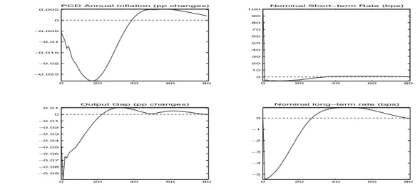
when implemented in the AWM. In light of the stabilization gain comparing forward-looking policy (6) to the other policy rules, we conclude that “good” policy conduct seems to include smoothing and that there appears to be some leeway for monetary policy in inﬂuencing the economy for medium-run stabilization purposes. Supporting this, ﬁgures 1 to 4 report impulse responses to a 100 basis point temporary (1 quarter) rise in short-term nominal interest rates for rules (3) to (6).

0 20 40 60 80 −0.025 −0.02 −0.015 −0.01 −0.005 0 0.005

PCD Annual Inflation (pp changes)

0 20 40 60 80 0 10 20 30 40 50 60 70 80 90 100

Nominal Short−term Rate (bps)

0 20 40 60 80 −0.09 −0.08 −0.07 −0.06 −0.05 −0.04 −0.03 −0.02 −0.01 0 0.01

Output Gap (pp changes)

0 20 40 60 80 −5 −4 −3 −2 −1 0

Nominal long−term rate (bps)

Figure 1: Impulse-responses to a 100bps temporary unanticipated monetary policy shock. The monetary policy rule is the plain Taylor rule (ρ= 0, α = 1.5, β = 0.5). All variables are measured in percentage points deviation from steady state.

(16)

0 20 40 60 80 −0.08 −0.06 −0.04 −0.02 0 0.02

0 20 40 60 80 0 20 40 60 80 100

0 20 40 60 80 −0.15 −0.1 −0.05 0 0.05

0 20 40 60 80 −15 −10 −5 0 5

Figure 2: Impulse-responses to a 100bps temporary unanticipated monetary policy shock. The monetary policy rule is the Gerdesmeier and Roﬃa (2003) rule (4). All variables are measured in percentage points deviation from steady state.

long-lasting effects on output and inflation, with the latter being especially sluggish. In addition, the impulse responses illustrate that a poor conduct of monetary policy could introduce quite pronounced noise at business cycle frequencies. Under the Taylor rule (3), an unanticipated monetary contraction by 100 basis points reduces inflation rates moderately. These reach a trough at a reduction of 0.028 percentage points in inflation more than four years after the shock. Secondary cycles lead to a minor increase in inflation thereafter. The Taylor rule illustrates that while the monetary feedback rule per se does not feature any smoothing, model properties may lead to substantial persistence of shocks. The short-term rate is sharply reduced to a level of 5.98bps below steady-state in the quarter following the shock, from where it returns only slowly to its steady state value, cycling around steady-state at low frequencies. Output in the short-run is far more responsive than the nominal side, reaching its trough of 0.1% below steady state in the quarter following the shock. Again, even in the absence of persistent monetary policy per se, model features introduce secondary cycles with output being 0.01% percent above steady state 8 years after the shock.

Central banks obtain a stronger lever on demand components when committing to more pronounced smoothing. This becomes apparent for the Gerdesmeier and Roﬃa (2003) rule when implemented in the AWM. Here, the real and nominal sides show stronger amplitudes, in addition to peaking later. The maximum reduction of annual inﬂation is three times larger than under a plain Taylor rule, with the peak response being half a

(17)

0 20 40 60 80 −0.14 −0.12 −0.1 −0.08 −0.06 −0.04 −0.02 0 0.02

0 20 40 60 80 −20 0 20 40 60 80 100

0 20 40 60 80 −0.25 −0.2 −0.15 −0.1 −0.05 0

0 20 40 60 80 −15 −10 −5 0 5

Figure 3: Impulse-responses to a 100bps temporary unanticipated monetary policy shock. The monetary policy rule is the Claridaet al.(1998) rule (5). All variables are measured in percentage points deviation from steady state.

0 20 40 60 80 −0.03 −0.025 −0.02 −0.015 −0.01 −0.005 0

0 20 40 60 80 0 10 20 30 40 50 60 70 80 90 100

0 20 40 60 80 −0.1 −0.09 −0.08 −0.07 −0.06 −0.05 −0.04 −0.03 −0.02 −0.01 0

0 20 40 60 80 −6 −5 −4 −3 −2 −1 0

Figure 4: Impulse-responses to a 100bps temporary unanticipated monetary policy shock. The monetary policy rule is the Gerlach and Schnabel (2000) rule (6). All variables are measured in percentage points deviation from steady state.

year later. Smoother transition of short and long-term interest rates induces the output gap to show a stronger contraction of roughly 0.19% peaking six quarters after the shock and a secondary cycle reaching its peak of 0.08% above steady state almost nine years after the shock.

For the remaining two rules, the qualitative behavior is similar to rule (4) with the maximum amplitudes and the location of these depending on the degree of smoothing as in the two descriptions above. No eﬀects can be singled out and attributed to the forward-lookingness involved.

(18)

Summing up so far, the Area Wide Model is mostly backward-looking. It is charac-terized by a substantial amount of intrinsic persistence leading to a signiﬁcant smoothing of interest rates even in the absence of an explicit smoothing term in the (generalized) Taylor rule. Long-term interest rates play a minor direct role in the model, so if the model were less persistent there would not be a substantial gain for the policymaker to control the entire yield curve. While too persistent policy may introduce substantial ﬂuctuations, it is exactly the AWM’s persistence that gives the policymaker a strong incentive for conducting forward-looking stabilization policy.

3.2 The Taylor Principle – Determinacy Regions

The Area Wide Model obeys one principle derived from the New-Keynesian paradigm; the “Taylor principle” states that nominal interest rates need to react more than one for one with inflation otherwise indeterminacy results, which is stressed, e.g., by Clarida et al. (1998) both from an empirical and theoretical perspective. While according to loss function (1) it is apparent that explosive equilibria can never be the result of optimal policy, we would argue that so would not be indeterminate equilibria as the policymaker cannot control the expectational errors. Figure 5 illustrates which parameter constella-tions induce indeterminacy, determinacy and explosiveness in the AWM. In the upper row, policy does not directly respond to the output gap, while the middle row shows a response of β = 0.4 and the bottom row assumes a unit coefficient on the contemporaneous output gap. From left to right the forecast horizon for inflation is θ = 0,4,8 and 16 quarters, respectively. For each specification of forecast horizons and response to the output gap, the dark section shows the locus of (α, ρ) combinations for which the equilibrium is inde-terminate, the white section indicates explosive solutions while the grey section indicates that such policy results in a determinate rational expectations equilibrium. Explosive so-lutions result when interest rate smoothing is too strong. For forecast horizons up to one year and no feedback from the output gap the explosive region in addition is increasing in the feedback to inflation (expectations). We find that the first difference rule, which Levin et al. (2003) recommend as a robust rule, ρ = 1, α = 0.4, β = 0.4, θ = 4, κ = 0, is destabilizing within the AWM. As the forecast horizon in the policy rule increases, policy can be more inert – even superinertial rules lead to determinacy when the response to the inflation rate and the output gap are chosen adequately.

(19)

Figure 5: Determinacy regions. For varying responses to lagged interest rates, the contemporaneous output gap as well as to expectations of inflation at varying horizons, the panels display indeterminacy regions (dark), regions for explosive equilibria (white) and parameter constellations which result in a unique stationary rational expectations equilibrium (gray). The top row shows results for β = 0, the middle row forβ = 0.4 and the bottom row for β= 1. From left to right the columns report results for a response to contemporaneous annualized inflation, to 4 quarters ahead inflation expectations, to 8 and to 16 quarters ahead inflation expectations, respectively. The grids chosen are 0.025 forρand 0.05 forα. The horizontal and vertical dotted lines mark parameter values ofρ= 1 andα= 1 respectively. For the caseβ= 0.4, θ= 4,we draw an additional line atα= 0.4.

Indeterminacy occurs if the policy response to inflation is not strong enough. In line with the so called Taylor principle, for determinacy when there is no interest rate smoothing and no response to the output gap, the AWM requires a response of the nominal rate more than one for one with inflation. Even stricter, αneeds to be larger than 1.05 in that case. Expanding the forecast horizon leaves the region of indeterminacy unaltered. The AWM appears to be relatively immune to indeterminacy problems associated with an increasing forecast horizon. This may be reconciled by the fact that the strong inflation (and output gap) persistence of the AWM both imply a close correspondence between the

(20)

Incorporating an explicit response to the current output gap shrinks both the inde-terminacy and explosiveness regions for forecast horizons smaller than two years. The indeterminacy regions essentially vanish forβ = 1. Overall, including an output gap mea-sure substantially improves the robustness of parameter choices for the policy rule with regard to indeterminacy and explosiveness. Results for more forward-looking models, as for example analyzed in Levin et al. (2003), show that a stronger smoothing of interest rates decreases the risk of ending up in an indeterminate region while not posing the risk of instability – a results we cannot subscribe to using the AWM. In contrast, too large a smoothing parameter may be inherently destabilizing at short forecast horizons. That indeterminacy regions decrease once the response to the output gap increases is in line with the more forward-looking modelling class.

Above, we have argued that the AWM presents a number of empirically reasonable deviations from the en vogue modelling paradigms and illustrated their implications for the model properties. We next turn to highlight how these features aﬀect implications for optimal monetary policy.

4 Optimal Policy

Recalling our earlier discussion, the general form of the Taylor rule is:

rt=ρrt−1+αEtπ q,a

t+θ+βEtgapt+κ,

where inﬂation can be measured in annualized quarterly (q) or year-on-year(a) terms. In this section we minimize loss function (1) with respect to the reaction coeﬃcients

ρ, α and β using three conventional informational assumptions regarding the horizons θ

and κ:

1. θ =κ = 0 contemporaneous information (Outcome-Based Rule) 2. θ =κ =−1 lagged information (Outcome-Based Rule)

3. θ = 4, κ= 0 one year forecast-based rule.14

14_{As regards}_κ_{= 0, Batini and Haldane (1999) argue that monetary policy can eﬀectively stabilize both}

(21)

Scenario 2 can be interpreted as reﬂecting a lack of (reliable) real time information. In scenario 3, we focus on a one-year forecast horizon, which has been the work-horse in the empirical literature. Throughout the paper, inﬂation rates are assumed to be quarterly in annual terms.15 We now turn to the issue of optimal monetary policy conduct evaluated by the quadratic loss function (1).

4.1 Optimized Simple Rules vs. Optimal Discretionary Policy

We choose the reaction coeﬃcients ρ, α and β over the rule scenarios 1 to 3 in Section 4. Recalling our earlier discussion it is desirable to have a penalty on instrument variability. This may – as before – take the form of an explicit upper bound or a positive weight on interest rate variability in the loss function. In this section, we employ both measures. Firstly, when we obtain the optimal simple policy for a positive penalty, γ, we use values of γ =0.01, 0.1, 0.5 and 1.0. Secondly, as regards the precise value of the upper bound, we consider two solutions: a value consistent with the data, namelyσ_∆r = 0.569; and one

which is suﬃciently looser but still binding for any type of preference and any type of the generalized optimal simple Taylor rules (we take σ_∆r = 1.4, which is roughly 2.5 times

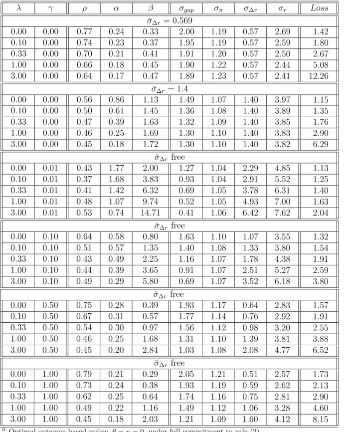
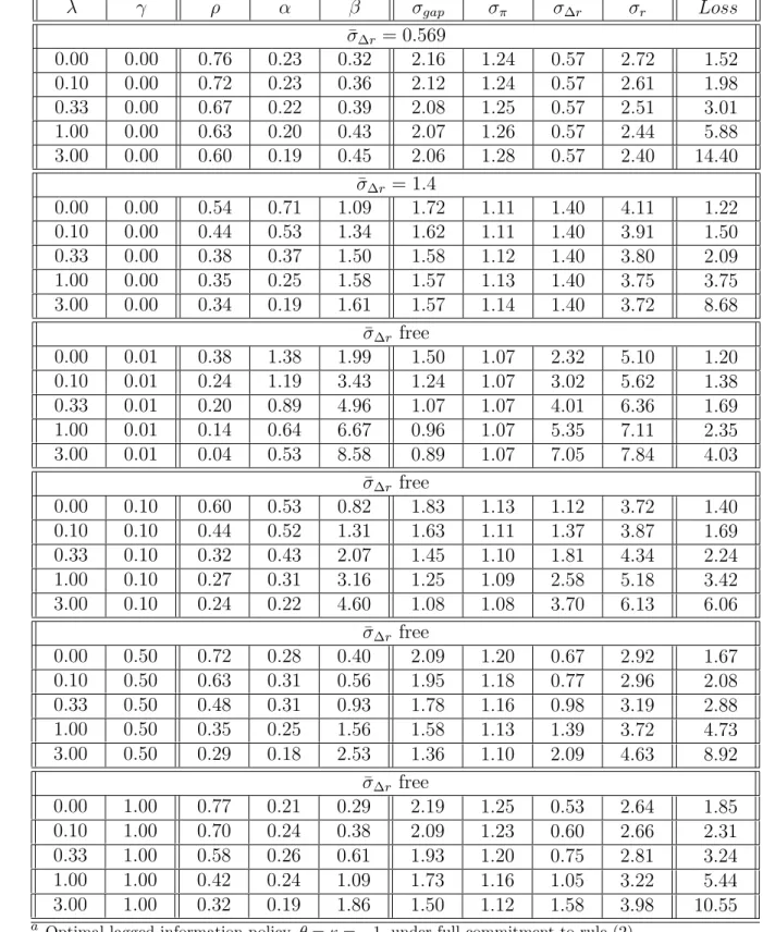
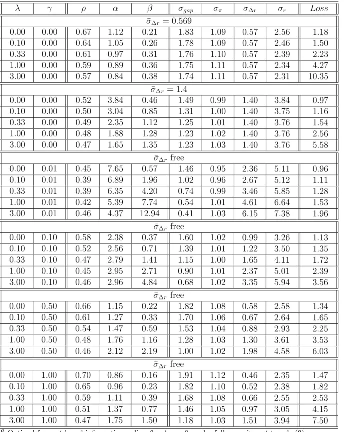
the empirical value). Table 2 summarizes the results for varying preferences for output gap stabilization if the contemporaneous Taylor Rule is used. Tables 3 and 4 report the results for the delayed informational assumption as well as for the forward-looking Taylor rule.

At extremes, we consider the case of strict inﬂation targeting,λ = 0, and preferences geared towards output-gap targeting, λ = 3.16 Smoothing parameters (ρ) for all

informa-positive. Their argument is that since output is a useful predictor of future inflation there is implicit “output-encompassing” in this case. A longer inflation forecast horizon brings inflation back to target more gradually dampening the amplitude of the real side on the outset of supply shocks. Varyingθ alone then varies the degree of encompassing. Levinet al. (2003) have an empirical counter-example where settingβ= 0 considerably deteriorates stabilization performance.

15_Levin_{et al.}_{(1999) argue that high frequency noise may lead the policymaker not to base his interest}

rate decisions on quarterly inflation information but rather on annual inflation in order to average this noise out. We examined this argument for a subset of simple rules. For contemporaneous rules there is a slight advantage of using annual information in the feedback rules. For forecast-based rules (θ= 4) this advantage vanishes as one would have expected since in forming expectations high-frequency noise does not play any role (the model is linear and shocks are additive white noise). In addition, expected quarterly inflation a year ahead is better controllable than expected annual inflation a year ahead, as the latter includes the intermediate quarterly inflation rates which are harder to influence due to policy lags. Qualitative results, however, did not seem to depend much on this choice.

(22)

Table 2: Optimized Policy Under Contemporaneous Rulea λ γ ρ α β σgap σπ σ∆r σr Loss ¯ σ_∆r= 0.569 0.00 0.00 0.77 0.24 0.33 2.00 1.19 0.57 2.69 1.42 0.10 0.00 0.74 0.23 0.37 1.95 1.19 0.57 2.59 1.80 0.33 0.00 0.70 0.21 0.41 1.91 1.20 0.57 2.50 2.67 1.00 0.00 0.66 0.18 0.45 1.90 1.22 0.57 2.44 5.08 3.00 0.00 0.64 0.17 0.47 1.89 1.23 0.57 2.41 12.26 ¯ σ_∆r = 1.4 0.00 0.00 0.56 0.86 1.13 1.49 1.07 1.40 3.97 1.15 0.10 0.00 0.50 0.61 1.45 1.36 1.08 1.40 3.89 1.35 0.33 0.00 0.47 0.39 1.63 1.32 1.09 1.40 3.85 1.76 1.00 0.00 0.46 0.25 1.69 1.30 1.10 1.40 3.83 2.90 3.00 0.00 0.45 0.18 1.72 1.30 1.10 1.40 3.82 6.29 ¯ σ_∆r free 0.00 0.01 0.43 1.77 2.00 1.27 1.04 2.29 4.85 1.13 0.10 0.01 0.37 1.68 3.83 0.93 1.04 2.91 5.52 1.25 0.33 0.01 0.41 1.42 6.32 0.69 1.05 3.78 6.31 1.40 1.00 0.01 0.48 1.07 9.74 0.52 1.05 4.93 7.00 1.63 3.00 0.01 0.53 0.74 14.71 0.41 1.06 6.42 7.62 2.04 ¯ σ_∆r free 0.00 0.10 0.64 0.58 0.80 1.63 1.10 1.07 3.55 1.32 0.10 0.10 0.51 0.57 1.35 1.40 1.08 1.33 3.80 1.54 0.33 0.10 0.43 0.49 2.25 1.16 1.07 1.78 4.38 1.91 1.00 0.10 0.44 0.39 3.65 0.91 1.07 2.51 5.27 2.59 3.00 0.10 0.49 0.29 5.80 0.69 1.07 3.52 6.18 3.80 ¯ σ_∆r free 0.00 0.50 0.75 0.28 0.39 1.93 1.17 0.64 2.83 1.57 0.10 0.50 0.67 0.31 0.57 1.77 1.14 0.76 2.92 1.91 0.33 0.50 0.54 0.30 0.97 1.56 1.12 0.98 3.20 2.55 1.00 0.50 0.46 0.25 1.68 1.31 1.10 1.39 3.81 3.88 3.00 0.50 0.45 0.20 2.84 1.03 1.08 2.08 4.77 6.52 ¯ σ_∆r free 0.00 1.00 0.79 0.21 0.29 2.05 1.21 0.51 2.57 1.73 0.10 1.00 0.73 0.24 0.38 1.93 1.19 0.59 2.62 2.13 0.33 1.00 0.62 0.25 0.64 1.74 1.16 0.75 2.81 2.90 1.00 1.00 0.49 0.22 1.16 1.49 1.12 1.06 3.28 4.60 3.00 1.00 0.45 0.18 2.03 1.21 1.09 1.60 4.12 8.15 a

Optimal outcome-based policy,θ=κ= 0,under full commitment to rule (2).

(23)

Table 3: Optimized Policy Under Lagged Rulea λ γ ρ α β σgap σπ σ∆r σr Loss ¯ σ_∆r= 0.569 0.00 0.00 0.76 0.23 0.32 2.16 1.24 0.57 2.72 1.52 0.10 0.00 0.72 0.23 0.36 2.12 1.24 0.57 2.61 1.98 0.33 0.00 0.67 0.22 0.39 2.08 1.25 0.57 2.51 3.01 1.00 0.00 0.63 0.20 0.43 2.07 1.26 0.57 2.44 5.88 3.00 0.00 0.60 0.19 0.45 2.06 1.28 0.57 2.40 14.40 ¯ σ_∆r = 1.4 0.00 0.00 0.54 0.71 1.09 1.72 1.11 1.40 4.11 1.22 0.10 0.00 0.44 0.53 1.34 1.62 1.11 1.40 3.91 1.50 0.33 0.00 0.38 0.37 1.50 1.58 1.12 1.40 3.80 2.09 1.00 0.00 0.35 0.25 1.58 1.57 1.13 1.40 3.75 3.75 3.00 0.00 0.34 0.19 1.61 1.57 1.14 1.40 3.72 8.68 ¯ σ_∆r free 0.00 0.01 0.38 1.38 1.99 1.50 1.07 2.32 5.10 1.20 0.10 0.01 0.24 1.19 3.43 1.24 1.07 3.02 5.62 1.38 0.33 0.01 0.20 0.89 4.96 1.07 1.07 4.01 6.36 1.69 1.00 0.01 0.14 0.64 6.67 0.96 1.07 5.35 7.11 2.35 3.00 0.01 0.04 0.53 8.58 0.89 1.07 7.05 7.84 4.03 ¯ σ_∆r free 0.00 0.10 0.60 0.53 0.82 1.83 1.13 1.12 3.72 1.40 0.10 0.10 0.44 0.52 1.31 1.63 1.11 1.37 3.87 1.69 0.33 0.10 0.32 0.43 2.07 1.45 1.10 1.81 4.34 2.24 1.00 0.10 0.27 0.31 3.16 1.25 1.09 2.58 5.18 3.42 3.00 0.10 0.24 0.22 4.60 1.08 1.08 3.70 6.13 6.06 ¯ σ_∆r free 0.00 0.50 0.72 0.28 0.40 2.09 1.20 0.67 2.92 1.67 0.10 0.50 0.63 0.31 0.56 1.95 1.18 0.77 2.96 2.08 0.33 0.50 0.48 0.31 0.93 1.78 1.16 0.98 3.19 2.88 1.00 0.50 0.35 0.25 1.56 1.58 1.13 1.39 3.72 4.73 3.00 0.50 0.29 0.18 2.53 1.36 1.10 2.09 4.63 8.92 ¯ σ_∆r free 0.00 1.00 0.77 0.21 0.29 2.19 1.25 0.53 2.64 1.85 0.10 1.00 0.70 0.24 0.38 2.09 1.23 0.60 2.66 2.31 0.33 1.00 0.58 0.26 0.61 1.93 1.20 0.75 2.81 3.24 1.00 1.00 0.42 0.24 1.09 1.73 1.16 1.05 3.22 5.44 3.00 1.00 0.32 0.19 1.86 1.50 1.12 1.58 3.98 10.55 a

(24)

Table 4: Optimized Policy Under Forecast-Based Rulea λ γ ρ α β σgap σπ σ∆r σr Loss ¯ σ_∆r= 0.569 0.00 0.00 0.67 1.12 0.21 1.83 1.09 0.57 2.56 1.18 0.10 0.00 0.64 1.05 0.26 1.78 1.09 0.57 2.46 1.50 0.33 0.00 0.61 0.97 0.31 1.76 1.10 0.57 2.39 2.23 1.00 0.00 0.59 0.89 0.36 1.75 1.11 0.57 2.34 4.27 3.00 0.00 0.57 0.84 0.38 1.74 1.11 0.57 2.31 10.35 ¯ σ_∆r = 1.4 0.00 0.00 0.52 3.84 0.46 1.49 0.99 1.40 3.84 0.97 0.10 0.00 0.50 3.04 0.85 1.31 1.00 1.40 3.75 1.16 0.33 0.00 0.49 2.35 1.12 1.25 1.01 1.40 3.76 1.54 1.00 0.00 0.48 1.88 1.28 1.23 1.02 1.40 3.76 2.56 3.00 0.00 0.47 1.65 1.35 1.23 1.03 1.40 3.76 5.58 ¯ σ_∆r free 0.00 0.01 0.45 7.65 0.57 1.46 0.95 2.36 5.11 0.96 0.10 0.01 0.39 6.89 1.96 1.02 0.96 2.67 5.12 1.11 0.33 0.01 0.39 6.35 4.20 0.74 0.99 3.46 5.85 1.28 1.00 0.01 0.42 5.39 7.74 0.54 1.01 4.61 6.64 1.53 3.00 0.01 0.46 4.37 12.94 0.41 1.03 6.15 7.38 1.96 ¯ σ_∆r free 0.00 0.10 0.58 2.38 0.37 1.60 1.02 0.99 3.26 1.13 0.10 0.10 0.52 2.56 0.71 1.39 1.01 1.22 3.50 1.35 0.33 0.10 0.47 2.79 1.41 1.15 1.00 1.65 4.11 1.72 1.00 0.10 0.45 2.95 2.71 0.90 1.01 2.37 5.01 2.39 3.00 0.10 0.46 2.96 4.84 0.68 1.02 3.35 5.94 3.56 ¯ σ_∆r free 0.00 0.50 0.66 1.15 0.22 1.82 1.08 0.58 2.58 1.34 0.10 0.50 0.61 1.27 0.33 1.70 1.06 0.67 2.64 1.65 0.33 0.50 0.54 1.47 0.59 1.53 1.04 0.88 2.93 2.25 1.00 0.50 0.48 1.76 1.16 1.28 1.03 1.30 3.61 3.53 3.00 0.50 0.46 2.12 2.19 1.00 1.02 1.98 4.58 6.03 ¯ σ_∆r free 0.00 1.00 0.70 0.86 0.16 1.91 1.12 0.46 2.35 1.47 0.10 1.00 0.65 0.96 0.23 1.82 1.10 0.52 2.38 1.82 0.33 1.00 0.59 1.11 0.39 1.68 1.08 0.66 2.55 2.53 1.00 1.00 0.51 1.37 0.77 1.46 1.05 0.97 3.05 4.15 3.00 1.00 0.47 1.75 1.50 1.18 1.03 1.51 3.94 7.50 a

(25)

tional assumptions are rather small, ranging between 0.04 and 0.79 across preferences and policy rules. These values are thus far from unity even for a strict inflation target – in contrast to the results of Levinet al. (1999, 2003) for Federal Reserve Board models. The features of the AWM outlined in section 3 provide some explanations: first, abstracting from the intrinsic persistence in inflation and the output gap, long-term interest rates and expectations do not play a dominant role in the AWM. The commitment value of persis-tent changes in the real rates is not substantial enough so as to merit strong additional smoothing. Second, as highlighted in section 3 even a rule with modest smoothing can imply substantial smoothing of the policy instrument in the reduced form of the model due to the model’s intrinsic persistence. In light of the less pronounced smoothing found here, it is not surprising that the integral control or first-difference rule purported in Levin

et al. (2003) to be robust to model uncertainty, does not even succeed in stabilizing the economy but results in an explosive equilibrium. These results for the AWM square with the evidence of Batini and Nelson (2001), Cˆot´eet al. (2002) as well as Levin and Williams (2003): in the more backward-looking and persistent models smoothing is less pronounced and excessive smoothing may severely deteriorate stabilization.

Another notable feature is that within each class of policies, the possible percentage reductions in output variability and inﬂation variability both are small, being close to 5% and 3%, respectively, for the case of the empirical upper bound. For the contemporaneous outcome-based rule, for example, output variability is reduced by 5.3% when moving from toλ = 0 toλ= 3, while inﬂation volatility is only reduced by 3.1% going in the opposite direction. However, this does not mean that there is barely any menu choice for the policymaker: comparing the economic stability under the optimal rules to the performance under the given rules in Table 1 highlights that there is a substantial stabilization gain arising from optimal monetary policy.

Allowing for more flexibility in interest rates shows that the AWM implies that the largest gain from stabilization can be imparted on the output gap while the reduction in inflation variability is comparatively mild. For instance, for the contemporaneous Taylor rule with an upper bound on interest rate change volatility of 1.4, output variability is reduced by 15% while inflation variability only increases by roughly 3%. On the one hand, there may be a strong “exogenous” component in the price dynamics, on the other, given the long cycles in output illustrated in figures 1 through 4, curbing real side variability

(26)

may contribute substantially towards stabilizing inflation.Imposing no strict upper bound on interest change variability, but rather implementing a penalty term γ > 0 in the loss function illustrates that there is a strong trade-off between stabilizing the output gap and stabilizing the interest rate, while again the trade-off for inflation stabilization is rather mild.17 _{As argued in section 2, the implications of optimal discretionary policy provide a}

natural benchmark – reported in Table 5.

Figure 6 highlights for the case of the empirical upper bound that there is hardly any “menu choice” within each set of policies for the policymaker once conducting optimal pol-icy. However, as we plot the efficiency frontiers for the policies considered herein, there are substantial stabilization differences across classes of policies. The respective northwesterly part of the frontiers pertains to an inflation targeting central bank while the southeast refers to almost pure output gap targeting. Three observations are apparent: first, using current information is substantially preferred to using lagged information. Second, for the arbitrary choice of a one-year forecast horizon for inflation, forecast-based policy strictly dominates outcome-based policy. Third, there is substantial value added of incorporating all information into the model as highlighted by the stabilization performance of optimal discretionary policy. For empirical comparison, we also show two rules recently estimated for the Euro area: Gerdesmeier and Roffia’s (2003) rule with contemporaneous inflation and Gerlach and Schnabel’s (2000) rule with a forecast based inflation term. While in the AWM these imply slightly larger interest rate variability than observed in the data, they can nevertheless serve as a rough benchmark for the simple optimal rules. In particular, the Gerdesmeier and Roffia rule puts insufficient weight on the output gap and hence does considerably worse than the optimal contemporaneous outcome-based rule. In contrast, by visual inspection, the rule estimated by Gerlach and Schnabel, although incorporating insufficient smoothing, comes closer to the optimal frontier for forecast-based policy.

Simple rules may be argued to be easy to monitor so the central bank may be able to commit to them credibly. However, being contingent only on a small subset of states,

17_{This may even look inverted,}_i.e._{as if inﬂation variability would be decreasing in the weight on output}

stability. However, increasing λ alters both the inflation-output gap stabilization trade-off and the trade-off between stabilizing either of these and smoothing the interest rate. Namely the latter is relatively less costly when λ is increased, rendering decreases of inflation variability if λ increases plausible.

(27)

Table 5: Results for Optimal Discretionary Policya λ γ σgap σπ σ_∆r σr Loss ¯ σ_∆r= 0.569 0.00 0.00 1.66 1.01 0.57 2.39 1.01 0.10 0.00 1.55 1.01 0.57 2.28 1.27 0.33 0.00 1.49 1.03 0.57 2.22 1.80 1.00 0.00 1.47 1.05 0.57 2.18 3.27 3.00 0.00 1.47 1.06 0.57 2.16 7.61 ¯ σ_∆r = 1.4 0.00 0.00 1.59 0.95 1.40 3.81 0.91 0.10 0.00 1.21 0.97 1.40 3.59 1.08 0.33 0.00 1.10 0.99 1.40 3.60 1.38 1.00 0.00 1.07 1.01 1.40 3.61 2.15 3.00 0.00 1.06 1.02 1.40 3.61 4.42 ¯ σ_∆r free 0.00 0.01 1.64 0.94 2.11 4.84 0.92 0.10 0.01 1.04 0.95 2.40 4.74 1.07 0.33 0.01 0.75 0.98 3.17 5.50 1.24 1.00 0.01 0.54 1.01 4.32 6.34 1.49 3.00 0.01 0.41 1.03 5.86 7.14 1.91 ¯ σ_∆r free 0.00 0.10 1.61 0.98 0.82 2.87 1.03 0.10 0.10 1.34 0.98 1.00 3.02 1.24 0.33 0.10 1.10 0.99 1.41 3.62 1.58 1.00 0.10 0.86 1.00 2.10 4.54 2.19 3.00 0.10 0.66 1.02 3.06 5.53 3.30 ¯ σ_∆r free 0.00 0.50 1.70 1.02 0.47 2.19 1.16 0.10 0.50 1.57 1.02 0.54 2.22 1.43 0.33 0.50 1.40 1.01 0.71 2.48 1.94 1.00 0.50 1.19 1.01 1.09 3.12 3.04 3.00 0.50 0.96 1.02 1.72 4.07 5.26 ¯ σ_∆r free 0.00 1.00 1.75 1.05 0.38 1.98 1.24 0.10 1.00 1.65 1.04 0.42 1.98 1.53 0.33 1.00 1.52 1.03 0.53 2.14 2.12 1.00 1.00 1.33 1.03 0.79 2.60 3.46 3.00 1.00 1.10 1.02 1.28 3.43 6.35

a _{Optimal discretionary policy under full information. See Appendix}

(28)

1 1.05 1.1 1.15 1.2 1.25 1.3 1.35 1.4 1.4 1.5 1.6 1.7 1.8 1.9 2 2.1 2.2 2.3 2.4 σ(π) σ (y) Gerdesmeier−Roffia lagged contemporaneous Gerlach−Schnabel forecast−based discretion

Figure 6: Optimal Policy Frontiers. Shown is the locus of combinations of standard deviations of the output gap (vertical axis) and standard deviations of inﬂation (horizontal axis) for the optimized simple lagged (dotted) and contemporaneous (solid) outcome-based rules as well as for the forecast-based (dash-dotted) rule with a horizons θ = 4, κ= 0 for the empirical upper bound on interest rate change variability. In addition, we plot the locus implied by rules (4) and (6). The frontier implied by optimal policy under discretion is shown as a dashed line.

these are neither fully optimal nor necessarily time-consistent in the absence of some commitment technology. While it is commonly found that the commitment value provided by credible Taylor rules outweighs the loss incurred by conditioning policy only on a subset of information, this ranking depends on model characteristics. Most notably the greater is the information content of other states in the economy (besides the output gap, interest rates and inﬂation) and the less important is the expectations channel (in the extreme, in a backward-looking model, there is no distinction between Discretion and Commitment), the more valuable will be optimal time-consistent policy as opposed to sub-optimal (simple optimal) policy under commitment. We provide the optimal discretionary solution as a natural benchmark in the spirit of inﬂation targeting as promoted by Svensson (1999a).

(29)

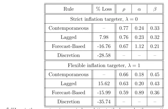
For the AWM, due to its highly persistent and rich structure, the information gain by far outweighs the credibility loss when we compare the simple optimal frontiers to the optimal discretionary frontier. Consequently, one might conjecture, that the information encompassing property of the forecast-based rules explains most of the gains relative to contemporaneous rules. In contrast to other authors, such as Levin et al. (2003), we ﬁnd the gains from implementing forecast-based policy to be marked. Table 6 presents

Table 6: Relative Lossesa

Rule % Loss ρ α β

Strict inﬂation targeter, λ= 0

Contemporaneous – 0.77 0.24 0.33 Lagged 7.98 0.76 0.23 0.32 Forecast-Based -16.76 0.67 1.12 0.21 Discretion -28.58 – – –

Flexible inﬂation targeter, λ= 1

Contemporaneous – 0.66 0.18 0.45 Lagged 15.62 0.63 0.20 0.43 Forecast-Based -15.99 0.59 0.89 0.36 Discretion -35.74 – – –

a _{%Loss is the percentage increase in loss relative to the loss under the respective optimized simple}

contemporaneous rule for λ = 0 and λ = 1, respectively. The Table refers to the results with an empirical upper bound of ¯σ_∆_r= 0.569 on interest rate change variability.

numerical values for the relative losses and illustrates that the gain from implementing forecast-based policy is roughly 17% relative to implementing an optimized Taylor rule feeding back on contemporaneous inflation. Discretionary policy using all states of the model by far outperforms the simple rules under commitment (a reduction in losses of roughly 29% relative to contemporaneous Taylor rules). This highlights that there is a substantial amount of information in the model for which inflation and the output gap are not sufficient statistics. While the exchange rate as demonstrated in (McAdam and Morgan, 2003), plays a key role in the model, and thereby its expectations, the

(30)

not feeding back on all states. 18

As Table 2 highlights, for outcome-based Taylor rules, the weightβ on the output gap is always larger than the weight on the inflation term even for a strictly inflation targeting central bank. While output is not a target variable in that case, it will in light of the impulse response evidence of section 3 be a good indicator variable for expected future inflation, which given policy lags ultimately is what the central bank is able to influence. Consequently, the weight on the output gap term decreases substantially relative to the inflation weight, when the policymaker is allowed to directly react to expected inflation.

Our results so far highlight ﬁrst, that simple rules can do much worse than optimal discretionary policy. After all, in a more backward-looking but persistent framework, where most of the variables are pre-determined, the central bank needs to take most of those into account for optimal policy conduct. Second, in line with these results, the forward-looking Taylor rules provide a remarkable improvement above outcome-based rules. We attribute these results to the information-encompassing provided by the ratio-nal expectations in the rule. Despite the apparent structural simplicity of the simple rules, for practical policy implementation several caveats seem to be in order. The outcome-based rules are easily implemented only if one abstracts from the uncertainty surrounding (real-time) output gap estimates. In addition, expectations in the policy rule and in the model are taken to be model consistent rational expectations. Among other things, this amounts to the assumption that private sector forecasts are derived using the central bank’s structural (Area-Wide) model – which may be violated in the face of model un-certainty. While this assumption also has a bearing on the optimal parameter values of the rules, its importance may be most obvious for forecast based rules. Consequently, to guard against private sector expectations not being in line with central bank forecasts, one may be tempted to resort to survey forecasts instead of applying model-consistent forecasts. Bernanke and Woodford (1997), however, illustrate that things are not that straightforward. In particular, directly targeting survey private sector expectations would

18_{From a theoretical angle, Svensson (2000) has argued that foreign variables should also appear as}

feedback parameters in open economy Taylor rules. From an empirical perspective Claridaet al.(1998) illustrate that real exchange rates and foreign funds rates could be significant ingredients to the optimized simple rule, although they have small quantitative effects. Gerdesmeier and Roffia (2003) find that the real effective exchange rate is just marginally insignificant, while the significance of nominal exchange rates and the federal funds rate is refuted more soundly. Upon a first exploration we did not find a few contemporaneous variables capturing the bulk of information in the model. We

(31)

likely nullify the information content of these measures and thereby lead the procedure

ad absurdum leaving the equilibrium open to indeterminacy. Ultimately then, monetary authorities must rely on an explicit structural model of the economy to guide their policy decisions, as we do here, and cannot point at the simplicity of these rules.

In section 5, we derive optimal forecast horizons for forecast-based policy rules. We will illustrate that there is significant gain from an optimal choice of the horizon both for inflation as well as for the output gap forecast. Intuitively speaking, this feature arises due to the exploitation of all model states (although in a restricted manner). Before turning to the optimal horizons we briefly highlight the role of commitment in the AWM.

4.2 Benchmarking Against Commitment

Conducting optimal policy under commitment may not be feasible for the policymaker as it becomes problematic for the outside world to monitor policy whenever it conditions on a large set of states. For the sake of completeness, we highlight the role for more com-plicated commitment policy in the AWM. Commitment is by definition enhancing over simple rules (given that it potentially encompasses all states) and should also (though to a lesser extent) dominate the discretionary solution. We found pronounced difficulties in solving for the fully optimal commitment solution and considered that our results for that solution may not be particularly robust to the way the transmission of structural shocks has been identified.19 _{We resort to an approximation of the first best commitment}

solution. Giannoni and Woodford (2003) have shown theoretically that the optimal com-mitment policy can be approximated closely by a generalized Taylor rule which in addition to the contemporaneous feedback contains enough lags and expectational leads of the tar-get variables themselves. While for smaller more forward-looking models the number of lags and leads needed is rather contained, apparently this is not the case for a model

19_{As regards the computation, the AWM even after linearization is nearly non-stationary due to the}

“exogenous” processes. For numeric reasons, it is impossible to solve the model augmented by the costates as in Dennis (2001) by AIM. When resorting to Sims’ (2001) procedure, the determinacy conditions yield one loose endogenous error, rendering the equilibrium indeterminate. As Lubik and Schorfheide (2003) highlight, in that case not only might sunspot shocks effect the economy, but also the transmission of structural shocks through the model is not uniquely determined. We overrode the indeterminacy issue and used the identification provided by Sims. This resulted in discretion being 20% to 70% worse than commitment. These values are larger than in the literature and somewhat surprising given the limited role of expectations in the AWM. Since these results suffer from the identification problem mentioned above, we do not consider these to be reliable. For completeness, we nevertheless report these results in Appendix F.

(32)

incorporating a complicated lag structure like the AWM. For one set of preferences, Table 7 displays the losses involved when committing to an optimized rule with a total of ten lags and three expectational leads – and hence 41 free parameters. The ﬁnal row reports results for four lags and six leads. As is apparent, the gains over optimal discretionary

Table 7: Pseudo-Commitmenta λ γ σgap σπ σ∆r σr Loss ¯ σ_∆r free 0.00 0.50 1.71 1.02 0.46 2.17 1.15 0.10 0.50 1.58 1.02 0.53 2.22 1.42 0.33 0.50 1.40 1.01 0.71 2.50 1.94 1.00 0.50 1.19 1.01 1.09 3.14 3.04 3.00 0.50 0.96 1.01 1.73 4.10 5.26 1.00 0.50 1.19 1.01 1.09 3.15 3.03

a _{The Table reports results for pseudo-commitment. The rules include 10 lags and 3 expectational leads}

of the target variablesgap, π, ∆r.The exception is the last line, which entertains 4 lags and 6 leads.

policy are mild at best. Even complicated rules as these do not improve greatly upon the discretionary policy and fall far short of the commitment results reported in appendix F that appear when using Sims’ (2001) identiﬁcation of endogenous and exogenous shocks. In the framework of the AWM, with a large set of states and high intrinsic persistence paired with limited forward-lookingness, even such highly complicated rule-based com-mitment policy does not improve considerably on the discretionary outcome. To us, this highlights once more that in such an environment, it is extremely important to capture the information content in all state variables.20 _{For a comparison, Finan and Tetlow}

(1999) report for the more forward-looking FRB/US model, which features roughly 300 equations, that a simple optimized contemporaneous Taylor rule is between 14% to 25% worse than the optimal commitment solution. If we take the pseudo-commitment rules as close enough approximation to fully optimal commitment, results for the AWM range at the upper limit of this interval owing to the strong persistence and limited

forward-20 _{Optimizing 41 parameters already turns out to be computationally expensive. As the above exercise}

serves mainly illustrative purposes, we report results only for one set of preferences. In addition, we refrain from approximating commitment policy more closely by adding more leads and lags to the rules. Accordingly, we do not claim that the results reported constitute the global optimum under commitment but rather term the long rules “pseudo-commitment.”

(33)

lookingness of the model. As Table 8 illustrates, optimal simple rules can increase losses by roughly 27% relative to pseudo-commitment. Again, that the deterioration from using

Table 8: Relative Losses for γ = 0.5a

Rule % Loss σgap σπ σ_∆r σr

Strict inﬂation targeter, λ= 0

Contemporaneous – 1.93 1.17 0.64 2.83 Lagged 6.37 2.09 1.20 0.67 2.92 Forecast-Based -14.64 1.82 1.08 0.58 2.58 Discretion -26.11 1.70 1.02 0.47 2.19 Pseudo-Commitment -26.75 1.71 1.02 0.46 2.17

Flexible inﬂation targeter, λ= 1

Contemporaneous – 1.31 1.10 1.39 3.81 Lagged 21.9 1.58 1.13 1.39 3.72 Forecast-Based -9.02 1.28 1.03 1.30 3.61 Discretion -21.6 1.19 1.01 1.09 3.12 Pseudo-Commitment -21.6 1.19 1.01 1.09 3.14

Given Policy Rules, λ= 0 (λ = 1)

Taylor 70.9(75.4) 2.03 1.23 1.53 2.33 Gerdesmeier-Roﬃa 32.5 (103.3) 2.41 1.36 0.68 2.44 Claridaet al. 27.9 (88.1) 2.30 1.39 0.39 1.70 Gerlach-Schnabel 1.3 (34.0) 1.90 1.18 0.63 1.85

a _{%Loss is the percentage increase in loss relative to the loss under the respective optimized simple}

contemporaneous rule for λ = 0 and λ = 1, respectively. The Table refers to the results with a punishmentγ= 0.5 on interest rate change variability.

less complicated rules is at times sizeable can be attributed to the fact that the AWM is very much persistent.

A conclusion emerging from the results of this section is that the Central Bank if it is willing to condition its policy on the AWM framework should take all available information into account even if this results in very complicated interest rate rules. We next turn to illustrate the gains to forward-looking policy in a framework as the AWM.

(34)

5 Optimal Forecast Horizons

The more forward-looking a model, the more agents take into account both current and future policy conditions, thereby in eﬀect reducing the importance of policy lags and the uncertainty surrounding them. In contrast, as Batini and Nelson (2001) highlight, in backward-looking models, i.e., in the absence of an expectations channel or with a large degree of intrinsic persistence, policy lags may be longer thereby leading to an optimal forecast horizon farther into the future. With too long a forecast horizon, however, indeterminacy can occur for any value of the feedback parameters as argued by Batini et al. (2003).21 _{We turn to the issue of optimal forecast horizons in due course focusing on}

the benefits of choosing an optimal inflation forecast horizon first (which has been most intensively emphasized in the literature so far).

5.1 Optimal Forecast Horizons for Inflation

We minimize loss function (1) with respect to the feedback parametersρ, αandβ and dis-cretely for the forecast horizon θ for a policy-maker who credibly implements the forecast based rule

rt=ρrt−1 +αEtπt+θ+βgapt, θ ∈ {1,2, ...,16}. (7)

As we seek to derive conclusions closest to the current policy regime as possible and in order not to overload the current paper, we focus exclusively on the case with an empirical upper bound on interest change variability. Table 9 summarizes the results, which figure 7 illustrates graphically. The optimal forecast horizon for a strictly inflation targeting central bank is θ = 10 quarters. The optimal forecast horizon is associated with a loss only 1.2% larger than the corresponding loss under discretion and full information, compared to a 16.5% larger loss with a conventional one year forecast horizon. A sizeable portion of model information can thus be incorporated by means of inflation forecast-based rules with an optimally chosen horizon. For a policy-maker who weights output gap stabilization, λ = 1₃, the optimal horizon, θ,is at 11 quarters. The loss in distance in

21_{With constant interest rates, the AWM is stationary, but the equilibrium is indeterminate – there are}

an infinite number of paths on which the economy can converge to the stable growth path. In the stationary environment, as the forecast horizons tend to infinity, the expectations of inflation and the output gap converge to their unconditional expectations, zero. Interest rates then are exogenous and constant.