Trading Down and the Business Cycle
∗
Nir Jaimovich
†, Sergio Rebelo
‡, and Arlene Wong
§October 2017
Abstract
We document two facts. First, during the Great Recession, consumers traded down in the quality of the goods and services they consumed. Second, the produc-tion of low-quality goods is less labor intensive than that of high-quality goods. When households traded down, labor demand fell, increasing the severity of the recession. We find that the trading-down phenomenon accounts for a substan-tial fraction of the fall in U.S. employment in the recent recession. We show that embedding quality choice in a business-cycle model improves the model’s amplification and comovement properties.
J.E.L. Classification: E2, E3, E4.
Keywords: Recessions, quality choice, business cycles.
∗This research was conducted with restricted access to the Bureau of Labor Statistics (BLS) data. The views expressed here are those of the authors and do not necessarily reflect the views of the BLS. We thank our project coordinator at the BLS, Ryan Ogden, for help with the data, and Yuriy Gorodnichenko and Michael Weber for making their data and code available to us. We are grateful for comments from David Berger, Erik Hurst, Guido Menzio, Emi Nakamura, Aviv Nevo, Raphael Schoenle, Henry Siu, and Jon Steinsson.
†University of Zurich.
‡Northwestern University, NBER, and CEPR. §Princeton University and NBER.
1
Introduction
One of the classic research areas in macroeconomics is the study of how households make consumption choices and how these choices impact the economy. There is a large empirical literature on this topic going as far back as the work of Burns and Mitchell (1946). This literature has received renewed attention after the Great Recession.1
In this paper, we contribute to this line of research as follows. First, we show that during the Great Recession, consumers traded down in the quality of the goods and services they consumed. Second, we show that the production of low-quality goods is generally less labor intensive than that of high-quality goods. These two facts imply that when households traded down, labor demand fell, increasing the severity of the Great Recession.
To quantify the implications of “trading down” for employment during the Great Recession, we combine various data sources to construct a data set with firm-level measures of product quality, labor intensity, and market share. For most of our analysis, we use prices as a proxy for quality. Our assumption is that, if consumers are willing to pay more for an item, they perceive it to be of higher quality. We corroborate the plausibility of this assumption using data with independent measures of quality and price.
We obtain price measures from two sources: data scraped from the Yelp!, a website where consumers post information about different goods and services, and the confiden-tial micro data set used to construct the Producer Price Index (PPI). We merge these data with Compustat data to measure labor intensity and market share for each firm in our sample. We estimate that around half of the decline in employment in the Great Recession is accounted for by consumers trading down in the quality of the goods and services they purchased.
1Recent contributions to this literature include Aguiar, Hurst, and Karabarbounis (2013), Kaplan
To study the effects of trading down from a theoretical perspective, we embed quality choice into an otherwise standard business-cycle model. We find that the presence of quality choice magnifies the response of these economies to shocks, generating larger booms and deeper recessions. To understand this amplification mechanism consider a negative shock that reduces the household’s income. This fall in income, leads the household to trade down in the quality of the goods it consumes. Since lower quality goods use less labor, trading down reduces labor demand.
The quality-augmented model has two other interesting properties. First, it can generate comovement between employment in the consumption and investment sectors, a property that is generally difficult to obtain (see Christiano and Fitzgerald (1998)). Second, the model produces an endogenous, countercyclical labor wedge. As Shimer (2009) emphasises, this type of wedge is necessary in order to reconcile business-cycle models with the empirical behavior of hours worked.
Our paper is organized as follows. In Section 2, we describe our data and present our empirical results. We study the quantitative properties of two models with quality choice in Section 3. The first model has a representative agent while the second has heterogenous agents. Section 4 concludes.
2
Empirical findings
In this section, we analyze the impact of trading down on labor demand. By trading down we mean shifts in the composition of consumption across firms within narrowly defined sectors towards lower quality goods. To study the effect of trading down on em-ployment, we estimate the labor intensity of different quality levels within each sector. We then study how shifts in the market share of the different quality levels affects em-ployment. This within-sector trading-down channel differs from other channels through which demand can affect employment, such as shifts in spending across sectors (e.g.
from restaurants to the grocery sector) or declines in total spending.2
Our empirical approach to study the effects of trading down is as follows. We denote byM the number of sectors in the economy. Total aggregate employment across these sectors is: Ht= M X m=1 Hm,t, (1)
whereHm,t denotes employment at time t in sector m.
In each sector, goods can belong to one of J levels of quality. The market share of quality tier j in sector m (Sj,m,t) is the ratio of sales of goods in quality tier j (Yj,m,t)
to total sales in sectorm (Ym,t):
Sj,m,t=
Yj,m,t
Ym,t
.
The measure of labor intensity (LIj,m,t) that we construct is the ratio of employees
(Hj,m,t) to sales (Yj,m,t):
LIj,m,t =
Hj,m,t
Yj,m,t
.
Using this notation, we can write total employment in sectorm in period t as: Hm,t =Ym,t
J
X
j=1
Sj,m,tLIj,m,t, (2)
whereYm,t denotes total sales in sectorm,Ym,t =
PJ
j=1Yj,m,t. Combining equations (1)
and (2), we can write aggregate employment as:
Ht=Yt M X m=1 Ym,t Yt J X j=1 Sj,m,tLIj,m,t, (3)
whereYtdenotes aggregate sales across theM sectors. Using equation (3), we can write 2See Section 2.5 for a discussion of shifts in spending across sectors.
the log-percentage change in employment, log(Ht+1/Ht) as:
log(Ht+1/Ht) = log (Yt+1/Yt) + log M X m=1 Ym,t+1 Yt+1 J X j=1 Sj,m,t+1LIj,m,t+1 ! −log M X m=1 Ym,t Yt J X j=1 Sj,m,tLIj,m,t ! . (4)
In order to quantify the effect of trading down on employment, we calculate a counterfactual value for employment in periodt+ 1:
HtCF+1 =Yt+1 M X m=1 Ym,t+1 Yt+1 J X j=1 Sj,m,tLIj,m,t+1 ! . (5)
This counterfactual level of employment is the one that would have occurred in the absence of trading down, that is, if the market shares of each quality tier were the same at timet and t+ 1.
In the absence of trading down, the percentage change in employment would have been:
log(HtCF+1/Ht) = log (Yt+1/Yt) + log M X m=1 Ym,t+1 Yt+1 J X j=1 Sj,m,tLIj,m,t+1 ! (6) −log M X m=1 Ym,t Yt J X j=1 Sj,m,tLIj,m,t ! .
The difference between the actual change in employment and the counterfactual change in employment if no trading down occurred, gives us an estimate of the im-portance of the trading down phenomenon for employment. Below, we produce this estimate using our data.
2.1
Empirical measures
We start by using a data set that merges information from Yelp!, the Census of Retail Trade, and Compustat. We then extend our analysis to the manufacturing sector by
using the micro data gathered by the BLS to construct the PPI. Finally, we consider several other data sets.
We define the relative quality of goods and services as encompassing anything that consumers are willing to pay for. This notion of quality encompasses both the item itself, and the service or convenience of the product. For example, in restaurants, it includes both the meal and the ambience of the place. For grocery stores, it is not only the item sold but also the convenience and service of the store.
We measure quality using the price distribution of firms within each sector. This measure is the most comprehensive in terms of sectoral coverage, making our analysis consistent across all of the sectors that we consider.
2.2
Results obtained with Yelp! and Census of Retail Trade
data
In this section, we discuss the results we obtain using data from Yelp! and from the Census of Retail Trade. The combined data set covers five North American Indus-try Classification System (NAICS) sectors: apparel, grocery stores, restaurants, home furnishing, and general merchandise. These sectors represent 17 percent of private non-farm employment. As we discuss below, our analysis includes the effects of trading down on the demand for intermediate inputs from all sectors in the economy computed using the BLS input-output data.
We focus on two main time periods. Our recession period goes from 2007 to 2012. Our pre-recession period goes from 2004 to 2007.3 We use data for the period 2004-2007 to control for trends in trading down to try to isolate the cyclical component of trading down associated with the Great Recession.
3Even though the NBER determined that the recession ended in June 2009, average and median
household income continued to fall until 2012. In addition, employment recovered very slowly: in December 2012 employment was still 3 percent below its December 2007 level. In Appendix E, we report results when we use 2007-2009 as the recession period.
Yelp! data
For sectors other than General Merchandise, we collect information on prices by scraping data from Yelp!, a website where consumers share reviews about different goods and services. For each store and location pair, Yelp! asks its users to classify the price of the goods and services they purchased into one of four categories: $ (low), $$ (middle), $$$ (high), and $$$$ (very high). Since there are few observation in the very-high category, we merge the last two categories into a single high-price category.
We construct the Yelp! data set as follows (see Appendix A for more details). We first associate each firm (for example, Cost Plus, Inc.) with its brand names and retail chains (for example, Cost Plus owns the retail chain World Market). We find the Yelp! profile for each retail chain and brand in the 18 largest U.S. cities and collect the first match (for example, the first match for World Market in Chicago is the store on 1623 N. Sheffield Av.). We then compute the average price category across the first match for each of the 18 cities (to compute this average, we assign 1 to category low, 2 to middle and 3 to high).4
Consistent with the assumption that prices proxy for quality, we find that there is a positive correlation between the average rating and the average price in the Yelp! data.
U.S. Census of Retail Trade data
For General merchandise, the U.S. Census of Retail Trade splits firms into three price tiers that correspond to three different levels of quality: non-discount stores (high quality), discount department stores (middle quality), other general merchandise stores, including family dollar stores (low quality). For each of these three tiers, the Census provides information about employment and sales. We use this information to construct labor intensity measures and market shares. The Census categorization in the general merchandise store sector aligns with the Yelp! categorization of Compustat firms into
4The dispersion in price categories across cities is relatively small; it is rare for firms to be included
price categories, highlighting the consistency of our quality categorization across the different data sources.
Compustat data
We merge the price information for each firm in our Yelp! data set with data from Compustat on the number of employees, sales, operating expenses, and cost of goods sold. Our measure of labor intensity is the ratio of employees to sales. We focus on this measure because of its availability. The SEC requires that firms report the number of employees and, as a result, these data are available for all companies in Compustat. In contrast, only less than 1/4 of the firms in Compustat of firms report labor costs.5
Findings
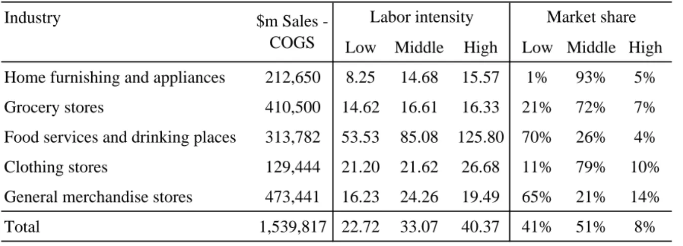
Tables 1 and 2 present our estimates of labor intensity and market share by quality tier. We use these estimates as inputs into equations (4) and (6). Labor intensity increases with quality in all five sectors. For example, in 2007, the number of employees per million dollar of sales is 6.33, 9.23 and 10.86 for low-, middle-, and high-quality apparel stores, respectively (Table 1). Overall, the middle quality uses 46 percent more workers per million dollar of sales than the low-quality producers. Similarly, the high-quality producers use 18 percent more workers per million dollar of sales than the middle-quality producers. Other things equal, a shift of one million dollar of sales from middle to a low quality stores reduces employment by roughly three jobs.
Between 2007 and 2012, firms that produce middle- and high-quality items lost market share relative to firms that produce low-quality items. In 2007, the low-,
middle-5For the sample of firms that report the labor share in cost, the correlation between labor share
and the labor intensity measure of employees/sales is 0.94. The correlation between the labor share in cost and employees/gross margin is 0.97. As a robustness check, we also use the ratio of employees to gross margin as a measure of labor intensity (Appendix D). Gross margin, which is sales minus cost of goods sold, is a measure that is close to value added. Value added is equal to the gross margin minus energy and services purchased. We cannot compute value added because Compustat does not report data on energy and services purchased. The correlation between employees/gross margin and employees/sales is 0.72.
and high-price categories account for 42, 52 and 6 percent of sales, respectively. In contrast by 2012, high-quality producers lost about 0.5 percentage points in market share, middle-quality producers lost 6.5 percentage points, and low-quality producers gained 7 percentage points. This pattern is present is all the sectors we consider with one exception: the market share of high-quality grocery stores increased. 6 This exception is driven by an outlier: WholeFoods, a high-quality supermarket that gained market share despite the recession.
With the information in Tables 1 and 2, we can implement the empirical approach described by equations (4) and (6). Overall employment in the sectors included in our data set fell by 3.39 percent. Using equation (6), we find that in the absence of trading down employment would have fallen by only 0.39 percent. This result implies that trading down accounts for (3.39−0.39)/3.39 = 88 percent of the fall in employment.7 Trend versus Cycle
Trading down was occurring before the recession, so there are both trend and cycle components of trading down. In order to disentangle these two components, we proceed as follows. We compute market shares by quality tier for each sector for the period 2004-2007. We use the change in these shares over this period to linearly extrapolate what the market shares of different quality tiers would have been in 2012. Using these market shares, we construct the 2012 employment implied by the extrapolated market shares
N2012CF2 =Y2012 5 X m=1 Ym,2012 Y2012 3 X j=1 Sj,m,2007+ Sj,m,2007−Sj,m,2004 (2007−2004) ×(2012−2007) [LIj,m,2012] ! . (7)
6Using the PPI data discussed below, we find that there is no correlation between the changes
in prices that occurred during the recession and the quality tier of the firm. This fact suggest that changes in market shares are driven mostly by changes in quantities rather than by changes in prices or markups. This inference is consistent with the finding in Anderson, Rebelo and Wong (2017) that markups in the retail sector remained relatively stable during the Great Recession.
7Our calculations are based on Census estimates of sector expenditures. We are implicitly assuming
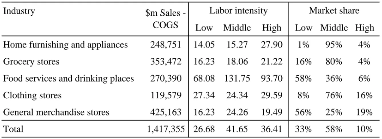
Table 1: Market shares and Labor Intensity: 2007
Industry $m Sales
Low Middle High Low Middle High
Home furnishing and appliances 654,535 4.40 4.97 7.10 1% 95% 5%
Grocery stores 547,837 3.37 4.68 7.58 39% 59% 2%
Food services and drinking places 444,551 15.63 24.02 22.43 52% 41% 7%
Clothing stores 221,205 7.55 9.43 16.49 11% 78% 11%
General merchandise stores 578,582 3.72 6.92 7.19 64% 23% 13%
Total 2,446,710 6.33 9.23 10.86 35% 58% 7%
Labor intensity Market share
Note: This table depicts the 2007 total sales, labor intensity and market share for different retail sectors. The last row is a sales-weighted measure. Sales are from the US Census of Retail Trade, and the labor intensities and market shares are from Compustat. Labor intensity is defined as the number of employees per million dollars of sales and the market share are the share of sales for each price tier within each sector. Price tiers are denoted by low, middle and high, and are based on Yelp! classifications of prices $, $$, and $$$, respectively. See text for more information.
Table 2: Market shares and Labor Intensity: 2012
Industry $m Sales
Census Low Middle High Low Middle High
Home furnishing and appliances 609,323 3.49 4.92 5.93 1% 94% 5%
Grocery stores 631,486 1.92 4.15 6.06 43% 53% 5%
Food services and drinking places 524,892 13.43 19.49 22.40 61% 33% 6%
Clothing stores 241,386 6.50 9.16 15.09 15% 77% 7%
General merchandise stores 649,754 3.72 6.92 7.19 72% 18% 10%
Total 2,656,841 5.41 8.49 10.36 42% 52% 6%
Labor intensity Market share
Note: This table depicts the 2012 total sales, labor intensity and market share for different retail sectors. The last row is a sales-weighted measure. Sales are from the US Census of Retail Trade, and the labor intensities and market shares are from Compustat. Labor intensity is defined as the number of employees per million dollars of sales and the market share are the share of sales for each price tier within each sector. Price tiers are denoted by low, middle and high, and are based on Yelp! classifications of prices $, $$, and $$$, respectively. See text for more information.
This counterfactual measure of employment is 2.38 percent lower than the level of employment in 2007. We conclude that (3.39−2.38)/3.39 = 30 percent of the fall in employment is due to trend factors. Recall that trading down accounted for a 3 percentage points fall in employment, so the part of trading down associated with cyclical factors is: [3−(3.39−2.38)] = 1.99. In other words, 1.99/3.39 = 58 percent of the fall in employment is due to trading down associated with cyclical factors.
Because of data limitations, our analysis covers only a subset of the sectors in the economy, excluding sectors like education, healthcare, government, finance, and construction. Using our results, we can compute a lower bound on the importance of trading down for employment by assuming that there was no trading down in the sectors excluded from our analysis.8 This lower bound is 21 percent of the fall in
aggregate employment. So trading down accounts for at least 1/5 of the cyclical fall in employment.
2.3
PPI data
In order to extend the analysis to the manufacturing sector, we use the confidential micro data collected by the Bureau of Labor Statistics (BLS) to construct the PPI.9
As with the Yelp! data, we merge the PPI data with Compustat to obtain price, labor intensity, and market share for each firm. This combined data set has 62,000 monthly observations for the period 2007-2012. Overall, the sectors covered by the merged PPI and Compustat data account for 15 percent of private non-farm employment.
We focus on the 2-digit NAICS manufacturing sectors 31, 32, and 33 because in these sectors we are able to merge the PPI and Compustat data for more than 10 firms per sector and span a range of quality tiers.10
8It is of course possible that there was trading up in the excluded sectors. But we view this
possibility as implausible.
9Examples of other papers that use these data include Nakamura and Steinsson (2008), Gilchrist
et al (2014), Gorodnichenko and Weber (2014), and Weber (2015).
10The three digit sectors included in our data are: 311 Food manufacturing, 312 Beverage & Tobacco
Our quality measure for the product of a given firm is based on its price relative to the median price of that product across firms. We refer the reader to Appendix B for more details. Our analysis is based on products defined at a six-digit industry code level. For reporting purposes, we aggregate the results to the two-digit level using shipment revenue.
One challenge with using the PPI data is that firms in the same industry report prices that correspond to different units of measurement, e.g. some firms report price per pound, others price per dozen. To address this problem we convert prices into a common metric whenever possible (for example, converting ounces to into pounds). The PPI provides information on the unit of measure for each item which we use to ensure that prices in our sample refer to the same unit of measurement (e.g. pounds). Unfortunately, there is a large number of observations on the unit of measure missing before 2007. This limitation restricts our ability to account for “pre-Great Recession” trend.
To make our results comparable with those obtained with Yelp! data, we proceed as follows. Once we rank establishments by their relative price, we assign the top 7 percent to the high-quality category, the middle 58 percent to the middle-quality category, and the bottom 35 percent to the low-quality category. Recall that this is the distribution of firms by quality tier that characterize the firms included in the Yelp! data set.
We aggregate the establishment quality tier assignment to firm level by taking a shipment-value weighted average of the quality tier and rounding to the closest quality tier. Finally, we merge the firm-level quality tier assignment from the PPI with the Compustat sample of firms.11 This merged data set allows us to compute labor intensity Product Manufacturing, 325 Chemical Manufacturing, 326 Plastics & Rubber Products Manufacturing, 331 Primary Metal Manufacturing, 333 Machinery Manufacturing, 334 Computer & Electronic Prod-uct Manufacturing, 336 Transportation Equipment Manufacturing, 337 Furniture & Related ProdProd-uct Manufacturing, and 339 Miscellaneous Manufacturing.
11The aggregation of establishments up to firm level uses the matching done by Gorodnichenko and
Weber (2014), who shared their code with us. In their work, they manually matched the names of establishments to the name of the firm. They also searched for names of subsidiaries and checked for
Table 3: PPI Sectors 2007
Industry $m Expenditure
in 2007 Low Middle High Low Middle High
31 811,751 0.74 3.41 n.a. 23% 77% n.a.
32 1,434,885 2.73 2.99 4.62 26% 45% 29%
33 2,457,336 2.04 2.60 4.05 31% 63% 6%
Total 4,703,972 2.03 2.86 3.53 28% 58% 14%
Labor Intensity Market share
Note: This table depicts the 2007 total sales, labor intensity and market share for different manu-facturing sectors. The last row is a sales-weighted measure. Sales are from Census, and the labor intensities and market shares are from Compustat. Labor intensity is defined as the number of em-ployees per million dollars of sales and the market share are the share of sales for each price tier within each sector. Price tiers are denoted by low, middle and high, and are based on firm-level producer price data. See text for more information.
by quality tier.12
Tables 3 and 4 shows that our two key facts hold in the PPI data. First, low-quality firms gained market share between 2007 and 2012 at the cost of middle and high-quality firms. Second, quality is correlated with labor intensity. High-quality producers have higher labor intensity than middle-quality producers and middle-quality producers have higher labor intensity than low-quality producers.13
We now use the PPI data to implement our empirical approach. Overall employment in the sectors included in our data fell by approximately 8.6 percent. The counterfactual fall in employment that would have occurred without trading down is 3.9 percent. Hence, trading down accounts for 54 percent of the fall in employment.
In sum, our results using the PPI data are consistent with those obtained with Yelp! and Census of Retail Trade data. Higher priced stores, which are generally more any name changes of firms within the Compustat data set. See Gorodnichenko and Weber (2014) for more detail. A similar exercise of matching establishments to firms is used in Gilchrist et al (2014).
12We use the entire sample of establishments within the PPI to rank the establishments, not just
those that we are able to match with Compustat.
13We do not have any firms within the high-quality tier for Sector 31 (defined based the PPI data)
Table 4: PPI Sectors 2012
Industry $m Expenditure
in 2012 Low Middle High Low Middle High
31 956,083 0.40 3.41 n.a. 34% 66% n.a.
32 1,461,253 2.69 2.85 4.59 27% 47% 26%
33 2,494,959 1.40 2.41 3.32 38% 57% 5%
Total 4,912,295 1.59 2.74 3.06 33% 54% 13%
Labor Intensity Market share
Note: This table depicts the 2012 total sales, labor intensity and market share for different manu-facturing sectors. The last row is a sales-weighted measure. Sales are from Census, and the labor intensities and market shares are from Compustat. Labor intensity is defined as the number of em-ployees per million dollars of sales and the market share are the share of sales for each price tier within each sector. Price tiers are denoted by low, middle and high, and are based on firm-level producer price data. See text for more information.
labor intensive, lost market share during the recent recession. This loss of market share accounts for about half of the overall decline in employment.
2.4
NPD data
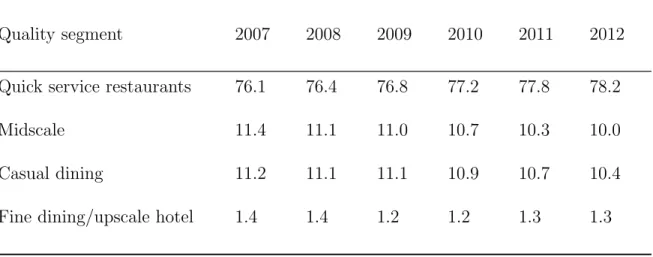
In this subsection, we discuss results obtained using data on the evolution of market shares in restaurants of different quality levels. This data set collected by the NPD Group (a marketing consulting firm) includes restaurant traffic (number of meals served) and consumer spending in restaurants broken into four categories of service: quick-service restaurants, midscale restaurants, casual dining, and fine dining/upscale hotel. These categories are designed to represent different levels of quality.
These data can shed light on the appropriateness of our assumption that the price of a good or service is a good proxy for its quality. If we sort firms using the average price of a meal as a proxy for quality, we obtain a sorting by quality tiers similar to NPD’s.14 The average price of dinner (lunch) is $6.5 ($5.8) in quick-service restaurants,
14There is a literature on the role of search frictions in generating price dispersion. While search
frictions are clearly important, the price differences across categories in our dataset are clearly too large to be accounted for by these frictions alone. Aguiar and Hurst (2006) estimate that doubling of
$11.2 ($9.2) in midscale restaurants, and $14.9 ($11.7) in casual dining.15
We find clear evidence of trading down in the NPD data. Consider first the number of meals served. Table 5 shows that the percentage of meals served by quick-service restaurants increased from 76.1 percent in 2007 to 78.2 percent in 2012. At the same time, the fraction of meals served declined in all the other segments: midscale, casual and fine-dining.16 Table 6 reports results for market share. We see that over the period
2007-2012 the market share of quick-service restaurants rose from 57.7 percent to 60 percent. At the same time, the market share declined in all the other segments.17
Unfortunately, we cannot do our accounting calculations directly with these data because we do not have the breakdown of labor intensities for the restaurant categories used by NPD. However, we can use the labor intensity estimates for Food services and drinking places reported in Tables 1 and 2, which are based on Yelp! data, as a proxy for the labor intensity in the NPD categories.18 To do so, we equate the low, middle and high quality categories in Yelp! to Quick Service, Mid-scale plus Casual Dining, and Fine Dining categories in NPD, respectively. We find that trading down accounts for 92 percent of the fall in employment. These results are similar to the total effect of trading down (including both trend and cycle) that we estimated using the Yelp! data (88 percent). Since we only have data from NPD since 2007, we cannot separate trend effects from cyclical effects.
shopping frequency lowers the price paid for a given good by 7 to 10 percent. The price differences across different categories in our data are almost an order of magnitude larger than these estimates.
15These price data were collected in March 2013. We do not have average meal prices for fine-dining
restaurants.
16There is also some evidence in the NDP data that consumers traded down in terms of the meal
they choose to eat at restaurants, eating out at breakfast and lunch instead of at dinner.
17Tables 5 and 6 show that after the worst of the recession was over in 2010, fine dining started to
recover. But overall, the fraction of meals served and market share of fine dining are still lower in 2012 than in 2007.
18NPD provided us with a partial list of restaurants classified according to the NPD categories.
Using this list, we concluded that their classification is almost identical to the one we obtain using Yelp!
Table 5: Percentages of Restaurant Traffic by Year and Quality Segment
Quality segment 2007 2008 2009 2010 2011 2012 Quick service restaurants 76.1 76.4 76.8 77.2 77.8 78.2
Midscale 11.4 11.1 11.0 10.7 10.3 10.0
Casual dining 11.2 11.1 11.1 10.9 10.7 10.4
Fine dining/upscale hotel 1.4 1.4 1.2 1.2 1.3 1.3 Note: The data is from NPD Group.
Table 6: Restaurant Market Share by Year and Quality Segment
Quality segment 2007 2008 2009 2010 2011 2012 Quick service restaurants 57.7 58.0 58.7 59.0 59.4 60.0
Midscale 15.4 15.2 15.1 14.8 14.5 14.1
Casual dining 21.5 21.4 21.4 21.3 20.9 20.5
Fine dining/upscale hotel 5.5 5.3 4.9 5.0 5.2 5.4 Note: The data is from NPD Group.
2.5
Substitution across categories
In our analysis, we focus on the implications of trading down for employment. We also studied the employment implications of substitution across categories, for example from luxuries to necessities. Our analysis is based on CEX and NIPA PCE data (see Appendix C for more detail on the calculations).
It is well known that different categories of expenditure have different income elas-ticities. As a result they differ in their cyclical properties. For example, expenditure on food away from home falls during recessions by much more than expenditures on personal care.
We find that substitution across categories has a negligible effect on employment. This result is driven by the low correlation between income elasticities of different categories and labor intensity is quite low. For example, both food away from home and vehicle purchases fall during recessions. But food away from home has high labor intensity, while vehicle purchases has low labor intensity. We summarize our results in Appendix C.
3
Quality choice in business-cycle models
In this section, we use several business-cycle models to show that the presence of quality choice amplifies the response shocks. We first derive some theoretical results in a partial-equilibrium setting. We then study a representative-agent general-partial-equilibrium model and show that this model can help resolve some long-lasting challenges in the business-cycle literature. Finally, we extend our model to include heterogeneity in consumer quality choices. This extension allows us to draw a tighter connection between the model and our empirical work.
We focus our discussion on flexible-price version models. We show in Appendix F that the same mechanism that amplifies real shocks also amplifies nominal shocks. We do so by embedding quality choice in an model with Calvo (1983)-style sticky prices.
3.1
A partial-equilibrium model
3.1.1 Production
We begin by describing the production side of the economy, which is the same across the models we discuss. Consumer goods are produced by a continuum of measure one of competitive firms according to the following production function:
Ct=At α HC t qt ρ + (1−α) KtCρ 1ρ , (8)
where qt denotes quality and HtC and KtC denote labor and capital employed in the
consumption sector, respectively.
The consumption firms’ problem is to maximize:
maxPq,tCt−WtHtC−rtKtC. (9)
where Wt and rt denote the wage and rental rate, respectively. The solution to this
problem implies that the equilibrium price of a consumption good with quality qt is
given by Pq,t = 1 At h α1−1ρ(q tWt) ρ ρ−1 + (1−α) 1 1−ρr ρ ρ−1 t i ρ−1 ρ (10) We assume that ρ < 0, so there is less substitution between capital and labor than in a Cobb-Douglas production function. It is easy to show that this assumption is necessary so that, consistent with our empirical results, higher-quality goods are more labor intensive. The assumption that ρ < 0 also implies that the price of a consumption good is an increasing function of its quality. This property is consistent with our empirical approach which used price as a proxy for quality.
The optimal factor intensity given by HC t KC t =q ρ ρ−1 t α 1−α rt Wt 1−1ρ . (11)
Since ρ < 0, a fall in the quality chosen by household reduces, ceteris paribus, the demand for hours worked. This effect amplifies the response of the economy to shocks.
3.1.2 Household
On the household side we consider two different models. The utility function is non-homothetic in consumption in both models. As we discuss below, this condition is necessary in order for the optimal level of quality chosen by the household to be an increasing function of income. We first consider a model in which households choose the quality of the single good they consume. We then consider a model in which households consume two goods with different levels of quality.
Variable quality model The household derives utility (U) from both the quantity
(C) and quality (q) of consumption and solves the following maximization problem
maxU(Ct, qt), (12)
s.t.
Pq,tCt=ξt, (13)
where ξ is the household’s income. The first-order conditions for consumption and quality imply that:
U2(Ct, qt) U1(Ct, qt) = P 0 q,tCt Pq,t , (14) We assume that U1(C, q)>0, U2(C, q)>0. (15)
The requirement that quality be a normal good, so that higher-income consumers choose to consume higher-quality goods, imposes restrictions on the utility function. The above equations imply that if U is homogeneous in C, quality is independent of income. So, in order for quality to be a normal good,U must be non-homothetic inC.
With this requirement in mind, we adopt the following parametric form of the utility function
U(Ct, qt) =
qt1−θ
We compare the response of labor demand to exogenous changes in household in-come, for constant values ofW andrin versions of the model with and without quality choice.19 In the model without quality choice, q is not time varying and the household budget constraint is simplyCt=ξt. The following proposition, proved in Appendix H,
summarizes the key result.
Proposition 1. For given levels ofWandr, the fall in hours worked employed by firms
in response to an exogenous fall in household income is always higher in the model with quality choice.
The intuition for this result is as follows. Consider first the model without quality choice. A drop in household income leads to a reduction in the quantity of consumption goods demanded. Since the prices of the two production factors are constant, the firm reduces the demand for labor and capital in the same proportion (see equation (11) with a constant value of q). Consider now the model with quality choice. A fall in consumer income is associated with a fall in the quantity and quality consumed. The fall in quality leads firms to contract more the demand for labor than the demand for capital (again, see equation (11) ). As a result, hours worked fall more in the economy with quality choice.
Stone-Geary model In this model households consume two goods with different
levels of quality. These goods enter the utility function according to a Stone-Geary utility function:20
M axC1,C2σ1log(C1−φ1) +σ2log(C2) (17)
19In the model with quality choice, the price of consumption changes in respond to changes in the
optimal quality chosen by the household.
20This form of utility is widely used in the literature on structural change, see e.g. Echevarria (1997),
subject to
2 X
j=1
PjCj =ξt. (18)
Good 1 is an inferior good in the sense that its demand income elasticity is lower than one. Good 2 is a superior good in the sense that its demand income elasticity exceeds one. Since we want quality consumed to be an increasing function of income, we assume thatq2 > q1. Both consumption goods are produced according to
Yj =Cj =A α Hj qj ρ + (1−α) (Kj) ρ 1ρ . (19) It is easy to show that the expenditure share of good 2 is given by
sC2 = σ2 σ1+σ2 1− P1φ1 ξt , (20)
while the expenditure share of good 1 is given by sC1 = σ1 σ1+σ2 + σ2 σ1+σ2 P1φ1 ξt . (21)
The following proposition, proved in Appendix H, summarizes this model’s key property
Proposition 2. For given levels of W and r, the fall in hours worked employed by firms
in response to an exogenous fall in household income is always higher when the superior good is more labor intensive than the inferior good.
The intuition for this result is simple. The share of the inferior good increases in response to a negative income shock. If this sector has a lower labor intensity than the superior good, then as its share increases, reducing the demand for labor above and beyond the direct impact from the fall in income.
3.2
A general-equilibrium model
In this section, we solve a general equilibrium version of the model with variable quality discussed above.21 Our goal is to assess the qualitative and quantitative implications of
21We focus on the variable-quality the model because, for the parameters we consider, it performs
quality choice when prices of goods and factors of production are endogenous. We first study the properties of a representative-agent version of the model. Then we discuss the properties of an heterogenous-agent version of the model. The household chooses quantity consumed, quality consumed and hours worked to maximize
maxE0 ∞ X t=0 βt " qt1−θ 1−θ log(Ct)−φ Hs,t1+ν 1 +ν # , (22) subject to Pq,tCt+It =WtHt+rtKt, (23) Kt+1 =It+ (1−δ)Kt, (24)
where E0 is the conditional expectation operator. As above, Wt is the wage rate, rt is
the rental rate of capital, andPq,t is the price of one unit of consumption with quality
q. It denotes the level of investment.
We assume that the disutility of work is separable from the utility of consumption. An advantage of this functional form is that it nests the usual separable logarithmic utility in consumption and power disutility in hours worked as a special case. This property simplifies the comparison of versions of the model with and without quality choice.
Consumption goods are produced by a continuum of measure one of competitive firms with the following production function
Ct=At α HtC qt ρ + (1−α) KtCρ 1ρ . (25)
Investment goods are produced by a continuum of measure one of competitive firms with the following production function
It =At α HtI qI ρ + (1−α) KtIρ ρ1 . (26)
Since our evidence about trading down is only for consumption goods, we assume that investment goods have a constant quality level,qI. We set this investment quality
level equal to the steady state level of quality in the consumption goods sector. This assumption ensures that differences in the steady-state levels of labor intensity in the consumption and investment sectors play no role in our results.
We choose the investment good as the numeraire, so its price is equal to one. The problem of a producer of investment goods is
maxIt−WtHtI −rtKtI. (27)
whereHI
t and KtI denote labor and capital employed in the investment sector,
respec-tively.
This investment production function is the same as the one used in the consumption sector but the level of quality is constant.
First-order conditions The first-order conditions for the household problem are as
follows. The first-order condition forCt is:
qt1−θ 1−θ
1 Pq,tCt
=λt, (28)
whereλt denotes the Lagrange multiplier associated with the budget constraint of the
household in period t.
The first-order conditions for qt is:
qt−θlog(Ct) = λtCtPq,t0 . (29)
Combining the last two equations, we see that the quantity consumed comoves with the elasticity of the price with respect to quality,
log(Ct) = 1 1−θ Pq,t0 qt Pq,t . (30)
The first-order conditions for hours worked and capital accumulation have the fol-lowing familiar form
χHs,tν =λtWt, (31)
λt=βEtλt+1(1−δ+rt+1) , (32)
Equilibrium The equilibrium definition is as follows. Households maximize utility
taking the wage rate, the rental rate of capital, and the price-quality schedule as given. Since households are identical, they all choose the same level of quality and only this quality level is produced in equilibrium. Firms maximize profits taking the wage rate and the rental rate of capital as given. The labor and capital market clear, so total demand for labor and capital equals their supply:
KtC +KtI = Kt, (33)
HtC+HtI = Hs,t. (34)
Real output (Yt) in the economy is given by:
Yt=Pq,tCt+It. (35)
This expression assumes that real output is computed using hedonic adjustments: when the price of consumption rises, the statistical authorities recognize that this rise is solely due to an increase in the quality of the goods consumed.
Simulation We solve the model numerically by linearizing the equilibrium conditions
around the steady state and using the parameters described in Table 7. There are three parameters that cannot be directly calibrated from the existing literature: α,ρ, andθ. The first two are calibrated to match the consumption share in the economy (80%) and the labor share in income (68%). To facilitate comparison, we set these parameters to be the same in all of the models we discuss below. We evaluate the properties of the model for three different values ofθ.
Table 7: Calibration
Parameter Moment/Description Value
β Quarterly discount rate 0.985 ν Inverse of Frisch elasticity 0.001 φ Match steady state H 5.31 δ Depreciation rate 0.025 κ AR(1) coefficient of TFP 0.95 α Production function share 0.1 ρ EOS between K and N: 1−1ρ −0.5 θ Elasticity of utility to quality 0.5
To study the model’s business cycle implications, we simulate quarterly versions of the models with and without quality choice model driven by an AR(1) TFP shock. We HP-filter both the U.S. data and the time series generated by the models with a smoothing parameter of 1600.
Table 8 reports the standard deviation relative to aggregate output (denoted by σX/σGDP) and the correlation with aggregate output (denoted byCorX,GDP) with the
following variables: consumption, investment, total hours worked, hours worked in the consumption sector, hours worked in the investment sector, the labor wedge, and the marginal utility of consumption. Columns 1-2, 3-4, and 5-6 in Panel A present the results for U.S. data, our representative agent model with quality choice and the model without quality choice, respectively. This latter model is a benchmark one-sector Real Business Cycle (RBC) model with a CES production function. For future reference, columns 7-8 in Panel A present the results for the heterogeneous agent model with quality choice. Panel B displays the second-moment implications of the representative agent model for different calibrations of θ.
Table 8: Second Moments
Panel A:
Variable Data RA Quality:θ= 0.5 No Quality Het Agents with Quality
σX σGDP Cor X,GDP σX σGDP Cor X,GDP σX σGDP Cor X,GDP σX σGDP Cor X,GDP Total Hours 1.1 0.78 0.84 0.99 0.55 0.97 0.81 0.99 Hours in C 0.80 0.48 0.41 0.93 0.10 -0.76 0.19 0.80 Hours in I 2.48 0.86 2.86 0.94 3.17 0.95 2.64 0.96 Consumption 0.80 0.85 0.56 0.93 0.42 0.90 0.40 0.883 Investment 3.16 0.87 3.05 0.95 3.59 0.98 2.88 0.99 Labor Wedge 1.1 -0.69 0.40 -0.98 NA NA NA NA λ NA NA 0.18 -0.71 0.42 -0.90 NA NA Panel B:
Variable RA with Quality:θ= 0.33 RA with Quality:θ= 0.7
σX σGDP Cor X,GDP σX σGDP Cor X,GDP σX σGDP Cor X,GDP Total Hours 0.98 0.99 0.70 0.99 Hours in C 0.60 0.48 0.23 0.95 Hours in I 4.18 0.86 2.72 0.95 Consumption 0.60 0.85 0.53 0.95 Investment 4.21 0.87 3.05 0.97 Labor Wedge 0.53 -0.73 0.21 -0.95 λ 0.14 0.29 0.33 -0.88 Amplification
Consider first Panel A. This panel shows that the volatility of hours is higher in the version of the model with quality choice. This amplification is visible in Figure 1. This figure shows the impulse response of labor and output to the same negative TFP shock
in the model with and without quality choice.
Figure 1: Impulse response of hours and output for a fall inA (% deviations from the steady state)
The interaction between the endogeneity of the labor supply and the choice of quality gives rise to an additional source of amplification: income effects on the labor supply are much weaker in the model with quality choice than in the model with no quality choice. The intuition for this property is as follows. In the model without quality choice, agents have only one margin to adjust their consumption in response to an exogenous income shock, which is to reduce the quantity they consume. In the model with quality choice agents can use two margins of adjustment: change the quantity and the quality of their consume. As a result, the marginal utility of consumption, λ, responds less to an income shock in the version of the model with quality choice. In our calibrated model, the volatility of λt is 33 percent lower in the model with quality choice (see
Table 8). These weaker income effects lead to larger movements in hours worked (see equation (31)). Panel B shows that the magnitude of amplification depends on the value ofθ, the parameter that controls the curvature of the utility from quality. Lower values of θ imply that quality is more volatile and hence that the quality channel is more quantitatively significant, providing more amplification.
Comovement
The results reported in Table 8 show another interesting difference between the models with and without quality choice. As emphasized by Christiano and Fitzgerald (1998), hours worked in the consumption sector are procyclical in the data but coun-tercyclical in the standard RBC model.22 The model with quality choice generates
procyclical hours worked in the consumption sector.
To understand this property, it is useful to write the first-order condition for labor choice for a standard RBC model with a Cobb-Douglas production function:
φ HtC+HtIν = α HC
t
. It is clear that HI
t and HtC are negatively correlated, so that HtI and HtC cannot be
both positively correlated with aggregate output. Using a CES production function changes the form of the first-order condition but does not help generate comovement.
Consider the first-order condition for labor choice in the model with quality choice: φ HtC +HtIν = q 1−θ−ρ t 1−θ α (HC t ) 1−ρ At Ct ρ . This equation shows that HC
t and HtI can be positively correlated, because quality is
procyclical. The rise (fall) in quality increases (decreases) the demand for labor in the consumption sector, contributing to the comovement between HtC and HtI.
22To classify the sectors into “consumption” and “investment” we follow standard practice. We use
the BEA’s 2002 benchmark I/O “use tables.” To compute the share of sectoral output used for private consumption vs. private investment, we assign a sector to the consumption (investment) sector if most of its final output is used for consumption (investment). For the hours/sectors data we use the Current Employment Statistics 1964:Q1 - 2012:Q4.
An endogenous labor wedge Shimer (2009) modifies the standard Euler equation for labor to allow for a “labor wedge,”τt, that acts like a tax on the labor supply:
φHtν = (1−τt)
1 Ct
wt. (36)
He then computes the labor wedge, using empirical measures ofHt,Ct, andwt. Shimer
(2009) finds thatτtis volatile and counter-cyclical: workers behave as if they face higher
taxes on labor income in recessions than in expansions. The analogue of equation (36) in our model is
φHtν = q 1−θ t 1−θ 1 Ct wt Pq,t . (37)
Since the quality consumed, qt, is procyclical (see Table 8), our model generates a
counter-cyclical labor wedge.
Summary We find that introducing quality choice into an otherwise standard model
amplifies the response to real shocks, giving rise to higher fluctuations in hours worked. This property enables the model to match the overall relative variability of hours to output that is observed in U.S. data. Moreover, the model can also account for the sectoral comovement in hours worked in the consumption and investment sectors and generate a counter-cyclical labor wedge.
3.3
An heterogenous-agent model
In the representative-agent version of the variable-quality model there’s a single level of quality consumed in equilibrium. In this subsection, we consider an extension of the model in which there are multiple quality levels produced in equilibrium. This distribution of quality facilitates the comparison of the model implications and our empirical findings. We show that the key properties of the representative-agent model are preserved in the presence of heterogeneity.
We assume that individuals are endowed with different levels of efficiency units of labor, , distributed according to the cdf Γ(). To reduce the dimension of the state space and make the problem more tractable, we model household decisions as made by families that contain a representative sample of the skill distribution in the economy.
The family’s objective is to maximize V =M ax{C,t,q,t,Hs,,t,Ks,,t+1,I,t} ∞ X t=0 βt ˆ ω ( q,t1−θ 1−θ log(Cq,t)−φ Hs,,t1+ν 1 +ν ) Γ0()d. (38) The variableωdenotes the weight attached by the family to an individual of ability
. The variables q,t, Cq,t, and Hs,,t denote the quality and quantity of the good
consumed and the labor supplied by an individual with abilityin periodt, respectively. The family’s budget constraint is:
Kt+1 = ˆ WtH,t−Pq,tCq,t Γ0()d+rtKt+ (1−δ)Kt, (39)
where Pq,t is the price of one unit of consumption of the quality consumed by an
individual with ability in period t. The variable Kt denotes the family’s stock of
capital.
The first-order conditions for the quantity and quality of consumption and hours worked for each family member are the same as in the representative-agent model (equations (28)-(30)).
The goods consumed by agents with abilityare produced by perfectly competitive producers according to the following CES production function:
Y,t =At α Hd,,t q,t ρ + (1−α) (Kd,,t)ρ 1ρ , (40)
The variables Hd,,t and Kd,,t denote the labor and capital employed by the producer,
respectively. As in our representative-agent model, we assume thatρ <0.
The problem of a producer who sells its goods to consumers with ability is given by
This solution to this problem implies that the price schedule, Pq,t, is Pq,t = 1 At h α1−1ρ(q ,tWt) ρ ρ−1 + (1−α) 1 1−ρr ρ ρ−1 t iρ −1 ρ , (42)
and that firm’s optimal labor-capital ratio is Hd,,t Kd,,t =q ρ ρ−1 ,t α 1−α rt Wt 1−1ρ . (43)
Investment goods are produced by a continuum of measure one of competitive firms according to: It=At α Hd,inv,t qinv ρ + (1−α)Kd,inv,tρ 1ρ , (44)
whereHd,inv,t and Kd,inv,t denote labor and capital employed in the investment sector,
respectively. As in the representative-agent model, we assume that there is no quality choice in the investment sector.
Equilibrium The equilibrium definition is as follows. Households maximize utility
taking the wage rate per efficiency unit of labor, the rental rate of capital, and the price-quality schedule as given. Firms maximize profits taking the wage rate per efficiency unit of labor and the rental rate of capital as given. The labor market clears, so total demand for labor equals total supply:
ˆ Hd,,td+Hd,inv,t= ˆ Hs,,tΓ0()d(). (45)
The capital market clears, so total demand for capital equals total supply: ˆ
Kd,,td+Kd,inv,t=Kt. (46)
The goods market clear so, for each quality level, production equals consumption: Y,t = Γ0()Cq.t. (47)
Using investment as the numeraire, real output,Yt, is given by:
Yt=It+
ˆ
3.3.1 Calibration
Diamond and Saez (2011) argue that U.S. income follows approximately a Pareto dis-tribution. For this reason, we assume that ability follows a Pareto disdis-tribution.
To solve the model numerically, we discretize the Pareto distribution using a support withn ability levels. The value of n needs to be large enough so that there are enough agents near the lower bounds of the high and medium quality bins. It is the trading down by these agents in response to a negative shock that leads to changes the market shares of the three quality categories. At the same time, since we solve for the optimal quality and quantity of the consumption good for each ability, we are limited in the number of types we can consider. We discretize the support of the distribution with n= 100 grid points.
We set the shape parameter of the Pareto distribution to 1.5, which is the value estimated by Diamond and Saez (2011). The ratio of the upper and lower bound of the support of thedistribution, max/min, is chosen to match the income ratio of the top
5 percent to the second income quintile between 2010-2014. This ratio is equal to 4.9.23
We choose the weights attached by the family to a worker of skill to be the ratio of to the average skill, /E().
For comparability, we setρ,α to be equal to the values reported in Table 7. We find that the resulting consumption share and labor share in this economy are close to those in the representative agent (75% and 61% respectively). As in the representative agent model, we assume that the quality parameter in the investment production function is constant. One of our calibration targets is to equate the quality parameter in the investment sector with the revenue weighted quality values in the consumption sector in the steady state.24
Interestingly, while not being a target, the labor intensities in the model come quite
23See the data in
http://www.taxpolicycenter.org/statistics/historical-income-distribution-all-households
close to their empirical counterparts. Specifically, we calculate the log of the ratio of the labor intensity in the “middle quality” market to the labor intensity in the “low quality” market in 2007, and the log of the ratio of the labor intensity in the “high quality” market to the labor intensity in the “middle quality” market in 2007. These values are 0.31 and 0.16 in the model while in the data we found them to be 0.38 and 0.16. We discuss the details of this calculation in Appendix G.
3.4
Results
Steady State Figure 2 illustrates some key properties of the steady state that are
consistent with our empirical facts. The first panel shows that higher-skilled individuals (those with a higher ) consume more quantity and higher quality. The second panel shows that higher quality goods have higher prices and are produced with higher labor intensities.
The Effect of Trading Down Recall that around half of the observed fall in
em-ployment was due to cyclical trading down. We follow the empirical approach described in Section 2, summarized in equations (4)-(6), to compute the impact of trading down on employment in our model.
We subject the economy to a TFP shock that generates the same 7 percent increase in the share of the low-quality segment we estimate with Yelp! data. We then calculate the market share of the low, middle and high qualities markets, and the labor intensity in each of these three segments in the period when the shock occurs. We then use this information to compute the counterfactual change in hours worked that would have occurred in the absence of trading down.
Overall, we find that hours worked in the consumption sector fall on impact by 4.8 percent. We find that, absent trading down, hours worked would have fallen by only 2.7 percent. These results imply that trading down accounts for around 43 percent of the observed changes in employment, which is roughly consistent with our empirical
estimates.
Figure 2: Optimal Choices and Implications
Business Cycle Moments The last two columns in Panel A in Table 8 reports the
cyclical properties of the heterogeneous agent model. We see that the business-cycle properties of this model are very similar to those of the representative agent model. The heterogeneous-agent model generates amplification in hours worked, comovements of hours worked in the consumption and investment sectors, and a countercyclical labor wedge.
4
Conclusion
We document two facts. First, during the Great Recession consumers traded down in the quality of the goods and services they consumed. Second, lower quality prod-ucts are generally less labor intensive, so trading down reduces the demand for labor. Our calculations suggest that trading down accounts for about half of the decline in employment during the Great Recession.
We study a general equilibrium model in which consumers choose both the quantity and quality of consumption. We show that in response to a fall in TFP the model gen-erates trading down in quality and declines in employment that are broadly consistent with our empirical findings.
The presence of quality choice improves the performance of the model along two dimensions. First, cyclical changes in the quality of what is consumed amplifies the effects of shocks to the economy, resulting in higher variability in hours worked. Sec-ond, the model generates comovement between labor employed in the consumption and investment good sectors.
5
References
Aguiar, Mark and Erik Hurst “Lifecycle production and prices,” The American Economic Review, 97(5): 1533-59, 2007.
Aguiar, Mark, Erik Hurst and Loukas Karabarbounis “Time use during the Great Recession,” The American Economic Review: 1664-1694, 2013.
Anderson, Eric, Sergio Rebelo and Arlene Wong “On the cyclicality of markups,” manuscript, Kellogg School of Management, Northwestern University, 2017.
Burns, Arthur and Wesley MitchellMeasuring business cycles, New York, National Bureau of Economic Research, 1946.
Burstein, Ariel, Eichenbaum, Martin, and Sergio Rebelo, 2005. “Large devaluations and the real exchange rate.”Journal of Political Economy 113 (4), 742–784.
Chen, Natalie and Luciana Juvenal “Quality and the great trade collapse,” manuscript, International Monetary Fund, 2016.
Coibion, Olivier, Yuriy Gorodnichenko and Gee Hee Hong “The Cyclicality of sales, regular and effective prices: business cycle and policy implications” The American Economic Review, 105, 993-1029, 2015.
Diamond, Peter, and Emmanuel Saez, 2011. “The case for a progressive tax: from basic research to policy recommendations”The Journal of Economic Perspectives, 165-190.
Echevarria, Cristina, “Changing Sectoral Composition Associated with Economic Growth”International Economic Review, 38, 431-452, 1997.
Gilchrist, Simon, Jae Sim, Egon Zakrajsek, and Raphael Schoenle “Inflation dy-namics during the financial crisis,” manuscript, 2015.
Gorodnichenko, Yuriy and Michael Weber “Are sticky prices costly? Evidence from the stock market,” manuscript, University of California, Berkeley, 2015.
Struc-tural Transformation” in Handbook of Economic Growth, vol. 2 edited by Philippe Aghion and Steven N. Durlauf, pages 855-941, 2014.
Kaplan, Greg and Guido Menzio “Shopping externalities and self-fulfilling unem-ployment fluctuations,” Journal of Political Economy, 124(3), 2016.
Kongsamut, Piyabha , Sergio Rebelo, Danyang Xie; “Beyond Balanced Growth,” The Review of Economic Studies, Volume 68, Issue 4, 1 October 2001, Pages 869?882,
Nevo, Aviv and Arlene Wong “The elasticity of substitution between time and mar-ket goods: Evidence from the Great Recession,” manuscript, Northwestern University, 2015.
Weber, Michael “Nominal rigidities and asset pricing,” manuscript, University of Chicago, 2015.
Appendix
In this appendix, we accomplish four main tasks. First, we provide more details about the construction of the Yelp! and PPI data set. Second, we report additional robustness checks on the estimates presented in the main text regarding the effects of trading down on employment. Third, we discuss the algorithm used to calibrate the heterogeneous-agent model. Finally, we discuss a version of the representative model with Calvo-style price stickiness.
A
Yelp! data
We scraped data for Yelp in April 2014. For firms that own more than one brand, we compute the average price category for each brand and then compute the average price category for the firm, weighting each brand by their sales volume. One concern about this procedure is that we might be averaging high-quality and low-quality brands. In practice, this situation is rare: 73 percent of the firms in our sample have a single brand. For multi-brand firms, 54 percent have all their brand in the same price category. For example, the firm Yum! Brands owns three brands (Taco Bell, KFC, and Pizza Hut), but they are all in the same price category (low price). For robustness, we redid our analysis including only firms that either have a single brand or have all their brands in the same price category. We obtain results that are very similar to those we obtain for the whole universe of firms.
In merging the data with Compustat we note that for companies with operations outside of the U.S., we use the information on sales by business region to compute U.S. sales. We also use the break down of employment by business region to compute labor intensity in the U.S. We exclude from our sample manufacturing firms for which this breakdown is not available. For retail firms, foreign operations are generally small, so we include companies with foreign operations in our sample. As we robustness check, we redo our analysis excluding these companies. The results are similar to those we
obtain for the full sample.
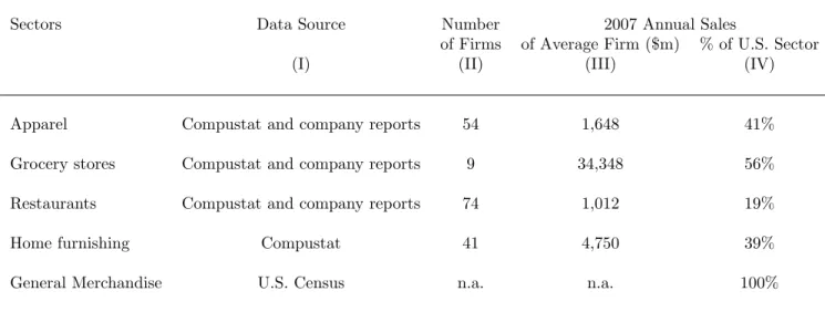
Table 9 presents some description of the data used to analyze quality shifts in expenditure in five retail sectors. It describes the data source (column I), the number of firms covered in the sample in 2007 (II), the average annual firm sales revenue (III), and the percent of the overall sector sales that our sample covers (IV).
Table 9: Data Sample Description
Sectors Data Source Number 2007 Annual Sales
of Firms of Average Firm ($m) % of U.S. Sector
(I) (II) (III) (IV)
Apparel Compustat and company reports 54 1,648 41% Grocery stores Compustat and company reports 9 34,348 56% Restaurants Compustat and company reports 74 1,012 19%
Home furnishing Compustat 41 4,750 39%
General Merchandise U.S. Census n.a. n.a. 100%
Note: This table describes for each sector the data source used (I), the number of firms within the sample (II), and the average annual sales of each firm (III). (IV) reports the share of the sales of the entire sector that our data set covers.
B
PPI
Using the PPI data presents two challenges. First, firms in the same industry re-port prices that correspond to different units of measurement, e.g. some firms rere-port price per pound, others price per dozen. To circumvent this problem, we first convert prices into a common metric whenever possible (for example, converting ounces to into pounds). We then compute the modal unit of measurement for each 6-digit NAICS
category and restrict the sample to the firms that report prices for this model unit. This filtering procedure preserves 2/3 of the original data, which is comprised of 16,491 establishments out of a sample of about 25,000 establishment surveyed by the PPI. Some establishments are excluded because we only include items that are recorded at the modal unit of measure within the 6-digit product category.
Second, some of the firms included in the PPI data offshore their production, so their reported employment does not generally include production workers. It includes primarily head-office workers and sales force in the U.S. Using information in the firms’ annual reports, we exclude firms that have most of their production offshore. The resulting data set preserves over half of the merged PPI/Compustat data.
In order to construct a quality measure for each firm, we proceed as follows. For each product k that establishment esells in year t, we calculate its price, pket, relative
to the median price in the industry for product k in year t, ¯pkt:
Rket =pket/p¯kt.
Our analysis is based on products defined at a six-digit industry code level and then further disaggregated by product type. Therefore, although the results are presented at a 2-digit level, all relative prices are defined at a narrow 6-digit level for comparability. For details of this disaggregation, see Table 11 of the BLS PPI Detailed Report. The variable ¯pkt is a shipment-value weighted average within the product category. For
reporting purposes, we aggregate the results to the two-digit level. The aggregation is based on shipment revenue.
For single-product establishments, we use this relative price as the measure of the quality of the product produced by establishmente. For multi-product establishments, we compute the establishment’s relative price as a weighted average of the relative price
of different products, weighted by shipment revenue in the base year (wke):25
Ret =
X
k∈Ω
wkeRket.
where Ω denotes the set of all products in the PPI data set that we examined.
C
Substitution across categories
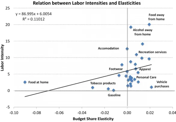
Our main analysis focuses on trading-down behavior within categories. We also exam-ined substitution across consumption categories and the effect on employment. We use data from the CEX Survey and NIPA personal consumption expenditures (PCE). We consider 31 different consumption categories (see Figure 3).
We examine the effect of across-category substitution on employment in two steps. First, we construct the labor intensity for each consumption category. We match CEX consumption categories with the NIPA PCE commodity definitions.26 This allows us
to the Input/Output commodity-level data to construct labor intensity measures for each consumption category. Second, we compute the change in budget share for each consumption category over 2007-2012 for the average household. To isolate out the cyclical component of the budget reallocation across consumption categories, we esti-mate elasticities of the category budget shares to total household expenditure. We then multiply the elasticities by the actual change in household expenditure to obtain the change in budget allocation for each category.
We derive shifts in expenditure associated with the recessionary drop in household income by estimating the following Engel curve elasticities:
whtk =αk+βkln(Xht) +
X
j
γjln(Pjt) +θkht·Zht+kht, (49) 25This approach for constructing firm-level price indices is similar to that used by Gorodnichenko
and Weber (2014), and Gilchrist et al (2014). However, we compute relative prices using a much finer product definition than these authors. We refer the reader to Section II in Gorodnichenko and Weber (2014) for a discussion of how the BLS samples products and firms.
wherewk
ht is the budget share allocated to category k by household h at timet; Xht is
total household expenditure; and Pjt is the price index of each expenditure category j
at time t. The variable Zht is a vector of household demographics variables, including
the age and square of the age of the head of household, dummies based on the number of earners (<2,2+), and household size (<2,3-4,5+). The error term is denoted by k
ht. We estimate equation (49) using household sample weights given in the CEX data
based on the 1980-2012 waves of the CE Surveys. The coefficient βk gives the fraction
change in budget share allocation to expenditure category k, given a 100 percentage point change in total household expenditure.27
27There potential issues that arise in estimating equation (49). For instance, mismeasurement of
in-dividual goods may be cumulated into total expenditure, which would bias the estimated coefficients. Aguiar and Bils (2013) for a more detailed discussion of these measurement issues associated with using the CE Survey to estimate elasticities. Therefore for robustness, we also use the standard ap-proach of instrumenting total expenditure with total income reported by the household. The estimated elasticities yield similar results to our base estimation without instrumenting.
Figure 3: Scatter plot of labor intensity and elasticities across sectors Vehicle purchases Personal Care Food at home Apparel Footwear Gasoline Tobacco products Recreation services Alcohol away from home Food away from home Accomodation y = 86.995x + 6.0054 R² = 0.11012 -5 0 5 10 15 20 25 -0.10 -0.08 -0.06 -0.04 -0.02 0.00 0.02 0.04 La bo r I nt en si ty
Budget Share Elasticity
Relation between Labor Intensities and Elasticities
Figure 3 shows there is a low positive relation between a category expenditure elasticity and its labor intensity measure. To examine the effect of across-category substitution on employment, we perform a similar exercise as our trading-down cal-culation. We compute the change in the number of employed workers between 2007 and 2012 due to changes in the shares of the expenditures categories, holding fixed the measured labor intensity.28 This exercise yields a negligible effect of the substitution
across categories on aggregate employment, in contrast to our findings of large effects of quality trading-down within categories.
28We also did the computation using actual observed change in expenditure allocations in the NIPA