Gleason Grading of Prostate Tumours with Max-Margin Conditional Random Fields

Gleason Grading of Prostate Tumours with

Max-Margin Conditional Random Fields

Joseph G. Jacobs, Eleftheria Panagiotaki, Daniel C. Alexander Centre for Medical Image Computing, Department of Computer Science,

University College London, UK [email protected]

Abstract. Prostate cancer diagnosis involves the highly subjective and time-consuming Gleason grading process. This paper proposes the use of Max-Margin Conditional Random Fields (CRFs) towards the aim of creating an automatic computer-aided diagnosis system. Unlike previous methods, this approach enables us to fuse information from multiple clas-sifiers while leveraging CRFs to model spatial dependencies. We perform grading on superpixels which reduce redundancy and the size of data. Probabilistic outputs from independent classifiers are passed as input to a Max-Margin CRF, which then performs structured prediction on the biopsy core, segmenting the image into regions of benign tissue, Gleason grade 3 adenocarcinoma and Gleason grade 4 adenocarcinoma. The sys-tem achieves an accuracy of 83.0% with accuracies of 83.6%, 86.9% and 77.1% reported for benign, grade 3 and grade 4 classes respectively.

1

Introduction

Gleason grading prostate tumour biopsies is a vital part of the prostate can-cer diagnostic process. A histopathologist performing Gleason grading first mi-croscopically examines a hematoxylin and eosin (H&E) stained biopsy core at low magnification to indentify regions of interest (ROIs) before inspecting each ROI at a higher magnification to assign it a Gleason grade. Despite being the predominant prostate tumour grading system for nearly 50 years, the Gleason system has its shortcomings. For instance, the method is very subjective with a high degree of intra- and inter-observer variability[9]. Gleason grading is also an incredibly time-consuming process. Considering approximately 60-70% of biop-sies are benign, this suggests most of a histopathologist’s time is spent sifting through benign tissue[3]. Consequently, there is a need for computer-aided diag-nosis (CAD) to improve the accuracy and efficiency of the grading process.

A significant body of research has been dedicated towards this task. Monaco et al.[8] use a probabilistic Markov Random Field (MRF) prior called a Proba-bilistic Pairwise Markov Model (PPMM) in a gland segmentation framework to enforce spatial dependencies during classification. Doyle et al.[3] and Gorelick et al.[5] both employ AdaBoost to learn meta-classifiers that aggregate

informa-Table 1: Overview of the proposed method in comparison to closely related work Method Classification Algorithm Meta-classification Spatial De-pendencies Task Doyle et al.[3]

AdaBoost Yes No Segment an image into benign and cancerous regions

Gorelick et al.[5]

AdaBoost Yes No Grade images of manually identi-fied ROIs

Monaco et al.[8]

PPMM No Yes Segment and classify glands as benign or cancerous

Proposed method

Max-Margin CRF

Yes Yes Segment an image into benign, Gleason 3 and Gleason 4 regions

tion from multiple weak ‘i.i.d. classifiers’1to produce a strong classifier. [3] uses AdaBoost in a multi-resolution pixel-wise framework to segment an image into benign and cancerous regions. On the other hand, [5] uses AdaBoost to (i) clas-sify superpixels as one of nine tissue components and (ii) grade an image based on the distribution of tissue components. Besides these, most studies focus on feature selection, using i.i.d. classifiers such as Support Vector Machines (SVMs) andk-Nearest Neighbours (k-NN) with some combination of colour, texture and morphometric features to segment or classify images[14, 11].

This paper presents a method that segments H&E stained biopsy cores into regions of benign tissue, Gleason grade 3 adenocarcinoma and Gleason grade 4 adenocarcinoma. Table 1 compares the proposed method to the closest in previous literature. We use Max-Margin Conditional Random Fields (CRFs) to perform multi-class meta-classification on the outputs of two multi-class i.i.d. classifiers while incorporating spatial dependencies into the process. Like [3] we perform classification on every region in an image (i.e. not just on segmented glands), enabling the algorithm to function even in highly cancerous regions which often have poorly defined glands[4]. However, we use superpixels to over-segment an image prior to performing classification. This significantly reduces redundancy and the size of data.

2

Proposed Method

Our solution uses machine learning and computer vision algorithms to segment and grade H&E stained biopsy cores. The method employs Simple Linear Iter-ative Clustering (SLIC)[1] to over-segment an image into superpixels. We then extract colour and texture features from each superpixel to perform classification in two stages. In the first stage, we use ak-NN and an SVM to obtain individ-ual class probabilities for each superpixel. A Max-Margin CRF then acts as a meta-classifier, combining information from the first stage classifiers while

incor-1

We define an ‘i.i.d. classifier’ as a classifier that assumes data points are independent and identically distributed (the i.i.d. assumption).

Fig. 1: Overview of the proposed method.

porating spatial dependencies into the prediction process. The following sections describe and motivate the selection of each individual algorithm in more detail.

2.1 Pre-processing

The computational complexity of performing inference on a general CRF in-creases with the number of vertices and edges in the graph. Our method groups perceptually similar pixels to form superpixels. This reduces the number of ver-tices in the CRF, thus reducing the computational complexity of inference. We use SLIC[1] to do this as the algorithm is simple, fast and memory efficient. Given a superpixel sizeS, SLIC clusters an imageI in the colour and spatial domains using an algorithm similar tok-means clustering to formk=|I|_S2 superpixels.

Next, we extract colour and texture features from each superpixel. A 17-bin histogram of RGB pixel intensities and the mean RGB pixel intensity represent the colour of a superpixel while histograms of Local Binary Patterns (LBP)[12] describe its texture. We use the ‘uniform’ variant of LBP as it is both greyscale-and rotation-invariant. For each pixel c, we construct a P-bit binary number with the indicator function I[gi ≥ gc], i = 1, . . . , P where gc is the greyscale pixel intensity of c and gi are the greyscale pixel intensities of P points at a radiusR aroundc. The LBP label for uniform patterns (i.e. there are, at most, two 0/1 transitions in theP-bit number) is the number of 1s in theP-bit number while the label for non-uniform patterns isP+1. We then construct a (P+2)-bin histogram of LBP labels to obtain a texture descriptor for each superpixel.

2.2 Classification

At this stage it is possible that some superpixels may not contain enough useful information to distinguish between the three classes. A histopathologist looking at the same region would consider the information in surrounding regions to make a decision. Structured prediction offers the ability to do this by incorpo-rating spatial dependencies between superpixels into the prediction process. We perform structured prediction with a functionf :X → Yfrom the input domain

X to a structured output domainY where fw(X) = arg max

Y∈Y

gw(X, Y), X∈ X (1)

for some cost function gw(X, Y) that describes the compatibility of structured output Y with input X as parameterised by w. In our case, the input X is

the probabilistic output from our first stage classifiers, a CRF G encodes the structure of the output and we use max-margin learning to find the optimalw.

First Stage Classifiers. The first stage classifiers are ak-NN and an SVM that output class probabilities for each superpixel. The k-NN calculates class prob-abilities for each data point as the proportion of the kclosest points belonging to each class. The SVM uses a modified version of Platt scaling[6] to provide class probabilities given the decision function outputs of a non-linear SVM. The output from this stage is a 6×1 vector of class probabilities for each superpixel.

Conditional Random Fields. The graph G = (V,E) is a pairwise CRF that models the conditional probability of a structured outputY as a combination of unary and pairwise terms. We define G such that each vertex v ∈ V represents a superpixel and edges eu,v∈ E connect two adjacent superpixelsu, v∈ V. The energy or cost of a given labellingY ∈ Y is then expressed as

E(Y) =X v∈V

U(v) + X eu,v∈E

P(u, v) (2)

where U(v) is the unary term and P(u, v) is the pairwise term. U(v) encodes the compatibility of a given labelling yv ∈Y with the inputsxv ∈X at vertex v. To use the CRF as a meta-classifier, we modelU(v) as a linear combination of the class probabilities from the first stage classifiersxv. This is written as

U(v) =hwU

yv,xvi (3) where wU

yv are the unary parameters for the class yv learnt during training. P(u, v) represents the compatibility of the labellingyu and yv for the adjacent verticesuandv. This is learnt directly during training and is written as

P(u, v) =wP_yu,yv (4) wherewP_yu,yvis the symmetric pairwise parameter for the classesyuandyvlearnt during training. Performing ‘prediction’ on the CRF amounts to performing in-ference on the graphGto find the optimal solutionY?that minimises the energy function E. The general pairwise CRF is usually a loopy graph which renders exact inference intractable. However, good approximations of the solution can be obtained using a variety of methods. Here we use Alternating Directions Dual Composition (AD3_{)[7] as it gives us better performance compared to other}

algorithms such as graph cuts.

Max-Margin Learning. Our method uses the Structured SVM (SSVM) for-mulation by Tsochantaridis et al.[15] to do max-margin learning. This formula-tion is particularly appealing as it enables the use of arbitrary loss funcformula-tions. In this case we have chosen to use per-superpixel 0-1 loss, expressed as

∆( ˆY , fw(X)) = X

v∈V

where_I[a] is an indicator function and ˆY the ground truth. The SSVM minimises the following empirical risk function to learn the optimal parametersw?_:

w?= arg min w 1 2kwk 2₊ C |N | X n∈N ∆( ˆYn, fw(Xn))−gw(Xn,Yˆn)+gw(Xn, fw(Xn)) (6) HereN is the set of ground truth images.

2.3 Experimental Setup

Our experimental setup uses open source implementations of the above meth-ods[1, 2, 10, 13, 16] to make it easily reproducible. The data set contains images of H&E stained biopsy cores collected from 122 patients. These were graded by two experienced histopathologists, each with 10 years experience in genitouri-nary pathology. We select ten biopsy cores for each of the Gleason scores 3+3, 3+4, 4+3 and 4+4, ensuring each core contains a continuous Gleason pattern at least 0.4mm in length. From these, we extract 146 images of tissue segments at 20×magnification: 90 for training and 56 for testing. We create ground truth by labelling the superpixels in these images. Where there are two or more classes of pixels within a superpixel, we select the higher Gleason grade as the label.

3

Results & Discussion

The Jaccard Index (JI) quantifies the overall performance of the method. We define it as the fraction of superpixels that are correctly labelled, expressed as

JI = | ˆ

L ∩ L|

|L ∪ L|ˆ (7)

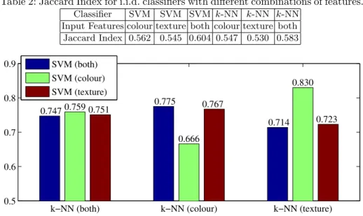
where ˆL is the set of predicted superpixel labels and L is the corresponding ground truth. We compare the performance of i.i.d. classifiers (Table 2) against our method (Figure 2), each using different combinations of normalised input features (i.e. colour/texture features only or both colour and texture features).

Table 2 shows i.i.d. classifiers struggle to perform classification at superpixel level. The two best i.i.d. classifiers are the SVM and k-NN that use both sets of features, achieving JIs of 0.604 and 0.583 respectively. In contrast, the worst variant of our method achieves a JI of 0.666. Figure 3 compares sample output from an SVM against our method, revealing its advantages over i.i.d. classifica-tion. The output of our method is a lot smoother and more consistent with the ground truth compared to the SVM. Figure 2 shows the JI of our method as we vary the input features to the first stage classifiers. When the first stagek-NN uses both sets of features, the difference in JI as we vary the features of the SVM is negligible. Similarly, there is an insignificant difference in JI when the SVM uses either texture or both sets of features. This tells us that using the best i.i.d. classifiers does not necessarily lead to better overall performance. Instead,

Table 2: Jaccard Index for i.i.d. classifiers with different combinations of features. Classifier SVM SVM SVM k-NN k-NN k-NN

Input Features colour texture both colour texture both Jaccard Index 0.562 0.545 0.604 0.547 0.530 0.583

k−NN (both) k−NN (colour) k−NN (texture)

0.5 0.6 0.7 0.8 0.9 0.7470.759 0.751 0.775 0.666 0.767 0.714 0.830 0.723 SVM (both) SVM (colour) SVM (texture)

Fig. 2: Comparison of Jaccard Indices for Max-Margin CRFs using different com-binations of input features to the first stage classifiers.

(a) Ground truth

(b) Output from a SVM (both) (c) Output from our method Fig. 3: This visualisation demonstrates the advantages of structured prediction. The output of the Max-Margin CRF is clearly a lot smoother and closer to the ground truth data than that of the SVM.

Table 3: Confusion matrix for the max-margin CRF using SVM (colour) andk -NN (texture) as input.

Predicted

Benign Grade 3 Grade 4 Total

Actual

Benign 1988 301 90 2379 Grade 3 252 2875 182 3309 Grade 4 194 370 1902 2466 Total 2434 3546 2174 8154

Table 4: Confusion matrix to evalu-ate the performance of the best clas-sifier on the separation between be-nign and cancerous regions.

Predicted Cancerous Benign Total

Actual

Cancerous 5329 446 5775 Benign 391 1988 2379 Total 5720 2434 8154

the method performs best when we use weaker first stage classifiers. The results also indicate that texture features are weighted higher than colour features in an SVM trained on both sets of features. Consequently, dropping colour features and training the SVM with texture features only has little effect on performance. We also notice the method performs best when each of the first stage classifiers use different features. We suggest that this is because each classifier provides the Max-Margin CRF with a different insight into the data.

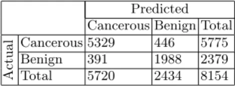
The confusion matrix of the best performing classifier for the three-class grading problem (Table 3) indicates good grading accuracy for each individual class. The method performs worst on Gleason grade 4 regions, classifying these correctly only 77.1% of the time. These regions were most often misclassified as Gleason grade 3 (15% of the time). While not ideal, this balance of classification error is preferable to the converse. This is more evident when we consider the confusion matrix for the separation between benign and cancerous regions (Table 4). The results indicate that the proposed method has a sensitivity of 92.3% and a specificity of 83.6% for separation between benign and cancerous regions. This balance of misclassification is desirable as we would rather overdiagnose than underdiagnose in a CAD system. Otherwise the system could miss cancerous regions, resulting in the disease being completely undiagnosed in some patients.

4

Conclusion & Future Work

This paper presented a novel approach to grading prostate tumour biopsies for CAD. Max-Margin CRFs were used both as a meta-algorithm and a struc-tured prediction mechanism to provide an accurate segmentation and labelling of prostate tissue images. In this case only colour and texture features were extracted from each superpixel. Using more first stage classifiers on different features (e.g. morphometric features like nuclei density) could improve the sys-tem. Specifically, we aim to capture characteristics to distinguish grade 4 from grade 3 tissue. Another weakness to address in future work is the inability to tune the trade-off between sensitivity and specificity for separation between benign and cancerous regions. We also intend to perform pixel-wise evaluation using a larger data set to enable more accurate quantification of performance.

References

1. Achanta, R., Shaji, A., Smith, K., Lucchi, A., Fua, P., S¨usstrunk, S.: SLIC Super-pixels Compared to State-of-the-Art Superpixel Methods. IEEE TPAMI 34(11), 2274–2282 (2012)

2. Chang, C.C., Lin, C.J.: LIBSVM: A library for support vector machines. ACM TIST 2(3), 27:1–27:27 (2011)

3. Doyle, S., Feldman, M.D., Tomaszewski, J., Madabhushi, A.: A Boosted Bayesian Multiresolution Classifier for Prostate Cancer Detection From Digitized Needle Biopsies. IEEE TBE 59(5), 1205–1218 (2012)

4. Epstein, J.I.: An Update of the Gleason Grading System. J Urology 183(2), 433– 440 (2010)

5. Gorelick, L., Veksler, O., Gaed, M., Gomez, J.A., Moussa, M., Bauman, G., Fenster, A., Ward, A.D.: Prostate Histopathology: Learning Tissue Component Histograms for Cancer Detection and Classification. IEEE TMI 32(10), 1804–1818 (2013) 6. Lin, H.T., Lin, C.J., Weng, R.C.: A note on Platt’s probabilistic outputs for support

vector machines. Mach Learn 68(3), 267–276 (2007)

7. Martins, A.F.T., Figueiredo, M.A.T., Aguiar, P.M.Q., Smith, N.A., Xing, E.P.: An Augmented Lagrangian Approach to Constrained MAP Inference. In: Getoor, L., Scheffer, T. (eds.) ICML 2011. pp. 169–176. Omnipress (2011)

8. Monaco, J., Tomaszewski, J., Feldman, M.D., Hagemann, I., Moradi, M., Mousavi, P., Boag, A., Davidson, C., Abolmaesumi, P., Madabhushi, A.: High-throughput detection of prostate cancer in histological sections using probabilistic pairwise Markov models. Med Image Anal 14(4), 617–629 (2010)

9. Montironi, R., Mazzuccheli, R., Scarpelli, M., Lopez-Beltran, A., Fellegara, G., Al-gaba, F.: Gleason grading of prostate cancer in needle biopsies or radical prostate-ctomy specimens: contemporary approach, current clinical significance and sources of pathology discrepancies. BJU Int 95(8), 1146–1152 (2005)

10. M¨uller, A., Behnke, S.: PyStruct-Structured Prediction in Python. JMLR 15, to appear (2014)

11. Nguyen, K., Sarkar, A., Jain, A.K.: Structure and Context in Prostatic Gland Segmentation and Classification. In: Ayache, N., Delingette, H., Golland, P., Mori, K. (eds.) MICCAI 2012, Part I. LNCS, vol. 7510, pp. 115–123. Springer, Heidelberg (2012)

12. Ojala, T., Pietik¨ainen, M., M¨aenp¨a¨a, T.: Multiresolution Gray-Scale and Rotation Invariant Texture Classification with Local Binary Patterns. IEEE TPAMI 24(7), 971–987 (2002)

13. Pedregosa, F., Varoquaux, G., Gramfort, A., Michel, V., Thirion, B., Grisel, O., Blondel, M., Prettenhofer, P., Weiss, R., Dubourg, V., VanderPlas, J., Passos, A., Cournapeau, D., Brucher, M., Perrot, M., Duchesnay, E.: scikit-learn: Machine Learning in Python. JMLR 12, 2825–2830 (2011)

14. Tabesh, A., Teverovskiy, M., Pang, H.Y., Kumar, V.P., Verbel, D., Kotsianti, A., Saidi, O.: Multifeature Prostate Cancer Diagnosis and Gleason Grading of Histo-logical Images. IEEE TMI 26(10), 1366–1378 (2007)

15. Tsochantaridis, I., Joachims, T., Hofmann, T., Altun, Y.: Large Margin Methods for Structured and Interdependent Output Variables. JMLR 6, 1453–1484 (2005) 16. van der Walt, S., Sch¨onberger, J.L., Nunez-Iglesias, J., Boulogne, F., Warner, J.D.,

Yager, N., Gouillart, E., Yu, T., the scikit-image contributors: scikit-image: image processing in Python. PeerJ 2, e453 (2014)