Investigating Key Techniques to Leverage the Functionality of Ground/Wall Penetrating Radar

(1)

University of Vermont

ScholarWorks @ UVM

Graduate College Dissertations and Theses Dissertations and Theses

2017

Investigating Key Techniques to Leverage the

Functionality of Ground/Wall Penetrating Radar

Yu Zhang

University of Vermont

Follow this and additional works at:https://scholarworks.uvm.edu/graddis Part of theElectrical and Electronics Commons

This Dissertation is brought to you for free and open access by the Dissertations and Theses at ScholarWorks @ UVM. It has been accepted for Recommended Citation

Zhang, Yu, "Investigating Key Techniques to Leverage the Functionality of Ground/Wall Penetrating Radar" (2017).Graduate College Dissertations and Theses. 799.

(2)

INVESTIGATING KEY TECHNIQUES TO LEVERAGE THE FUNCTIONALITY OF GROUND/WALL PENETRATING RADAR

A Dissertation Presented

by Yu Zhang

to

The Faculty of the Graduate College of

The University of Vermont

In Partial Fulfillment of the Requirements for the Degree of Doctor of Philosophy

Specializing in Electrical Engineering October, 2017

Defense Date: August 14, 2017 Dissertation Examination Committee: Tian Xia, Ph.D., Advisor Dryver R. Huston, Ph.D., Chairperson Kurt E. Oughstun, Ph.D.

(3)

ABSTRACT

Ground penetrating radar (GPR) has been extensively utilized as a highly efficient and non-destructive testing method for infrastructure evaluation, such as highway rebar detection, bridge decks inspection, asphalt pavement monitoring, underground pipe leakage detection, railroad ballast assessment, etc. The focus of this dissertation is to investigate the key techniques to tackle with GPR signal processing from three perspectives: (1) Removing or suppressing the radar clutter signal; (2) Detecting the underground target or the region of interest (RoI) in the GPR image; (3) Imaging the underground target to eliminate or alleviate the feature distortion and reconstructing the shape of the target with good fidelity.

In the first part of this dissertation, a low-rank and sparse representation based approach is designed to remove the clutter produced by rough ground surface reflection for impulse radar. In the second part, Hilbert Transform and 2-D Renyi entropy based statistical analysis is explored to improve RoI detection efficiency and to reduce the computational cost for more sophisticated data post-processing. In the third part, a back-projection imaging algorithm is designed for both ground-coupled and air-coupled multistatic GPR configurations. Since the refraction phenomenon at the air-ground interface is considered and the spatial offsets between the transceiver antennas are compensated in this algorithm, the data points collected by receiver antennas in time domain can be accurately mapped back to the spatial domain and the targets can be imaged in the scene space under testing. Experimental results validate that the proposed three-stage cascade signal processing methodologies can improve the performance of GPR system.

(4)

CITATIONS

Material from this dissertation has been published in the following form:

Zhang, Y. and Xia, T.. (2016). In-Wall Clutter Suppression based on Low-Rank and Sparse Representation for Through-the-Wall Radar. IEEE Geoscience and Remote Sensing Letters, 13(5), 671-675.

Zhang, Y., Venkatachalam, A. S. and Xia, T.. (2015). Ground-penetrating radar

railroad ballast inspection with an unsupervised algorithm to boost the region of interest detection efficiency. SPIE Journal of Applied Remote Sensing, 9(1), 1-19.

Zhang, Y., Candra, P., Wang, G. and Xia, T.. (2015). 2-D Entropy and Short-Time Fourier Transform to Leverage GPR Data Analysis Efficiency. IEEE Transactions on Instrumentation and Measurement, 64(1), 103-111.

AND

Material from this dissertation has been submitted for publication to IEEE Transactions on Geoscience and Remote Sensing on August 07, 2017 in the following form:

Zhang, Y., Burns, D., Orfeo, D., Huston, D. and Xia, T.. Air Coupled Ground

Penetrating Radar Clutter Mitigation for Rough Surface Sensing. IEEE Transactions on Geoscience and Remote Sensing.

(5)

ACKNOWLEDGEMENTS

First, I would like to express my deepest gratitude to my PhD advisor, Dr. Tian Xia. For the past five years, he has been not only an advisor in research, but also a mentor and a good friend in life. Without his generous mentorship, guidance, encouragement and support, I could not achieve so much. His inexhaustible passion in research and dedication to students have set up an inspirational model for me.

Second, a special thanks to Dr. Dryver Huston, my co-advisor and committee chairperson, for his continuous guidance and insightful suggestions during our five years’ collaborative research. I can always learn great ideas from him on our group meeting every Friday morning. I would like to extend my gratitude to my dissertation committee, Dr. Kurt Oughstun and Dr. Mads Almassalkhi, for their precious time in reviewing my dissertation and their valuable suggestions. I would also like to thank Dr. Gagan Mirchandani, for serving on my PhD comprehensive exam committee and teaching the philosophy of matrix theory in his course. I would also like to thank Dr. Yuanchang Xie, for his help on our collaborative research and GPR field testing in Summer 2013.

Third, I would like to thank my colleagues, especially Dr. Dylan Burns, Dan Orfeo, Wenzhe Chen, Lixi Tao, Amr Ahmed, and Taian Fan. Thank you for all the help and friendship during my five years’ PhD journey. A special thanks to Anbu

(6)

both research and life when I was a freshman at UVM. Again, to all my colleagues, it was an honor working with all of you at UVM and I really hope that our roads will cross again in future.

Fourth, I would like to express my gratitude to the people who offered their help during my job-hunting period. Thanks to Mr. John Carulli for his “tips & tricks” on preparing the resume and insightful suggestions on choosing career path from the perspective of a UVM alumni. Thanks to Dr. Hamid Ossareh for his insightful advices on negotiating the job offer in automotive industry.

Fifth, I would like to thank the staff members of the College of Engineering and Mathematical Sciences, especially Karen Bernard, Katarina Khosravi, Pattie McNatt, and Sharon Sylvester, and the staff members of Graduate College, especially Kimberly Hess, Sean Milnamow and Bethany Sheldon, for all the help they provided over these years.

Finally, I would love to thank my parents. Their unconditional love and support are invaluable to me. I am proud to be their son. I would also express my deep gratitude to my girlfriend, Dr. Tianxin Miao, who is going to be another Dr. Zhang soon. We built our first home together at UVM Apartment Family Housing with all our plush animal friends. She has been giving me bottomless love and infinite tolerance of my increasing collection of transformer action figures.

(7)

TABLE OF CONTENTS Page ACKNOWLEDGEMENTS ... iii LIST OF TABLES ... x LIST OF FIGURES ... xi CHAPTER 1: INTRODUCTION ... 1

1.1. Non-destructive Testing Problem ... 1

1.2. Background of Ground Penetrating Radar ... 3

1.2.1. History and Applications ... 3

1.2.2. Operating Mechanism ... 5

1.2.3. System Architecture: Impulse Radar, SFCW Radar and FMCW Radar ... 7

1.2.4. Height of Antenna: Ground-Coupled GPR and Air-Coupled GPR ... 10

1.2.5. Spatial Offset between Antennas: Monostatic, Bistatic and Multistatic ... 11

1.2.6. Critical Specifications ... 12

1.3. GPR Signal Processing Problems and Methodologies ... 15

1.3.1. Trace Editing and Rubber-banding ... 15

1.3.2. Dewow ... 16

1.3.3. Time-zero correction ... 17

1.3.4. Range Filtering and Cross-Range Filtering ... 17

1.3.5. Deconvolution ... 20

1.3.6. Migration ... 20

1.3.7. Attribute Analysis ... 24

1.3.8. Gain Adjustment ... 25

(8)

1.3.11. Summary ... 28

1.4. Objective and Scope ... 29

1.5. References... 31

CHAPTER 2: IN-WALL CLUTTER SUPPRESSION BASED ON LOW-RANK AND SPARSE REPRESENTATION FOR THROUGH-THE-WALL RADAR... 45

Abstract ... 45

2.1. Introduction ... 45

2.2. Low-Rank and Sparse Representation ... 49

2.3. In-Wall Clutter Suppression for See-through-wall Radar ... 50

2.4. Experimental results ... 53

2.4.1. Experiment with the Synthetic Data ... 53

2.4.2. Experiment with the Field Test Data ... 56

2.5. Conclusions ... 60

CHAPTER 3: AIR COUPLED GROUND PENETRATING RADAR CLUTTER MITIGATION FOR ROUGH SURFACE SENSING ... 63

Abstract ... 63

(9)

3.4. Experimental results ... 72

3.4.1. Simulation Data 1: Oblique Ground Surface ... 72

3.4.2. Simulation Data 2: Rough Ground Surface ... 75

3.4.3. Experiment with Lab Test Data ... 78

3.4.4. Quantitative Analysis on the Processed Data ... 80

CHAPTER 4: 2-D ENTROPY AND SHORT-TIME FOURIER TRANSFORM TO LEVERAGE GPR DATA ANALYSIS EFFICIENCY ... 84

Abstract ... 84 4.1. Introduction ... 84 4.2. Data Acquisition ... 88 4.2.1. System Setup ... 88 4.2.2. Test Setups ... 89 4.2.3. GPR Data Pre-Processing ... 91

4.3. Computational algorithms: 2-D Entropy and Short-Time Fourier Transform ... 93

4.3.1. Windowing 2D Entropy Method ... 93

4.3.2. Entropy Curve Smoothing Using Moving Average ... 96

4.3.3. Adaptive Entropy Threshold Determination ... 96

4.3.4. Short Time Fourier Transform (STFT) ... 99

4.4. Experiment Results and Discussion... 99

4.4.1. Rebar Test Results ... 99

(10)

CHAPTER 5: GROUND PENETRATING RADAR RAILROAD BALLAST INSPECTION WITH AN UNSUPERVISED ALGORITHM TO BOOST THE REGION OF INTEREST DETECTION EFFICIENCY ... 114

Abstract ... 114

5.2. GPR System Configuration ... 118

5.3. Unsupervised GPR ROI Detection Method ... 120

5.3.1. Pre-processing ... 120

5.3.2. Power Information Characterization ... 122

5.3.3. Identification of Ballast Region ... 123

5.3.4. B-Scan Image Enhancement ... 125

5.3.5. Entropy Based Region of Interest (ROI) Detection ... 125

5.4. Lab Experiment ... 128

5.4.1. Test Configuration ... 128

5.4.2. ROI Detection ... 129

5.5. Inspection of Railroad Ballast ... 133

5.5.1. Test Configuration ... 133

5.5.2. ROI Detection ... 136

5.6. Discussion and Conclusions ... 139

(11)

CHAPTER 6: MULTISTATIC GROUND PENETRATING RADAR

IMAGING USING BACK-PROJECTION ALGORITHM ... 142

6.2. Stolt Migration Algorithm and Back-Projection Algorithm ... 144

6.2.1. SMA for Ground-Coupled Monostatic GPR ... 144

6.2.2. Improved SMA for Ground-Coupled Bistatic GPR ... 147

6.2.3. BPA for Ground-Coupled Monostatic GPR ... 152

6.2.4. Comparison between SMA and BPA ... 158

6.3. Ground-Coupled Multistatic GPR Imaging Methodology ... 160

6.3.1. System Configuration ... 160

6.3.2. BPA for Ground-Coupled Multistatic GPR Imaging ... 161

6.4. Air-Coupled Multistatic GPR Imaging Methodology ... 165

6.5. Experimental Results ... 171

6.5.1. Ground-Coupled GPR Imaging Experiments ... 171

6.5.2. Air-Coupled GPR Imaging Experiments ... 179

CHAPTER 7: CONCLUSIONS AND FUTURE WORKS ... 185

7.2. Future Work ... 185

(12)

LIST OF TABLES

Table Page

Table 1.1: Antenna frequency, approximate depth penetration and appropriate

application [66]. ... 14

Table 3.1: SCR of each B-Scan Image. ... 80

Table 5.1: Air-coupled Impulse GPR System Specifications. ... 119

(13)

LIST OF FIGURES

Figure Page

Figure 1.1: GPR explored in various case studies for non-destructive underground infrastructure inspection: (a) asphalt pavement inspection; (b) bridge deck inspection [19]; (c) rebar detection; (d) underground utilities

mapping for smart city; (e) railroad ballast condition assessment. ... 3 Figure 1.2: Model depicting the various scattered signals in impulse ground

penetrating radar and the scattered signals shown in time domain [56] ... 6 Figure 1.3: Block diagram of basic impulse GPR system [57]. ... 8 Figure 1.4: Block diagram of SFCW radar system [58]. ... 8 Figure 1.5: Simplified block diagram of a coherent linear FMCW radar system

[57]. ... 9 Figure 1.6: GPR antenna configuration: (a) GSSI SIR-30 ground-coupled GPR

system; (b) UVM air-coupled impulse GPR system. ... 10 Figure 1.7: Antenna configuration of monostatic GPR, bistatic GPR and

multistatic GPR. ... 12 Figure 1.8: Hyperbolic distortion in GPR image: (a) geometrical layout of GPR

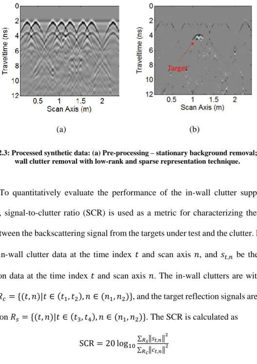
inspection; (b) hyperbolic distortion in GPR B-Scan image [112]. ... 21 Figure 2.1: TWR imaging scenario ... 51 Figure 2.2: Synthetic data: (a) Geometry structure; (2) Raw TWR image. ... 54 Figure 2.3: Processed synthetic data: (a) Pre-processing – stationary background

removal; (b) In-wall clutter removal with low-rank and sparse representation

technique. ... 55 Figure 2.4: Processed simulation data using pattern matching. ... 56 Figure 2.5: Field test data: (a) A hard disk attached on the wall; (b) TWR

scanning from the other side of the wall; (c) MALA concrete imaging system;

(14)

Figure 2.6: Processed field test data: (a) Pre-processing – stationary background

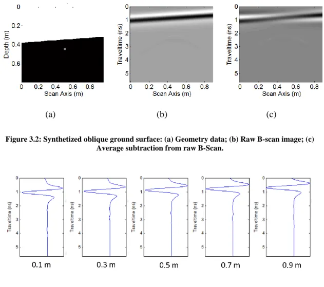
removal; (b) In-wall clutter suppression. ... 58 Figure 2.7: Processed field test data using pattern matching. ... 59 Figure 3.1: Ground clutter removal process ... 71 Figure 3.2: Synthetized oblique ground surface: (a) Geometry data; (b) Raw

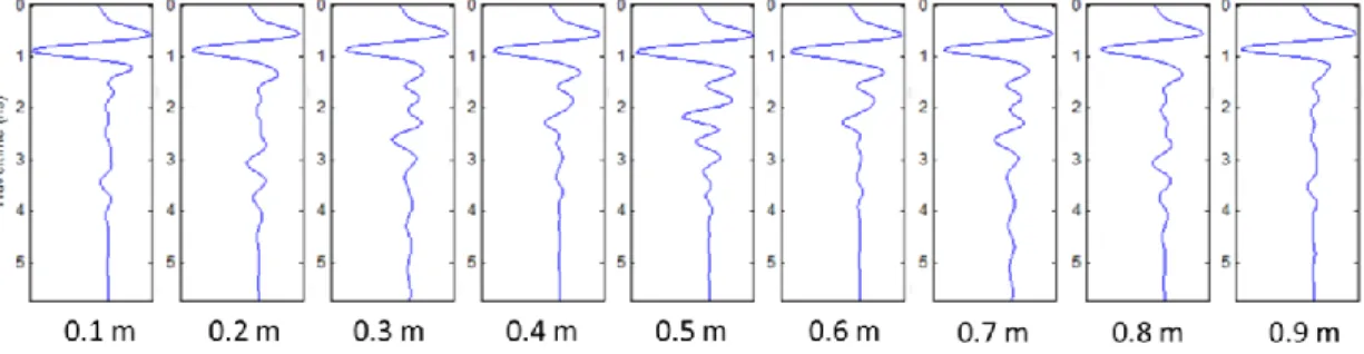
B-scan image; (c) Average subtraction from raw B-Scan. ... 74 Figure 3.3: Synthesized oblique ground surface: A-Scan trace at various

locations along scan axis. ... 74 Figure 3.4: Synthetic oblique ground surface: (a) Aligned B-Scan; (b) Clutter

removal using average subtraction; (c) Clutter removal using proposed method. ... 75 Figure 3.5: Synthetic rough ground surface: (a) Geometry data; (b) Raw B-scan

image; (c) Average subtraction from raw B-Scan. ... 76 Figure 3.6: Synthesized rough ground surface: A-Scan trace at various locations

along scan axis. ... 77 Figure 3.7: Synthetic rough ground surface: (a) Aligned B-Scan; (b) Clutter

removal using average subtraction; (c) Clutter removal using the proposed

method... 77 Figure 3.8: Lab sandbox test: (a) Geometry data; (b) Raw B-scan image; (c)

Average subtraction from raw B-Scan. ... 79 Figure 3.9: Lab sandbox test: (a) Aligned B-Scan; (b) Clutter removal using

average subtraction; (c) Clutter removal using the proposed method. ... 79 Figure 4.1: GPR system diagram: (a) High Speed UWB GPR System; (b) UWB

Pulse Generator; (c) UWB Horn Antenna; (d) Reflection Loss of the UWB

Horn Antenna. ... 89 Figure 4.2: Measurement setup (a) rebar in air; (b) rebar in concrete; (c) Two

horn antennas. ... 90 Figure 4.3: Ballast Test Configuration: (a) Test Platform; (b) Subsurface

Construction. ... 91 Figure 4.4: Raw B-scan images of (a) rebar in air; (b) Two rebars in a concrete

(15)

Figure 4.5: Rebar-in-Air B-scan images after preprocessing: (a) Reference trace subtraction and a LPF filtering; (b) Reference trace subtraction, LPF filtering

and trace averaging operations. ... 92 Figure 4.6: B-Scan images for ballast setup: (a) Raw B-Scan image; (b) B-Scan

image upon preprocessing... 93 Figure 4.7: Pulse peak point shift on different trace index = 1000, 1200, 1400,

1600, 1800, 2000, 2200... 95 Figure 4.8: Entropy data of One Rebar in Air B-Scan. ... 96 Figure 4.9: Entropy analysis along pulse time index (Y-axis) of rebar in-air data:

(a) B-Scan image; (b) Entropy data. ... 101 Figure 4.10: Entropy analysis along trace index (X-axis) of rebar in air B-scan:

(a) B-Scan image; (b) Entropy data. ... 102 Figure 4.11: 2D entropy analysis for B-scan images of a) rebar in air and b)

rebars in concrete. ... 103 Figure 4.12: STFT analysis to correct the singular region detection: (a) STFT

result of one rebar data at x=1.1m; (b) STFT result of two rebar data at x=1.5m. ... 104 Figure 4.13: Final singular region for B-scan images of a) rebar in air and b)

two rebars in concrete. ... 104 Figure 4.14: (a) Rebar in air B-scan image; 2D entropy and STFT analysis

results of traces at (b) left side, (c) middle and (d) right side of rebar area. ... 105 Figure 4.15: (a) Rebars in concrete B-scan image; 2D entropy and STFT

analysis at (b) left rebar and (c) right rebar. ... 107 Figure 4.16: Entropy analysis of ballast data: (a) Entropy along Travel time

index (Y-axis); (b) Entropy along Scan Axis (X-axis). ... 108 Figure 4.17: 2-D entropy analysis for B-Scan image of ballast platform. ... 109 Figure 4.18: STFT analysis result of trace at x = 2.5 m. ... 110 Figure 4.19: Final moisture region detection result based on entropy and STFT

analysis. ... 110 Figure 5.1: GPR system diagram: (a) High Speed UWB GPR System; (b)

Digitizer Configured in SAR Mode; (c) UWB Pulse Generator; (d) UWB

(16)

Figure 5.2: Unsupervised algorithm for detecting region of interest in ballast

layer... 120 Figure 5.3: Amplitude spectrum of GPR A-Scan trace. ... 121 Figure 5.4: Hilbert transform for signal power characterization: (a) GPR A-Scan

trace; (b) GPR A-Scan envelope. ... 123 Figure 5.5: Signal decomposition for identification of backscattering from

different sources: (a) Direct coupling signal; (b) 1st backscattering pulse; (c)

2nd backscattering pulse. ... 125 Figure 5.6: Railroad ballast lab test configuration: (a) Test platform; (b)

Subsurface structure. ... 128 Figure 5.7: B-Scan image from lab tests: (a) Raw B-Scan image; (b)

Pre-processed B-Scan image. ... 129 Figure 5.8: Signal Magnitude Characterization through Hilbert Transform: (a)

B-Scan image plotted using signal magnitude data; (b) Systematic background signals identified through decomposition method; (c) A sample A-Scan trace

waveform. ... 130 Figure 5.9: B-Scan image for ballast layer: (a) Ballast layer; (b) Enhanced

ballast layer. ... 131 Figure 5.10: Entropy analysis of ballast data of Figure 5.8(b): (a) Entropy along

Travel time index (y-axis); (b) Entropy along Scan Axis (x-axis). ... 132 Figure 5.11: 2D entropy analysis of the B-Scan image collected from the test

platform. ... 132 Figure 5.12: GPR System configuration during field tests. ... 134 Figure 5.13: Site pictures: (a) Metro St. Louis MetroLink Blue line; (b) Railroad

ballast. ... 135 Figure 5.14: (a) Field test raw B-Scan image; (b) Pre-processed B-Scan image. ... 136 Figure 5.15: (a) Field test B-Scan image obtained from signal magnitude ; (b)

cross-tie marked by signal decomposition; (c) A-Scan signal at x = 3.8 m... 136 Figure 5.16: B-Scan image for ballast layer: (a) Ballast layer; (b) Enhanced

(17)

Figure 5.17: Entropy analysis of ballast data of Figure 5.15(b) along: (a) Travel

time axis and (b) Scan Distance axis. ... 138

Figure 5.18: Automatic suspicious fouled ballast regions marked by white rectangle. ... 139

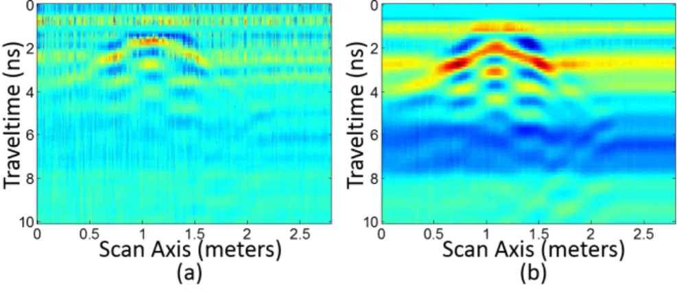
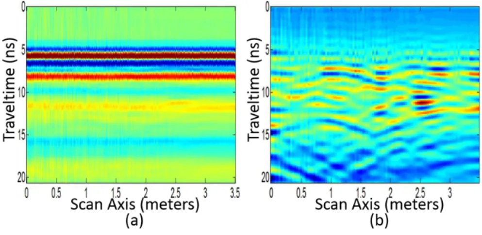
Figure 6.1: One pair of transceiver antennas in multi-static GPR configuration. ... 148

Figure 6.2: WST-SMA Migration Flow Chart. ... 151

Figure 6.3: Principle of BPA for monostatic GPR: (a) Distance between antenna and target in scene space; (b) Wave propagating time from antenna to target; (c) Time domain data points back projected to scene space. ... 152

Figure 6.4: Implementation of BPA for ground-coupled monostatic GPR ... 154

Figure 6.5: Ground-coupled multistatic GPR configuration. ... 161

Figure 6.6: Ground-coupled multistatic GPR imaging. ... 162

Figure 6.7: Air-coupled multistatic GPR configuration. ... 165

Figure 6.8: Air-coupled multistatic GPR imaging. ... 166

Figure 6.9: Ground-coupled multistatic GPR testing setup – three buried targets. ... 172

Figure 6.10: Ground-coupled multistatic GPR raw B-Scan – three buried targets: (1) Tx1-Rx1 pair; (2) Tx1-Rx5 pair. ... 173

Figure 6.11: Ground-coupled multistatic GPR migrated B-Scan – three buried targets: (1) Tx1-Rx1 pair; (2) Tx1-Rx5 pair. ... 174

Figure 6.12: Ground-coupled multistatic GPR migrated B-Scan using proposed multistatic imaging method – three buried targets ... 175

Figure 6.13: Ground-coupled multistatic GPR testing setup – three buried targets. ... 176

Figure 6.14: Ground-coupled multistatic GPR raw B-Scan – congested pipes: (1) Tx1-Rx1 pair; (2) Tx1-Rx5 pair. ... 177

Figure 6.15: Ground-coupled multistatic GPR migrated B-Scan – congested pipes: (1) Tx1-Rx1 pair; (2) Tx1-Rx5 pair. ... 178

Figure 6.16: Ground-coupled multistatic GPR migrated B-Scan using proposed multistatic imaging method – congested pipes. ... 178

(18)

Figure 6.17: Air-coupled multistatic GPR testing setup – three buried targets. ... 179 Figure 6.18: Air-coupled multistatic GPR migrated B-Scan using proposed

multistatic imaging method – three buried targets ... 180 Figure 6.19: Air-coupled multistatic GPR migrated B-Scan upon clutter removal

– three buried targets ... 180 Figure 6.20: Air-coupled multistatic GPR testing setup – congested pipes. ... 181 Figure 6.21: Air-coupled multistatic GPR migrated B-Scan using proposed

multistatic imaging method – congested pipes. ... 181 Figure 6.22: Air-coupled multistatic GPR migrated B-Scan upon clutter removal

(19)

CHAPTER 1:INTRODUCTION

1.1.Non-destructive Testing Problem

According to a 2012 Federal Transit Administration report [1], one-third of the nation’s transit assets are at or have exceeded their expected useful life. More than 40% of bus assets and 25% of rail transit assets are in marginal or poor conditions. The level of capital investment required to attain a state of good repair in the nation’s transit assets is projected to be $77.7 billion. Rail transit assets exceeding their useful life can result in asset failures, which can increase the risk of catastrophic accidents, disrupt service, and strain maintenance departments.

The United States also contains a road network dating to 1940 with more than 570,000 bridges in service. With 3.8 trillion vehicle-kilometers per year, the US roadway infrastructure is considered one of the largest in the world [2]. The average interstate bridge is roughly 40 years old while most bridges are more than 50 years old. In 2013 American Society of Civil Engineering (ASCE) report [3], the accumulated GPA of America’s Infrastructure is rated as D + only, which indicates that “the infrastructure is in poor to fair condition and mostly below standard, with many elements approaching the end of their services life. A large portion of the system exhibits significant deterioration. Condition and capacity are of significant concern with strong risk of failure”. It is also reported that one in nine of the nations’ bridges are rated as structurally deficient. By 2030, that number will double without substantial bridge replacement. The Federal Highway Administration (FHWA) estimates that to eliminate the nation’s bridge deficient backlog by 2028, $20.5 billion annually investment is needed, while only $12.8

(20)

billion is being spent currently. For roads improvements, $170 billion in capital investment would be needed on an annual basis, while the current level is only $91 billion.

Infrastructure can suffer from various defects, such as cracks, spalling, scaling, honeycomb, voids, delamination, insufficient cover, corrosion of rebar, etc. Early and accurate detection, localization and assessment of damages or defects in infrastructure are of great values for scheduling maintenance and rehabilitation activities, and can significantly reduce the damage progression and maintenance costs. To secure the transportation infrastructure safety and cut the maintenance cost, it is critically important to develop effective and efficient testing technologies for the infrastructure structural condition inspections.

Conventional techniques for infrastructure condition assessment, including drilling testing, core sampling, corrosion (half-cell) potentials, acoustic/hammer testing and chloride ion measurements, etc., are destructive, low efficient, low coverage, labor intensive, time consuming, and disturbing to normal traffic. These drawbacks limit their applications for infrastructure inspection during the construction and lifetime maintenance.

Presently, innovative non-destructive testing (NDT) technologies are increasingly adopted by many transportation agencies. Among all non-destructive testing (NDT) techniques, Ground Penetrating Radar (GPR) is deemed as one of the most effective and promising tools enabling subsurface structural characterizations [4]-[5]. As an easily deployed and highly efficient NDT methodology, GPR has been explored in

(21)

various case studies, such as rebar detection [6]-[7], bridge deck inspection [8]-[9], soil moisture assessment [10]-[11], railroad ballast monitoring[12]-[14], underground utility mapping [15]-[16], asphalt pavement inspection [17]-[18], etc. Figure 1.1 shows some testing scenarios of GPR applications for transportation infrastructure inspection.

(a) (b) (c)

(d) (e)

Figure 1.1: GPR explored in various case studies for non-destructive underground infrastructure inspection: (a) asphalt pavement inspection; (b) bridge deck inspection [19]; (c) rebar detection;

(d) underground utilities mapping for smart city; (e) railroad ballast condition assessment.

1.2.Background of Ground Penetrating Radar

1.2.1.History and Applications

GPR is a geophysical method that uses radar pulses to image the subsurface [20]. The most common form of GPR measurements deploys a transmitter and a receiver in a fixed geometry, which are moved over the surface to detect reflections from subsurface features [4].

(22)

The first use of electromagnetic signals to determine the presence of remote terrestrial metal objects is generally attributed to Hiilsmeyer in 1904. The first patent for a system designed to use continuous-wave radar to locate buried objects was submitted by Leimbach, G. and Löwy, H. in 1910 [21]. A patent for a system using pulsed techniques rather than continuous waves was filed in 1926 by Hülsenbeck [22], leading to improved depth resolution. A glacier's depth was measured using GPR in 1929 by Stern, W. [23].

Pulsed radar were further developed from the 1930s as a subsurface sensing methodology for glacier [24], ice [25], salt deposits [26], desert formation [27], tunnel rocks [28] and coal layer [29]. Renewed interests and developments in this field were generally starting from the 1970s, when military applications began driving research and the lunar investigations were in progress. From the 1970s until the present day, the range of applications has been expanding steadily. Commercial applications followed and the first affordable consumer equipment was sold in 1985 [23].

Recent research progress has been continuously driving and expanding the applications of GPR. Now the GPR techniques and methodologies have been used widely in the following applications: archaeological investigations [30], borehole inspection [31], bridge deck analysis [32], building condition assessment [33], detection of buried mines (anti-personnel and anti-tank) [34]-[37], evaluation of reinforced concrete [38], geophysical investigations [39], earthquake and snow avalanche victims detection [40]-[42], underground utilities detection and mapping [43]-[46], planetary exploration [47],

(23)

rail track and bed inspection [48], road condition survey[49], security applications [50]-[51], snow, ice and glacier [52]-[53], timber condition [54], tunnel linings [55], etc.

1.2.2.Operating Mechanism

In GPR’s operation, the GPR transmitter antenna radiates the electromagnetic (EM) wave into the subsurface structure under testing. The EM wave traveling velocity in the structure is determined primarily by the permittivity or dielectric constant of the subsurface material. When the EM wave hits features or objects that have electrical properties differing from the surrounding medium, it will be reflected and received by the receiver antenna. The reflection coefficient at the interface of two media is 𝑅₂₁, which equals the ratio of the electrical fields of the reflection wave and the incident wave. The 𝑅₂₁ value is determined by the following equation [5]:

𝑅21 =√𝜀1−√𝜀2

√𝜀1+√𝜀2 (1.1)

where 𝜀1 is the dielectric constant of the upper media and 𝜀2 is the dielectric constant of

the lower media. The dependence of signal traveling velocity and amplitude on the material electrical properties will result in different reflection waveforms. By analyzing the reflection signals, the subsurface structural features can be effectively characterized.

(24)

Figure 1.2: Model depicting the various scattered signals in impulse ground penetrating radar and the scattered signals shown in time domain [56]

An example is illustrated in Figure 1.2. GPR signal transmitted from a transmitter antenna penetrates into the underground media consisting of two layers, a surface layer and a base layer. The reflection signal back from the media is picked up by a receiver antenna. At each interface between two adjacent layers, some of the signal is reflected, while some of the signal penetrates into the next layer. The reflection signal in this example comprises of following four types of echoes:

 𝐴₀: the signal directly propagates from the transmitter antenna to the receiver antenna, which is called direct coupling signal or end reflection signal.

 𝐴1: the signal reflected from the top surface of the first layer or the surface layer.  𝐴₂: the signal reflected from the interface between the surface layer and the base

layer.

(25)

The amplitude and the time delay of the various reflection pulses 𝐴₁, 𝐴₂ and 𝐴₃ are determined by the dielectric constant and thickness of the media. Therefore, by measuring the amplitude and time delay of different echoes, the dielectric constant of the material, thickness of the layer and depth of the target can be calculated.

During the GPR inspection, the transmitter antenna and receiver antenna move over the underground target. At each scanning position, the receiver antenna collects a 1-D signal. This 1-D signal is called A-Scan trace. As the GPR inspection goes on, a group of A-Scan traces is collected along the scanning direction. Upon assembling all the A-Scan traces, a B-Scan image is produced. Finally, if multiple parallel B-Scan images are collected when moving the antennas over a regular grid, a 3-D data matrix can be recorded, which is called a C-Scan.

1.2.3.System Architecture: Impulse Radar, SFCW Radar and FMCW Radar

From GPR imaging scheme aspect, impulse radar, stepped frequency continuous wave (SFCW) radar and frequency modulation continuous wave (FMCW) radar are three typical architectures for GPR system [56].

Figure 1.3 shows a basic diagram of an impulse radar system. An ultra-wideband (UWB) pulse is generated by UWB pulse generator and transmitted out of the transmitter antenna (TX). The pulse penetrates into the ground and reaches out to the target. Some of this pulse scatters back from the target and travels back to the receiver antenna (RX). The received pulse is amplified by a low noise amplifier (LNA) and sampled by an analog-to-digital converter (ADC) unit, such as oscilloscope or digitizer. The digital GPR pulse is then stored and processed by a host computer. By measuring the time difference

(26)

between the time instances of transmitting the pulse and receiving the pulse, the down range of the target can be calculated.

Figure 1.3: Block diagram of basic impulse GPR system [57].

Figure 1.4: Block diagram of SFCW radar system [58].

Figure 1.4 illustrates the block diagram of SFCW radar system. Continuous wave radar transmits a frequency sweep over a fixed bandwidth. In frequency domain, the

(27)

continuous wave changes by fixed step ∆𝑓. The received signal is acquired as a function of frequency by the data acquisition unit. To achieve an ultra-wide bandwidth, all the frequencies are swept from a set beginning to an end frequency. The amplitude and phase of the received signal at each frequency tone are compared with the transmitted signal to obtain the frequency response of the underground targets. Then the frequency response data is processed by a window function and transformed to time domain signal by inverse Fourier transformation.

Figure 1.5: Simplified block diagram of a coherent linear FMCW radar system [57].

Figure 1.5 depicts the simplified block diagram of a FMCW radar system. The FMCW radar transmits the continuous wave which is frequency modulated with a linear sweep. The sweeping carrier frequency is controlled by a voltage-controlled oscillator (VCO) over a chosen frequency range. At the receiver end, the backscattered wave is mixed with the emitted wave. The difference in frequency between the transmitted and received wave is a function of the depth of the target. By characterizing the frequency difference, the range to the target can be calculated.

(28)

1.2.4.Height of Antenna: Ground-Coupled GPR and Air-Coupled GPR

From the height of antennas aspect, GPR system can be classified as ground-coupled GPR and air-ground-coupled GPR.

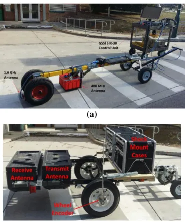
For the ground-coupled GPR system, antennas are installed at close proximity to the ground surface. For this type of GPR, it has higher detecting sensitivity and low signal loss. However, the antennas may hit the ground obstacles and even may not be deployable for hazardous areas like landmine detection scenario. Figure 1.6(a) shows the GSSI SIR-30 GPR system [59] under ground-coupled configuration as an example of ground-coupled GPR.

(a)

(b)

Figure 1.6: GPR antenna configuration: (a) GSSI SIR-30 ground-coupled GPR system; (b) UVM air-coupled impulse GPR system.

(29)

For the air-coupled GPR system, large standoff distance exists between the antennas and ground surface. Such configuration makes the system’s movement has higher flexibility, so the air-coupled GPR is easily deployed and good for high-speed survey. Moreover, since the antennas do not touch the ground, the risk of entering dangerous or hazardous areas for radar operators is reduced. However, due to the large standoff distance above the ground surface, the signal loss is large during the propagation in the air. Figure 1.6(b) provides an example of air-coupled GPR system, an air-coupled high-speed dual-channel impulse ground penetrating radar [60] designed by UVM.

1.2.5.Spatial Offset between Antennas: Monostatic, Bistatic and Multistatic

From the number of antennas and separation distance between antennas aspect, the GPR system can be categorized as monostatic GPR, bistatic GPR and multistatic GPR.

Figure 1.7 illustrates the antenna configuration of those three types of GPR systems. Monostatic GPR is a GPR system in which the transmitter and receiver are collocated [61]. Bistatic radar is the GPR system comprising a transmitter antenna and a receiver antenna that are separated by a distance [62]. The separation distance should be comparable to the expected target distance, otherwise such bistatic GPR can be simplified to a monostatic GPR. Multistatic GPR system contains multiple spatially diverse monostatic radar or bistatic radar components with a shared area of coverage [63]. For example, the multistatic GPR shown in Figure 1.7 has two transmitter antennas and two receiver antennas, so it contains 2 × 2 = 4 components pairs. Each of the components pairs involves a different bistatic angle and target radar cross section. Upon the data

(30)

fusion between each component pair, the spatial diversity afforded by the multistatic GPR system allows for different aspects of a target being viewed simultaneously. Information gained from various antenna pairs and multiple radar cross sections can give rise to a number of advantages over conventional monostatic or bistatic GPR systems [64], such as higher signal-to-noise ratio (SNR), lower shadowing effects, high detection rate, better robustness, etc.

Figure 1.7: Antenna configuration of monostatic GPR, bistatic GPR and multistatic GPR.

1.2.6.Critical Specifications

Range resolution and penetrating depth are two critical specifications for a GPR system.

Range resolution for a GPR system is defined as the minimum detectable or observable distance difference between two targets [57]. For the impulse radar system, targets separated by half of the pulse width time 𝑇_𝑝 can be distinguished. The theoretical range resolution of an impulse GPR system can be calculated by:

𝜌_𝑟 =𝑣𝑒𝑙𝑜𝑐𝑖𝑡𝑦×𝑇𝑝

2 =

𝑐𝑇𝑝

(31)

where 𝑐 is the speed of light in air and 𝜀_𝑟 is the dielectric constant of the subsurface media. Therefore, the narrower the width of the pulse is, the better range resolution an impulse GPR system has.

For a continuous wave (SFCW or FMCW) GPR system, the range resolution is determined by the bandwidth 𝐵𝑊𝑡𝑥 of the transmitting signal instead of the pulse width,

which can be calculated by the following equation: 𝜌_𝑟 =𝑣𝑒𝑙𝑜𝑐𝑖𝑡𝑦

2𝐵𝑊_𝑡𝑥 = 𝑐

2𝐵𝑊_𝑡𝑥√𝜀 (1.3)

Therefore, a GPR system with larger signal bandwidth has a better range resolution. Furthermore, according to Eq. (1.2) and Eq. (1.3), for a specific GPR system, the same transmitting signal has a better resolution when the subsurface media has a larger dielectric constant. Thus, when scanning a subsurface region with larger dielectric constant, to decrease the hardware cost while achieve the certain range resolution, a GPR system with smaller bandwidth can be deployed.

The second critical specification of a GPR system is the penetrating depth, which is determined by central frequency of the GPR system. According to EM wave theory, if the GPR signal’s frequency is high, the penetrating depth is low. On the contrary, if the GPR signal’s frequency is low, the penetrating depth increases. Therefore, the tradeoff between the range resolution and penetrating depth exists when choosing the GPR signal and antennas.

The higher the frequency of the GPR signal and the antenna, the shallower into the ground it will penetrate, while it can see smaller targets, for instance, the rebar in bridge deck. Conversely, a GPR system with low frequency signal and antenna is good

(32)

for deep but big targets, such as underground utility pipes. Thus, choice of antenna and signal frequency is one of the most important factors in GPR survey design. Table 1.1 provides a reference for various transportation infrastructure applications and corresponding appropriate choices of GPR signal and antenna.

Table 1.1: Antenna frequency, approximate depth penetration and appropriate application [66].

Appropriate Application Primary Antenna Choice Secondary Antenna Choice Depth Range (Approximate) Structural Concrete, Roadways,

Bridge Decks 2600 MHz 1600 MHz 0-0.3 m (0-1.0 ft) Structural Concrete, Roadways,

Bridge Decks 1600 MHz 1000 MHz 0-0.45 m (0-1.5 ft) Structural Concrete, Roadways,

Bridge Decks 1000 MHz 900 MHz 0-0.6 m (0-2.0 ft) Concrete, Shallow Soils,

Archaeology 900 MHz 400 MHz 0-1 m (0-3 ft)

Shallow Geology, Utilities,

UST's, Archaeology 400 MHz 270 MHz 0-4 m (0-12 ft) Geology, Environmental, Utility, Archaeology 270 MHz 200 MHz 0-5.5 m (0-18 ft) Geology, Environmental, Utility, Archaeology 200 MHz 100 MHz 0-9 m (0-30 ft) Geologic Profiling 100 MHz MLF (16-80 MHz) 0-30 m (0-90 ft) Geologic Profiling MLF (16-80 MHz) None Greater than 30 m (90 ft)

(33)

1.3.GPR Signal Processing Problems and Methodologies

In this section, general and conventional GPR signal processing problems and methodologies are introduced. Methodologies that are more sophisticated will be described and discussed in further chapters when specific GPR signal processing problems are addressed and investigated.

Cassidy, N. J. in 2009 [67] summarized the typical GPR data processing flow by 11 steps. Considering the GPR research has kept progressing since 2010s and the focus of this dissertation is GPR signal processing instead of general data processing, we emphasized a few of the steps in Cassidy’s flow, added some new steps into it and reorganized the sequence with each of the steps in their most relevant order as: (1) Editing and Rubber-banding; (2) Dewow; (3) Time-zero correction; (4) Range Filtering and Cross-Range Filtering; (5) Deconvolution; (6) Migration; (7) Attribute analysis; (8) Gain Adjustment; (9) Image analysis; (10) Region of Interest Detection. Each of these signal processing steps will be elaborated in this chapter.

1.3.1.Trace Editing and Rubber-banding

In GPR survey, caused by overenthusiastic triggering, external noise sources, equipment failure or malfunction, occasional traces may be corrupted or missed. Existence of bad traces will impair the processing results of further GPR signal processing steps. The “editing” is to correct the bad or poor data and reorganize the A-Scan traces in the data file. Interpolation between good traces is often performed to compensate the missed traces or replace the corrupted traces [68]-[69].

(34)

Similarly to trace editing, rubber-banding is also a process to modify the A-Scan traces, which corrects the GPR data to ensure spatially uniform increments in GPR scanning direction. For distance triggered GPR system, equidistant data collection is required for subsequent signal processing steps, such as migration. To ensure the good data registration, a series of marker points at know distances are recorded during the GPR survey. If the traces corruption or missing happens, the corrupted section is interpolated between to known marker points and then resampled to produce a good section with equally spaced traces [70]-[72].

1.3.2.Dewow

‘Wow’ is caused by the swamping or saturation of the recorded signal by the strong direct coupling wave or air-ground surface reflection signal. If the DC signal bias exists in the A-Scan trace, the low-frequency component will distort the spectrum of the A-Scan in frequency domain, which affects the subsequent spectral processing steps in frequency domain [73]. Dewowing step reduces the DC bias or the low-frequency components from the GPR signal and adjusts the mean of the A-Scan trace to zero. This process can be implemented in two ways. In the first way, the DC bias or component is calculated as the average of the data points on the A-Scan trace and then subtracted from the A-Scan trace. Alternatively, a high-pass filter with a cut-off frequency that is below the bandwidth of the recorded signal is performed to filter out the low frequency or DC component in the A-Scan trace [74]-[75].

(35)

1.3.3.Time-zero correction

If the antenna platform is fixed, the arrival time instance of direct coupling signal in each A-Scan trace should be identical. However, thermal drift, electronic instability, cable length differences and variations in antenna air-gap can cause shifting in the time instance of direct coupling signal [76]. The misalignment of the time-zero correction has an effect on the position of the ground surface reflection and the target reflection, thus, it is necessary to adjust the A-Scan traces to a common time-zero position before subsequent processing steps are performed. Typically, the direct coupling signal in one A-Scan trace is chosen as the reference. The time shifting between the direct coupling waves in different A-Scan traces are calculated by cross-correlation [77]-[78]. Then the time shifting is compensated to each A-Scan trace so that all the A-Scan traces are matching with a common time-zero position.

1.3.4.Range Filtering and Cross-Range Filtering

Generally, GPR filtering can be classified into two types: range filtering along individual A-Scan trace and cross range filtering across a number of A-scan traces.

The goal of the range filtering is removing the noises in A-Scan traces to improve the SNR of GPR signal. Moving average filter [79] is one of the typical temporal filters. The moving average is calculated as the weighted mean of data points within a specified window. The moving average filter is good for removing excessive higher-frequency noise from the data such as radio frequency interference from communication devices [67]. Median filter [80]-[82] is a nonlinear digital filtering technique, often used to remove spikes and salt and pepper noise from GPR A-Scan trace. The median filter runs

(36)

through the signal point by point, replacing each data point with the median of its neighboring data points across a specified window. While moving average filter and median filter are both attempted in time domain, low-pass filter (LPF), high-pass filter (HPF) and band-pass filter (BPF) are the other type of range filter along A-Scan traces performing in frequency domain [83]-[86]. The LPF can remove the high-frequency noise, and the HPF can suppress the DC bias and low frequency noise. The BPF can be considered a cascade combination of the LPF and HPF performing on the GPR A-Scan signal. The cutoff frequency of each filter can be determined based on bandwidth of the transmitting signal. Joint time-frequency (JTF) analysis [87]-[88] is also applied to suppress the noise components in GPR A-Scan trace. As one of the JTF analysis methods, wavelet transform [89] decomposes the GPR A-Scan into the combination of various signal atoms, eliminates the noise components and reconstructs the GPR signal with the residual signal components.

Radar clutter is the undesired receiving signal other than the scattering signal from the target. Cross-range filtering is aiming to improve the signal-to-clutter ratio (SCR) of GPR signal by suppressing the radar clutter in GPR image. Time gating [90]-[92] is one of the earliest clutter removal methods. In the time gating method, a windowing function is defined to null the signal segments over the time intervals where different signal traces exhibit a high similarity, which facilitates clutter signal removal. Average (or background) subtraction [93]-[94] is a widely used method to remove the ground reflection. Assuming the clutter in each A-Scan shows high similarity, the average subtraction method calculates the average of the first several A-Scan waveforms

(37)

as the background and then subtracts this average value from the B-Scan image. Spatial filtering method [95]-[96] utilizes the same assumption to filter out the clutter data corresponding to the ground surface reflection. Considering the reflection signal from the buried object with limited spatial extent varies in different A-scan traces, a spatial filter is thus applied along the antenna moving direction to mitigate the spatial zero-frequency and low-zero-frequency components corresponding to clutter. Principal component analysis (PCA) [97]-[99] and independent component analysis (ICA) [100]-[101] are also conventional clutter removal methods. PCA and ICA uses the mathematical modeling principle to decompose the signal into different components, and then finds out the components corresponding to object and clutter respectively. The subspace projection approach [102] is based on the reflection energy difference between the ground surface and the buried object. Singular value decomposition (SVD) is performed on the data matrix to identify and remove the ground surface electromagnetic signature.

Differing from the aforementioned GPR signal processing steps (editing, rubber-banding, dewow, time-zero correction and range filtering) which already have well-developed conventional methodologies, the cross-range filtering or clutter removal filtering is still an open research problem. On the other hand, since the SCR of the GPR data is the key to target detection, while GPR signal is heavily contaminated by clutter, clutter removal is also one of the primary objectives in GPR signal processing [21]. Therefore, exploring of clutter removal methodologies that can efficiently and effectively eliminate or suppress the clutter signal component under complex GPR testing scene is still a challenge research topic.

(38)

1.3.5.Deconvolution

Deconvolution is a temporal process that removes the effect of the source wavelet from the recorded A-Scan trace and compresses the recorded GPR wavelet into a narrow and distinct form [103]-[105], which is similar to the idea of pulse compression in general radar signal processing [106]. The deconvolution can effectively improve the resolution of the reflection signal if two primary assumptions can be met extremely. The first assumption is the subsurface is horizontally layered and homogeneous. The second one is the propagating signal should be plane-wave. For GPR testing scene, these are very restricting assumptions as the subsurface is complex and usually inhomogeneous. Moreover, the GPR is a short-range system [57] when scanning some shallowly buried targets, so the GPR signal propagates in near field and can not be modeled as plane-wave. Therefore, the effectiveness of deconvolution technique is not assured if no special handling is performed [107]-[108]. Regularized deconvolution with calibration testing on directly coupling signal [109], metal plate reflection signal in free space [110], and attenuation model [111] is more practical for GPR inspection scene.

1.3.6.Migration

Since the GPR antenna receives the field scattering while moving above the buried object along the inspection direction, the EM waves reflecting back from the same object have different travel times to the GPR antennas at different positions. For instance, as demonstrated in Figure 1.8, for a ground-coupled monostatic GPR system, when the antenna is at location 1, the distance between the target and the antenna is 𝑅₁. Correspondingly, the two-way travel time for the EM wave is 𝑡₁ = 2𝑅₁⁄𝑣, where 𝑣 =

(39)

𝑐/√𝜀𝑟 is the propagation velocity of the EM wave in subsurface media. While antenna

moves to the position right above the target, its range to the target is 𝑅2 and the two-way

signal travel time is 𝑡₂ = 2𝑅₂⁄𝑣. In GPR B-scan image, the object pattern shows a hyperbolic distortion, which impairs the shape of buried target and decreases the cross-range resolution of the GPR B-Scan image. Therefore, one of the most important GPR signal processing steps is to migrate the distorted GPR image to a focused one and reconstruct the true shapes and locations of buried targets.

Figure 1.8: Hyperbolic distortion in GPR image: (a) geometrical layout of GPR inspection; (b) hyperbolic distortion in GPR B-Scan image [112].

(40)

The concept of migration was originally proposed for processing seismic images [113]-[114], and introduced to the GPR imaging thanks to the likenesses between the acoustic and EM wave equations [112]. Conventional migration methods for GPR imaging include the hyperbolic summation, Kirchhoff’s migration, phase-shift migration, frequency-wavenumber (𝜔-𝑘) migration, and back-projection migration.

Hyperbolic summation (HS) migration [115] is a GPR version of the diffraction summation method [116] that has been successfully applied in seismic data processing. The HS migration method assumes the B-Scan image can be modeled as the contribution of finite number of hyperbolas that correspond to different points on the targets. It is implemented as a summation of the diffraction energies along a hyperbolic trajectory operating on spatial domain [117].

Kirchhoff’s migration [118] is also known as reverse-time wave equation migration whose aim is to find the Kirchhoff solution of the wave equation within the propagating medium based on Huygen’s principle [119]-[120]. The Kirchhoff’s migration can produce a good reconstructed radar image for monostatic GPR setup. However, the Kirchhoff’s migration is derived from the zero-offset exploding reflector model [121], so it does not account for the spatial offset between the transmitter antenna and receiver antenna, which make it infeasible for bistatic GPR or multistatic GPR.

Phase-shift migration [122] method iteratively compensates a phase-shift to migrate the wave field to the exploding time of 𝑡 = 0 such that all the scattered waves are mapped back to target scene. The main objective of the phase-shift migration method is to calculate the wave field at 𝑡 = 0 by extrapolating the EM wave in range direction

(41)

with a phase factor [112]. The concept and assumption of the phase-shift migration is similar to Kirchhoff’s migration [123], therefore, it is only designed to work for monostatic GPR configuration.

Frequency-wavenumber (𝜔-𝑘) migration technique is based on the phase-shift migration algorithm, which was first proposed for seismic imaging applications [124] and then adapted to the synthetic aperture radar (SAR) imaging [125]-[130]. This algorithm is also called as seismic migration algorithm, 𝑓-𝑘 migration algorithm, or Stolt migration algorithm (SMA) by different researchers. For simplicity, we call it SMA in this dissertation. The main idea of the SMA is the interpolation operation in the wavenumber-wavenumber domain to obtain the reconstructed image in the scene space. The SMA works faster than the aforementioned migration techniques. Unfortunately, the traditional SMA also fails to consider the spatial offset between the transmitter antenna and receiver antenna, so it can only work for monostatic GPR imaging. Some modified or improved SMAs were proposed in [131]-[132] for multiple-input multiple output (MIMO) radar system claiming the separation between the transmitter antenna and receiver antenna was considered, nevertheless, those modified SMAs are formulated from the models of transmitted signals in air or free space medium. Thus, they do not perform well in subsurface lossy medium [133] for GPR applications.

Back-projection algorithm (BPA) was first introduced as a seismic migration method [113] and then further developed for SAR imaging applications [134]-[137]. The BPA algorithm characterizes the differences in the two-way EM wave propagating distance at different antenna locations and projects the collected data points from the

(42)

recorded time instances back to their true spatial locations in scene space. The primary advantage of BPA is its flexibility in handling the configuration of radar systems. Theoretically, once the exact location of the antenna is measured and the propagating path of the EM wave is determined, BPA can reconstructed the target from the radar image. Therefore, BPA has the potential to be extended to air-coupled bistatic and multistaic GPR system. Secondly, since each of the A-Scan traces is serially processed and back-projected to the entire GPR image independently, the BPA does not require a straight and uniformly sampled synthetic scan aperture [112]. This “independently processing” property of BPA also implies its capability of the real-time imaging as the GPR scanning is undergoing. Thirdly, the BPA can project the GPR time-domain data points back to a specific sub-region of the scene space. For GPR applications where the approximate location of the buried target or the region of interest (RoI) is a priori-knowledge, the BPA can directly imaging the RoI instead of the whole subsurface region. Therefore, using some RoI detection algorithms as the pre-processing, the GPR imaging efficiency of BPA can be improved dramatically.

1.3.7.Attribute Analysis

Attribute analysis extracts the information about the relative reflectivity, amplitude, frequency, phase relationships and statistical features to aid GPR data interpretation.

The basic attribute analysis is performed on the whole A-Scan signal, e.g. mean amplitude, peak amplitude and time delay between two peaks, which can be used for many GPR applications, such as, estimating the dielectric constant of the subsurface

(43)

media [5], [138], the density of the asphalt pavement [139]-[141], the thickness of the asphalt pavement [142]-[143]. Some attribute analysis methods operate on the data points within a time window, e.g. instantaneous amplitude, instantaneous phase and instantaneous frequency. Those instantaneous features have been utilized for estimation of water content [144], detection of subsurface contaminant [145]-[146], detection of fouling railroad ballast [147], etc. Recently, joint time-frequency techniques considering both the temporal features and frequency features have been explored for analyzing and interpreting GPR data, which include empirical mode decomposition (EMD) [148]-[151], short-time Fourier Transform (STFT) [152]-[154], wavelet transform [155]-[157] and curvelet transform [158]-[159], etc.

1.3.8.Gain Adjustment

Gain adjustment modifies the signal amplitude to improve the visualization of the GPR image. Since the data values are manipulated, the relative amplitudes information or phase relationships within the GPR image are changed. Therefore, we would like to perform the gain adjustment as the last GPR signal processing step.

To eliminate the signal attenuation during transmitting in subsurface media and enhance the target scattering signal, a scaling function 𝐴(𝑑) is multiplied to the amplitudes of received signal at different depths. Typically, a deeper 𝑑 corresponds to a larger value of 𝐴(𝑑). Theoretically, for the visual purpose, the scaling function 𝐴(𝑑) can be arbitrary function defining by the GPR operator or user. However, we have to admit that gain adjustment manipulates the data values, so the bias from GPR operator is

(44)

inevitable. Moreover, since the gain is applied to all the data points in the GPR image, both the target signal and noises are amplified simultaneously in an indiscriminate way. Here, a practical gain function based on characterizing the signal propagating loss in the subsurface media [10], [13] is described as an example. For the signal penetration in a uniform or homogeneous media, the attenuation is linearly proportional to the penetrating depth. The gain function of signal transmitted in the media can be characterized as

𝑔(𝑚) = 𝑔(1) +𝑔(𝑀)−𝑔(1)

𝑀−1 (𝑚 − 1), 𝑚 = 1,2, … , 𝑀 (1.4)

where 𝑚 represents the index of the sample along the range direction (penetrating depth) in B-Scan image while 𝑔(𝑚) (unit: dB) indicates signal attenuation. Assuming the incident signal voltage amplitude at the ground surface is 𝑉(0) and the voltage amplitude at depth 𝑑 is 𝑉(𝑑), we have

20 log (𝑉(0)

𝑉(𝑑)) = 𝛼 · 𝑑 (1.5)

where 𝛼 is the attenuation coefficient (unit dB/meter) and 𝑑 is the penetrating depth. 𝑉(𝑑) can be derived as

𝑉(𝑑) = 𝑉(0) × 10−𝛼·𝑑20 _(1.6)

The value of 𝛼 can be determined by [160]:

𝛼 = 𝜔√𝜀𝜇 {1₂[√1 + (𝜎 𝜔𝜀) 2 − 1]} 1 2⁄ (1.7)

where 𝜎 is the electrical conductivity of the media, 𝜇 is the permeability of the media, 𝜇 = 𝜇₀ = 4𝜋 × 10−7_{henry/m, 𝜔 = 2𝜋𝑓, 𝜀 is the dielectric permittivity.}

(45)

When the penetrating depth increases by 𝑑 meters, the signal round trip transmission distance increases by 2𝑑 meters. If the signal attenuation/transmitting distance ratio is 𝛼 dB/meter, the round trip signal attenuation is thus 2𝛼 dB. An exponential parameter 𝐴(𝑑) can be multiplied to 𝑉(𝑑) to compensate signal transmission attenuation and make it outstanding from the background. The scaling function 𝐴(𝑑) can be derived based on Eq. (1.6):

𝐴(𝑑) = 102𝛼𝑑20 = 10 𝛼𝑑

10 _(1.8)

1.3.9.Image analysis

Recently, computer vision techniques have drawn the attention of GPR research community for analyzing, interpreting and understanding the GPR image. Machine learning techniques were adopted for buried target detection [161]-[163] and signal classification [164]-[165]. Pattern recognition techniques [166]-[167] were utilized to detect the hyperbolas representing the buried targets in the GPR image. The popular and sparking deep learning methodologies were also explored by GPR researchers for buried target detection [168]-[172] and classification in GPR image [173]-[175]. The accuracy of the detection and classification by machine learning or deep learning techniques is primarily dependent on the amount of the training data. However, differing from computer vision applications, the images or datasets for radar applications are not often open to the academia community. Therefore, the limitation of the data source as training dataset could be an obstacle to the transition of deep learning application from computer vision to radar imaging.

(46)

1.3.10.Region of Interest Detection

For the aforementioned GPR signal processing steps, the algorithm computational cost is always an issue, especially for GPR field test data whose data size could be extremely large. In a large radargram, the targets or the scatters of interests are typically distributed sparsely in the imaging region. Therefore, reducing the data scope to sporadically distributed singular regions or region of interest (RoI) can facilitate sophisticated post-processing. The RoI detection can be integrated into any GPR signal processing steps as a pre-processing. Then the specific algorithm is only performed on the sub-regions of the GPR image, which can leverage the computation efficiency and minimize the space cost of the algorithm. For instance, for back-projection imaging algorithm, if the RoI is a prior knowledge, the BPA can just be performed on the RoI as the scene space instead of the whole GPR scanning region.

1.3.11.Summary

In this section, the typical GPR signal problems are introduced and the corresponding methodologies are reviewed. Among those problems, trace editing, rubber-banding, time-zero correction and gain adjustment already have standard processing methodologies and protocols. They have already been standardized and integrated into some commercial GPR signal processing software products, such as RADAN by GSSI [179], ObjectMapper by MALA [180], etc. For dewow, deconvolution and attribute analysis, even though no so-called standard algorithm or methodology exists, the state-of-the-art research results can already handle these problems well. Most of well functional methodologies have already been implemented and included in a free

(47)

GPR data processing tool, the MATGPR [181]. However, the clutter removal filtering, region of interest detection and image migration are still open questions lacking of very effective and efficient methodologies. Therefore, they are the major GPR signal processing problems that will be addressed in the following chapters of this dissertation. Please note, image analysis is actually a problem more relevant to computer vision and machine learning research areas, so it is not included in the topics of this dissertation even though it is essential and challenging.

1.4.Objective and Scope

The objective and focus of this dissertation is to investigate the key techniques to tackle with GPR signal processing from three perspectives: (1) Removing or suppressing the radar clutter signal; (2) Detecting the region of interest (RoI) in the GPR image; (3) Imaging the underground target to eliminate or alleviate the hyperbolic distortion and reconstructing the shape of the target with good fidelity.

The first part of this dissertation, consisting of Chapter 2 and Chapter 3, tackles with the clutter removal problems in through-the-wall radar (TWR) imaging and GPR imaging respectively. In Chapter 2, for TWR imaging, in-wall clutter data from rebars or pipes inside the wall is modeled as a low-rank matrix, while the data from the foreground target under testing is modeled as a sparse matrix that lies on top of the in-wall clutter. The in-wall clutter suppression problem for TWR image processing is then transformed into a low-rank and sparse representation optimization problem. A low-rank and sparse representation method is explored and developed to mitigate the in-wall structure reflection so as to leverage behind-wall object detection effectiveness in TWR image

(48)

processing. In Chapter 3, this low-rank and sparse representation based approach is improved and extended to remove the clutter produced by rough ground surface reflection for GPR imaging applications. For rough or non-flat ground surface, the surface clutter components in different A-Scan traces are not aligned on the depth axis. To compensate for the misalignments and facilitate clutter removal, the A-Scan traces in a GPR data matrix are aligned using cross-correlation method. The low-rank and sparse representation technique is then developed to decompose the aligned GPR data matrix into two sub-matrices: a low-rank matrix whose column data records the ground clutter in A-Scan traces, and a sparse matrix that features the subsurface object.

The second part, consisting of Chapter 4 and Chapter 5, explores the methodology for detecting the region of interest (RoI) in the GPR image. Chapter 4 proposes the utilization of two-dimensional (2-D) entropy analysis to narrow down the data scope to the interested regions, which can considerably reduce the computational cost for sophisticated post data processing steps. Joint time-frequency analysis using Short Time Fourier Transform (STFT) is then performed for singular region location detection and refinement. Chapter 5 improves the entropy-based algorithm to automate and facilitate the detection of suspicious fouling ballast regions or Regions of Interest (ROI) within big GPR survey data sets. An analytic method using Hilbert Transform is developed to extract the pulse signal envelope and characterize the scattering signal power. Furthermore, an automatic layer identification method based on signal decomposition is implemented to detect and isolate the ballast region from the ground surface. Finally, the 2-D entropy analysis is performed on the scattering data corresponding to ballast region.

(49)

Such data processing approaches leverage the performance of 2-D entropy analysis and eliminate the need of STFT for singular region identification. The improved methodology can effectively facilitate the post processing and interpretation for large volume of GPR ballast inspection data.

In the third part, Chapter 6, a back-projection imaging algorithm is designed for both ground-coupled multistatic GPR and air-coupled multistatic GPR configurations. Since the refraction phenomenon at the air-ground interface is considered and the spatial offsets between the transceiver antennas are compensated in this algorithm, the data points collected by receiver antennas in time domain can be accurately mapped back to the spatial domain and the targets can be imaged in the scene space with good fidelity. Comparing to the monostatic GPR imaging and bistatic GPR imaging, the multistatic GPR imaging can produce higher signal-to-noise ratio (SNR), lower shadowing effects, high detection rate and better robustness for GPR infrastructure inspection applications. Chapter 7 concludes that the proposed three-stage cascade signal processing methodologies can improve the performance of GPR system. The further work based on this dissertation is also remarked in Chapter 7.

1.5.References

[1] Federal Transit Administration Asset Management Guide, October 2012, FTA

Report No. 0027:

https://www.transit.dot.gov/sites/fta.dot.gov/files/docs/FTA_Report_No._0027.p df

[2] Bettigole, N. and Robinson, R., “Bridge Decks,” American Society of Civil Engineers, New York, (1997).

[3] 2013 Report Card for America’s Infrastructure, American Society of Civil Engineers: http://2013.infrastructurereportcard.org/