Volume 34
Number 517
Beef-cattle production functions in forage
utilization
Article 1
July 1963
Beef-cattle production functions in forage
utilization
Earl O. Heady
Iowa State University of Science & Technology
Glenn P. Roehrkasse
Iowa State University of Science & Technology
Walter Woods
Iowa State University of Science & Technology
J. M. Scholl
Iowa State University of Science & Technology
Follow this and additional works at:
http://lib.dr.iastate.edu/researchbulletin
Part of the
Agriculture Commons
,
Agronomy and Crop Sciences Commons
,
Animal Sciences
Commons
,
Economics Commons
, and the
Sociology Commons
This Article is brought to you for free and open access by the Iowa Agricultural and Home Economics Experiment Station Publications at Iowa State University Digital Repository. It has been accepted for inclusion in Research Bulletin (Iowa Agriculture and Home Economics Experiment Station) by an authorized editor of Iowa State University Digital Repository. For more information, please contactdigirep@iastate.edu.
Recommended Citation
Heady, Earl O.; Roehrkasse, Glenn P.; Woods, Walter; and Scholl, J. M. (1963) "Beef-cattle production functions in forage utilization," Research Bulletin (Iowa Agriculture and Home Economics Experiment Station): Vol. 34 : No. 517 , Article 1.
Beef-Cattle Production Functions
in Forage Utilization
by Earl O. Heady, Glenn P. Roehrkasse, Walter Woods and J. M. Scholl
Department of Agronomy Department of Animal Science
Department of Economics and Sociology
AGRICULTURAL AND HOME ECONOMICS EXPERIMENT STATION
IOWA STATE UNIVERSITY of Science and Technology
CONTENTS
Summary 883
Introduction ... 885
Scope and objectives of the study ... 885
Empirical results ... 886
Experimental design ... 886
Estimation of the production function . . . .. 887
Gain isoquants ... 889
Ration lines ... . .. 893
Least-cost rations ... 896
Estimation of the time function . . . .. 898
Grade functions ... 903 Profit maximization ... 908 Appendix A Appendix B 917 918
SUMMARY
Little information has existed on substitution rates between pasture forages and corn in a beef-fattening enterprise. Without this knowledge it is difficult to determine which combinations of pasture forage and com would maximize profits. Profits in feeding depend not only on the cost of feed but also on the time of marketing. The pasture forage-corn ration that mini-mizes costs may not necessarily be the ration that maximizes profits, since profits are affected by the time of marketing. Both the quality and the price of beef are subject to change during the beef-fattening period. Consequently, the beef-cattle feeder is confronted with the problem of selecting (a) the least-cost pas-ture forage-corn ration (b) that will place the beef cattle on the market finished to a grade (c) at the time when the expected market price will maximize profits.
A beef-feeding experiment was designed to deter-mine the feed relationships between soilage (fresh-chopped pasture forage) and com. It was conducted at two locations over a period of 3 years -1957, 1958 and 1959. Six different soilage-com rations, ranging from all soilage to 2 parts soilage and 1 part corn, were fed to different lots of feeder steers at each loca-tion. The rations at each location were also fortified with a feed supplement. Stilbestrol was included in the rations at one of the locations. The results of this feeding experiment are based on the performance of 336 head of good-to-choice feeder steers.
Several alternative regression equations, including quadratic, modified Cobb-Douglas and exponential functions, were used in this study to estimate produc-tion surfaces. In each of the funcproduc-tions, an attempt was made to remove the effects of autocorrelation by estimating an autocorrelation coefficient and then mak-ing an autoregressive transformation.
The quadratic functions gave better results than either the modified Cobb-Douglas or the exponential functions. However, more research is needed to deter-mine which functions are best under different situa-tions. In some cases the modified Cobb-Douglas func-tion gave good results. In other cases, it gave increas-ing returns to scale, denotincreas-ing that a small pro-portional increase in the quantity of feed fed results in a more than proportionate increase in beef gain. These results are inconsistent with theory. The ex-ponential functions, which merit further research, gave sigmoid isoquant contours, denoting, first, increasing marginal rates of substitution between feeds and, then, decreasing marginal rates of substitution. Again, these results are inconsistent with logic.
The quadratic production functions for rations with and without stilbestrol and the aggregate function with the stilbestrol and nonstilbestrol rations combined are:
1. With stilbestrol
G=0.11637150C+0.02316051F -0.0000049955C2-0.0000007455F2 +0.000000037 4CF -1.2236046H
II. Without stilbestrol
G=0.14971812C+0.02128774F -0.OOO0122612C2-0.0000007455F2 0.0000037907CF -2.2005042H III. The aggregate function
G=0.13628727 +0.02193828F -0.00OO0819C2-0.00000063F2 -0.00000253CF -1.75011550H
In these equations, G refers to pounds of beef gain, C refers to pounds of corn, F refers to pounds of soilage, and H refers to the deviations of the average maximum temperature of each observation interval from the mean maximum temperature for the over-all feeding period. From these production functions, the basic input-output relationships can be derived.
The marginal rates of substitution of com for soil-age have been derived for various soilsoil-age-corn rations at various levels of beef gain. The marginal rates of substitution indicate, for a given level of gain, the pounds of soilage that could be replaced if an addi-tional pound of com were added to the ration. For 100 pounds of beef gain, the marginal rate of sub-stitution of com for soilage is 6.57 for the 20:1 soilage-com ration with stilbestrol; it is 5.17 for the 2:1 ration. For the same level of gain, the marginal rate of sub-stitution of com for soilage is 8.11 for the 20:1 soilage-com ration without stilbestrol and is 7.36 for the 2:1 ration. The marginal rates of substitution of com for soilage are diminishing. Similar results were obtained for higher levels of beef gains.
Time equations, which were derived from estimated soilage-consumption functions, express the total time (T) required to consume a given quantity of com and soilage as a function of the soilage (F) and com ( C) fed. The time equations for the rations with and without stilbestrol are:
I. With stilbestrol
T
=
-558.36128626+0.05781948C+6.7475645 (6,847.57044400 -0.OOOO0523C2-0.82767919C
-0.26107315H+0.29640324F) \o!o
II. Without stilbestrol
T = -1,176.48647060+0.oo763899C
+ 11.436640 (10,582.2245560 -0.OOO01571C2+0.45460922C -3.07787452H+0.17108144F)M.
These equations were used to predict the time re-quired to produce various levels of gain for different soilage-corn rations. The time required to produce a given level of gain, for the rations both with and without stilbestrol, decreases as the proportion of corn in the ration increases. Also, for a given feeding period the maximum level of gain is attained with the heaviest com ration (i.e., the 2:1 soilage-com ration).
The beef steers were graded at definite intervals during the feeding period. After the grade
observa-tions (which were in subjective grade terms) had been coded, a functional relationship that expressed grade as a function of the com and soilage fed was estimated for both the stilbestrol and nonstilbestrol rations. The over-all equations for estimating the grade of beef steers fed various soilage-com rations either with or without stilbestrol are:
I. With stilbestrol
Q=21.67 +O.0024655079C
+O.0000220680F -O.OOO0003510C2 II. Without stilbestrol
Q=21.67 +O.00l6294178C
+O.OOO0270836F -O.OO00000330C2
where Q is the predicted slaughter grade which can be interpreted in subjective grade terms. From these grade functions, the isograde equations, as well as the marginal rates of substitution equations, can be de-rived.
To estimate the profits from feeding different soil-age-corn rations for feeding periods of different lengths with different feed-price assumptions, it was necessary to derive a price function that would esti-mate the price of the beef steers during the feeding period. These price functions represented the grade of the beef steers during the feeding period, as well as the general market price associated with the grade. The estimated price functions were used in the over-all stilbestrol and nonstilbestrol profit functions. The profit equations are:
884 I. With stilbestrol '11'= ( 850.00+0.11637150C+0.02316051F -0.OOOOO49955C2-0.0000007455F2 +0.000000037 4CF -1.2236046H) (0.2500-0.00oo040158F +0.OOO0382807T +O.OO00017537T2-0.oo0oooo048FT) -PcC-PFF -O.2TPs-K
II. Without stilbestrol
'11'= (850.00+0.14971812C+O.0212877 4F -0.OOO0122612C2-0.00oo005775F2 -O.OOO0037907CF -2.2oo5042H) ( O.2500-0.0000004996F -O.0002393978T +0.OOOOO36576T2-0.0000000281FT) -PcC-P};'F -O.2TPs-K
where '11' refers to the profit, Po refers to the price of corn, P),. refers to the price of soilage, Pa refers to the price of the supplement, K is the value of the feeder steer at the beginning of the feeding period, and all of the other symbols are the same as explained for the earlier equations.
Estimated profits from feeding beef steers various soilage-com rations for feeding periods of various lengths under various feed-price assumptions have been tabulated in the text. Usually, for this experiment, the greatest profits are obtained by feeding the heavi-est com ration. However, when the price of soilage is low relative to the price of corn, the most profitable ration includes less corn and more soilage.
The equations and the procedure also are given in the text for obtaining the optimum feeding period for any given soilage-com ration under different feed-price conditions. Similarly, the equations and the pro-cedure are given for obtaining the optimum soilage-com ration with different feed-price assumptions.
Beef-Cattle Production Functions
in Forage Utilization!
by Earl O. HeadYt Glenn P. Roehrkasset Walter Woods and J. M. Scholl
The optimum proportion of land which should be devoted to forage or grasses and grain has long been studied by agriculturists. Similarly, the optimum pro-portion of forage, grain and other feed materials to be included in a livestock ration has been a continuous concern. These are not unrelated problems since, as has been shown elsewhere, the optimum proportion of forage and grain is not independent of the optimum proportion of the two crops grown in the crop rota-tion (and vice versa). 2 For a physical maximum of livestock production from a given land area, the mar-ginal rate of substitution of feeds produced in the crop rotation must equal the marginal rate of substitution of the same feeds used in the livestock ration. Even where attempts are not made to maximize the livestock pro-duct from a given land area, these two sets of marginal rates of substitution are basic to decisions on profit maximizing in growing crops or feeding livestock. 3
These rates of substitution provide fundamental knowledge for determining optimum pasturage sys-tems. Many experiments have been conducted in re-cent years to evaluate returns and feasibility of pas-ture. Experiments, in the Corn Belt especially, have been based on beef feeding where the cattle are handled differently on pasture. Several such experi-ments have been conducted in Iowa. One difficulty has prevailed in these studies; namely, while the corn consumed by the animals was easily measured, the forage grazed could not be measured with similar accuracy. Without ability to measure forage consump-tion, the beef production function could not be esti-mated.
This study has been designed to allow prediction of grain surfaces and marginal substitution rates through the feeding of soilage (green-chopped forage) as the forage input. In providing forage in thi.s mann.er, f~ed quantities are measurable. Hence, basIC relationships in crop use and animal nutrition can be ~stimate?
It is recognized, of course, that some vanance still exists in the measurement of feed intake when forage is provided in this form. Too, it is known that the feed composition, as among species of plants, differs under soilage feeding in drylot and unrestricted pas-turage.
1 Projects 848 and 1135 of the Iowa Agricultural and Home Economics Experiment Station .
• See: Earl O. Heady. Resource and revenue relationships in agri-cultural production control programs. Rev. Econ. ond Stat. 33:226-240. 1951; and Earl O. Heady. Economics of agricultural production and re-source use. Prentice-Hall. Inc., New York. 1952. pp. 167-265 •
• Earl O. Heady and John L. Dillon. Agricultural production functions. Iowa State University Press, Ames. 1961. Pp. 31-73.
Other differences also exist: Cattle in pasture trample grass and otherwise render some of it unus-able. Accordingly, beef production from soilage pro-duction is not identical to that from pasture produc-tion. Gains in drylot differ from the performance re-sulting from wider animal movement over pasture. Finally, these results, as those of other feeding experi-ments, apply only to the types, grades and ages of livestock used in the study.
However, although these differences exist, this study, with cattle fed soilage in drylot, has been con-ducted to provide fundamental data relative to pas-ture production and utilization. The method at least provides measurable quantities and basic predictions in livestock nutrition. It is expected that the quantities which result might be transformed to fit other feeding
systems and forage production conditions. For
ex-ample, if the marginal productivities and substitution rates of forage as measured in this study can be transformed, even though imperfectly, into equivalent quantities of hay or other green forages, or into green forages of other locations, progress will have been at-tained. That is. the experimental results then would have some predictive value for locations and forage conditions other than those of the particular expen-mental sites.
The data also provide information for estimating the fundamental mathematical basis of animal nutrition; an important possibility which has not been explored. The data also are suited to other purposes in agronomy, animal science and economics. However, only the basic predictions from the experiment, which can pro-vide the foundation for these other uses, are made and reported in this phase of the research. This study involves the prediction of beef-gain production func-tions and the associated relafunc-tionships of gain isoquants, marginal substitution equations, isoclines, expansion paths, quality isoquants, isotime contours and associat-ed numerical quantities. The prassociat-edictions are usassociat-ed in specifying some least-cost and profit-maximizing ra-tions in the feeding of soilage.
SCOPE AND OBJECTIVES OF THE STUDY The experiment was designed to provide data for estimating a beef-cattle production function and sub-stitution rates between two kinds of feed-corn and fresh-chopped pasture forage (soilage).
The inferences possible from this study are restrict-ed by the experimental data. The ferestrict-eder cattle usrestrict-ed
were good-to-choice steers, averaging about 850 pounds. The feeding period is limited to the pasture growing season, since the rations fed in the experi-ment were restricted to various combinations of corn and fresh-chopped pasture forage (soilage).
The beef-feeding trials were conducted at two sepa-rate locations over a 3-year period. The experimental design at the two locations was the same except that stilbestrol was included in rations at one location and not in those at the other location. Thus, to the extent that location had an effect on gains, differences be-tween rations with and without stilbestrol cannot be attributed simply to stilbestrol. While an attempt was made to keep the conditions comparable, management of cattle and feeding may have differed somewhat at the two locations. While the beef-feeding experiment may be treated as one including stilbestrol and one without it, comparisons between stilbestrol and non-stilbestrol rations and interpretations must be made with knowledge that there mayor may not have been a location effect.
The specific 0 bj ectives of this study were: (a) to determine the rates at which pasture forage and com substitute in the beef-fattening process, (b) to deter-mine the rate at which such feeds are transformed into beef gains for different pasture forage-corn ra-tions, (c) to determine the time required to produce different levels of gain for different pasture forage-com rations, (d) to determine the quality of beef cattle (i.e., the grade) produced from various pasture forage-corn rations, (e) to estimate, under different price conditions, the combination of feed, gain and
grad~ that will maximize profits for the soilage growmg season, (f) to compare various rations with and without stilbestrol and (g) to consider alternative functional forms for evaluating feed-gain relation-ships.
EMPIRICAL RESULTS
A beef-feeding experiment extending over 1957 1958 ~nd 1959 provided the data for this study. Thi~ expenrnent, conducted cooperatively by the Depart-ment of Animal Science, the DepartDepart-ment of Agronomy and the Department of Economics and Sociology, IowB: State University, was designed specifically to proVIde data for estimating the production function and feed relationships for beef steers fed on soilage
(fresh-chopped pasture forage) and corn. Experimental Design
The beef-feeding experiment, designed to determine the feed relationships of soilage and corn for fattening beef steers, was conducted at the Western Iowa Ex-perimental Farm at Castana and the Soil Conserva-tion Experimental Farm at Shenandoah. The raConserva-tions at Castana contained 10 mg. of stilbestrol daily, while those at Shenandoah did not. The soilage and com at both experimental farms were mixed and full fed in fixed proportions.
Experimental Cattle
The cattle were Hereford steers purchased the pre-ceding fall as choice feeders at Omaha. After pur-886
chase, they were divided between the farms and win-tered on a ration to gain about a pound per day. A week before the beginning of the soilage-feeding ex-periment in the spring, half of the steers from each farm were transferred to the other farm. Then steers were allowed access to pasture for conditiOning; next, the steers were individually weighed on 2 successive days. On the basis of the average of these two weights, the wintering location and the winter gains, they were placed in eight lots of seven steers each at each loca-tion. Four of the steers in each lot had been wintered at each location, and experimental treatments were assigned randomly to the eight lots of steers. In 1957 the steers were weighed individually at 28-day in-tervals. In 1958 and 1959 they were weighed at 21-day intervals. The steers also were weighed individual-lyon 2 successive days at the end of the soilage-feed-ing experiment and at any time the cattle were sold. The average of the two weights was used as the weight for that particular time.
The C~stana cattle were fed for 133 days in 1957, 144 days m 1958 and 132 days in 1959, for an average feeding period of 136 days. The Shenandoah cattle were fed for 138 days in 1957, 144 days in 1958 and 132 days in 1959, for an average feeding period of 138 days. The steers were appraised at definite in-tervals during the experiment. Whenever the average grade of anyone lot was appraised as low-choice, they were sold. Similar lots of both farms were sold at the same time. For each year, 56 steers were required for the experiment at each farm, with a total of 122 head per year. The results, covering a 3-year period, were based on the performance of 336 steers.
Experimental Treatments
Six different treatments at both locations and two replicated treatments, one at each location, were in-cluded each year. With two of the six treatments duplicated each year, all treatments were included in the experiment the same number of times after three years. Table 1 shows the number and kind of experi-mental treatments, including those replicated each year, for the 3-year period. These same treatments, aside from the stilbestrol mentioned elsewhere, were used at each location. The first replication was at Castana.
Feed Supply
The six feed combinations, or rations, fed ranged from all soilage to 2 parts soilage and 1 part corn. The forage, fed as soilage, was an alfalfa-bromegrass mixture-predominantly alfalfa, with bromegrass mak-ing its main contribution durmak-ing the first clippmak-ing. It
Table 1. The experimental treatments or rations for the 3-year periad-1957, 1958 and 1959.
Lot nllmbcr 1957 1 .. .. . . . . All soilage 2 . . . 20:1 3 . . . 10:1 4 ... 5:1 5 ... 3:1 6 .. ... 2:1 7 ... ... All soilage 8 5:1 Rationll 1958 All soilage 20:1 10:1 5:1 3:1 2:1 20:1 3:1 • The ratio of soilage to rom by weight.
1959 All soilag~ 20:1 10:1 5:1 3:1 2:1 10:1 2:1
Table 2. Composition of the supplement fed at Castana and Shenandoah.
Castana Shenandoah
Lots Lots
All receiving All receiving
soilage com and soilage corn and lots soilage lots soilage
Ingredient (lbs.) (lbs. ) (lb •. ) (lbs.) Alfalfa meal 80.0 80.0 Ground corn 80.0 80.0 Dried molass"';' . , . , . 10.0 10.0 10.0 10.0 Dicalcium phosph~i" 6.0 6.0 6.0 6.0 Salt 2.5 2.5 13.5 13.5
Trace mi~~r~ 'pr~;";ix .. :: 0.5 0.5 0.5 0.5 Stilbestrol premix ... 1.0 1.0
10'0.0 Total ... , ... 100.0 100.0 100.0
was chopped once daily and was fed fresh with the proper amount of concentrate and supplement.
The concentrate was ground, shelled corn of about 14 percent moisture. The supplement at each location was fed to all lots at 1 pound per head per day throughout the experiment. Table 2 shows the com-position of the supplement fed at the two farms.
Estimation of the Production Function
Based on economic and nutritional theory, several different algebraic equations were estimated for the data from each farm. The functions for the full 3 years at each farm are denoted as the over-all functions,4
either with or without stilbestrol. Interest is mainly in the over-all functions, since they parallel the environ-ment within which a farmer makes decisions. Unable to predict the outcome for individual years, he must make decisions on the basis of an "expected" or aver-age outcome. The over-all equations express total gain as a function of th. feed consumed and temperature. The aUaUa meal fed in the supplement was con-verted to a soilage basis" and then cf)mbined with the soilage fed to give a totr.l soilage (furage) input. The corn fed in the supplement was con.bined with other corn in the rations to give a total corn input. Table 3 shows the composition of the supplement, fed at the rate of 0.2 of a pound per head per day, after the corn and aUaUa meal were thus "deleted."
Gain and feed observations, on a per-steer baSis, were added progressively to give a cumulative series of gains and of soilage and corn consumption from the beginning of the feeding experiment. The daily maximum temperatures for each feed-gain
observa-• "Over-all" refers to the combined feeding periods of all 13 years at anyone farm.
• Alfalfa meal was converted to soilage by the following method: Lb f il - (lb f alfalf al) (% alfalfa meal dry matter)
•• 0 so age- s. 0 a me (% soilage dry matter)
The percent dry matter of good alfalfa meal was obtained from: Frank B. Morrison. Feeds and feeding, a handbook for the student and stock-man. 21st Ed. The Morrison Publishing Co., Ithaca, N. Y. 1949. p. 1086. The percent dry matter of soilage was obtained by taking the mean percent dry matter from sam!'les of the soilage that was fed.
Table 3, Composition of the supplement for the stilbestrol and the non stilbestrol rations.
Ingredient Feeder steers receiving stilbestrol (pounds) Dried molasses . . . . Dicalcium phosphate . . . . Salt . . . . Trace mineral premix ... . Stilbestrol premix . . . . Total 50.0 30.0 12.5 2.5 5.0 100.0 Feeder steers not receiving stilbestrol (pounds) 50.0 30.0 17.5 2.5 100.0
tion period were listed;G then the temperatures for each interval were averaged to give an average maxi-mum temperature for each feed-gain observation interval. A temperature series was obtained by com-puting the difference between the average maximum temperature for each feed-gain observation interval and the mean maximum temperature for the over-all feeding period. This series was used, with the cumula-tive series of gain, soilage consumption and corn con-sumption, to estimate the production surface.
Autocorrelation
Coefficients estimated when the observations for the same steer are related over time give rise to problems of autocorrelation, While feed-gain observations be-tween lots of steers are independent, successive ob-servations on anyone lot of steers are not independ-ent. If the observations on anyone ration were to be independent, the number of lots of steers would need to be as great as the number of observations, each lot being observed one time only.
If the coefficients of the production functions were estimated by least squares under the assumption that the error terms, Ut (where t is an index of time), have the following properties:
( a) The errors, Ut, are uncorrelated with each of the independent variables in the equation (b) E(ud =0, and the Ut'S are normally
dis-( 1 ) tributed
(c) E(Ut2 ) =0-2
<
00(d) E(utu.)=O t
¥
sthen the coefficient estimates are the best linear un-biased estimates. However, if there is autocorrelation in the errors, Ut. and they follow the autoregressive scheme:
Ut
=
{3Ut-l+
etwhere {3 is the autocorrelation coefficient and et is a random variable with the following properties:
( a) The errors, et, are uncorrelated with each of the independent variables in the equation ( b) E ( ed =0, and the et's are normally
dis-(2) tributed
(c) E(et2 ) =0-2 <00
(d) E( ete.)=0 t
¥
sand if the production function is estimated under the assumptions given by equations 1 when the errors are really autocorrelated, then the estimates remain un-biased and consistent but are no longer efficient.7
The presence of autocorrelation in the estimating equation does not bias the regression coefficients or make them inconsistent. It does, however, affect their variances and covariances.8 Wold and Jureen state that, if the residuals are not autocorrelated, the co-efficients estimated by least squares are unbiased, and
• Climatological data for the Western Iowa and the Soil Conservation Experimental fanns are available through United States Department 01
Commerce climatological reports.
• D. Cochrane and G. H. Orcutt. Application of least squares regres-sion to relationships containing auto-correlated error terms. Jour. Amer. Stat. Assoc. 44, 132-61. 1949.
• Stl'fan Valavani~. Econometrics. McGraw-Hili Book Co., Inc., New York. 1959.
the usual statistical test of the coefficients is valid. If,
however, the residuals are auto correlated, the question of significance is " ... subject to a considerable margin of indeterminancy."9
Cochrane and Orcutt show that the method of least squares, when applied in the usual manner to relation-ships that contain " ... highly positively auto-correlat-ed error terms results in an extremely inefficient use of data . . . . "10 Furthermore, they point out that most of the efficiency may be regained by a transformation that will make the error terms approximately normal. To make tests of significance and to construct con-fidence limits, the error terms must be random.
If
the error terms that were highly autocorrelated have been made random by a transformation, then it is possible to make tests of significance and to construct con-fidence limits in the usual manner,uBasic Equations
One of the equations used to estimate the produc-tion surface was a quadratic funcproduc-tion12 of the type:
(3) Gt=a1Ct+a2Ft+aaCt2+a4Ft2 +ar;CFt+ut where G refers to pounds of beef gain, C refers to pounds of com, F refers to pounds of soilage, the ai s (i=l, .. " 5) are constants to be estimated, u is a random variable and t is an index of time. The quad-ratic production function is estimated without a con-stant term under the assumption that, when com and forage intake is zero, beef gain also will be zero.
To remove the effects of autocorrelation, the as-sumption was made that the random variable, Ut, was generated by the autoregressive scheme
(4) Ut = f3Ut-l
+
a6Ht+
etwhere
13
is the autocorrelation coefficient, H is a temperature variable, ao is a constant to be estimated and et is a random variable with the properties given by equations 2.The temperature variable is included in equation 4 under the assumption that temperature would in-crease or dein-crease beef gains depending upon the temperature for each observation interval.
Equation 3 can be written for t-l as:
(5) Gt_1 = a1Ct-1 + a2Ft-1
+
aSC2t_1 + a4F2t_l + aliCFt-1+
Ut-1·Now equation 5 can be solved for Ut-1 and substituted into equation 4 to give
( 6) Ut = f3( Gt-1 - a1 Ct-1 - a2F t-1 - aaC2 tl -a4F2t_1 - aliCFt-d
+
aoHt+
et. • Herman Wold and Lars Jureen. Demand analysis. John Wiley and Sans, Inc., New York. 1953.• 0 Cochrane and Orcutt, 01'. cit. 11 Ibid.
11 Previous work with the data indicated that the quadratic function
consistently gave a better statistical fit than did the linear: Douglas or square-root functions. The results of a modifiea Cobb-Douglas function and an exponential function are reported in Appendix A. 888
If equation 6 is now substituted into equation 3, the following equation is obtained:
(7) (Gt - f3Gt-l) = a1(Ct - f3Ct-I ) +a2(Ft
-13Ft-I ) + as(Ot - f3C2 t
_d
+
a4(F2t - f3F2t_d
+
a5(CFt-f3CF t-1)
+
aoHt+
et.If
the variables in equation 3 are replaced by the transformed variables in equation 7, then the errors, et. are not autocorrelated, and the least squares method of estimation will apply.1s Such a transformation re-quires knowledge of the autocorrelation coefficient13.
An empirical estimate of the autocorrelation coefficient was made independently of the functional form used to estimate the production surface. This estimate was obtained from the gain observations by taking the deviations from the observation period means of the replicated lots and then regressing the deviations for observation period t on the deviations for observation period t-1. This gives a maximum likelihood estimate of f3. This same procedure was used for all 3 years at both locations to obtain an average autocorrela-tion coefficient. The autocorrelaautocorrela-tion coefficient,
13,
esti-mated by this procedure was 0.8954, with a standard error of 0.0709. This coefficient is significant at the 0.01 probability level.14U sing this estimate of the autocorrelation coefficient, the variables in equation 3 were transformed as in-dicated in equation 7. The transformed variables were used to obtain least-square estimates of the coefficients in the production function.
The production functions so estimated using the quadratic function are: III
I. The over-all stilbestrol function ( 8) G = 0.1l637150C
+
0.2316051F- 0.0000049955C2 - O.OOOOOO7455F2
+
0.OOO0000374CF - 1.2236046HII. The over-all nonstilbestrol function
(9) G = 0_14971812C
+
0.02128774F- 0.0000122612C2 - 0.OOOOO05775F2
- 0.000OO37907CF - 2.2005042H.
The coefficient of determination, standard errors and the "t" values for the over-all stilbestrol and nonstil-bestrol production functions are presented in tables 4 and 5. The coefficient of determination is quite high for both the stilbestrol and the nonstilbestrol func-tions indicating that the quadratic function explains a major portion of the variance in beef gains. All of the variables in the nonstilbestrol function are significant at a probability level of 0.05 or less.
How-13 G. Tintner. Econometrics. John Wiley and Sons, Inc., New York.
1952.
U The "t" value of the estimated coefficient is 12.6283 with 143 degrees of freedom .
'5
In addition to the two over-all production functions, an "aggregate" production function also has been computed. This aggregate function is obtained by fitting the quadratic function collectively to both the stilbestrol and nonstilbestrol data. The aggregate production function, along with the isoquanl schedules and the marginal rates of substitution, is presented in Appendix B_Table 4. Coeffic:ient of determination, stondard errors and "t" values for the over-all stilbestrol production function (equation 8). 0.9784 Independent variable C F C· F2 CF H Standard error of regression coefficient 0.016265 0.002t312 0.000006 0.000001 0.000002 0.307973 "t" value 7.155 10.017 0.855 4.202 0.019 3.973 Level of signillcance p<0.001 p<0.001 0.20<p<0.40 P<O.OOI p<0.50 p<0.005
Table 5. Coefficient of determination, standard errors and "t" values for the aver-all nanstilbestrol produc-tion funcproduc-tion (equaproduc-tion 9).
0.9718 Independent variable C F C' F' CF H Standard error of regression coefficient 0.015948 0.002163 0.000006 0.0000001 0.000002 0.306167 "t" value 9.388 9.843 2.148 4.197 2.288 7.187 Level of significance p<O.OOI p<0.001 0.01<p<0.05 p<0.001 0.01<P<0.05 p<0.001
ever, two variables in the stilbestrol function are ac-ceptable only at a probability exceeding 0.4. Never-theless, these variables have been retained in the production function since they appear to be consistent with logic.
The coefficient on the temperature variable (H) for both the stilbestrol and nonstilbestrol functions is sig-nificant at least at the 0.005 level of probability. The negative sign on the temperature coefficient indicates that gains decrease as the temperature rises.
Other Functions
Particular forms of exponential and Cobb-Douglas functions also were fitted to the data. The estimates of both functions are reported in Appendix A. They were rejected because of the peculiarities of the func-tion so derived. The exponential funcfunc-tions gave rise to sigmoid gain isoquants, and the Cobb-Douglas func-tion gave increasing marginal productivity of feeds. Square-root functions, not reported in the Appendix, were much less efficient for estimation than the quad-ratic equations used.
Experiments for the two locations also were pooled to obtain the "aggregate" relationships reported in Appendix B. While the stilbestrol and nonstilbestrol functions did not differ significantly at the 0.01 level of probability, they were significant at the 0.05 level. Hence, the two sets of functions are kept separate in the text discussion which follows.
Gain Isoquants
The beef-gain isoquant equations for rations with and without stilbestrol, derived from the two over-all production function equations (8 and 9, respectively) are: 1. With stilbestrol ( 10) F
=
15,533.54124+
0.0250838C + (-670,690.-811) [(0.02316051+
0.0000OO0374C)2+
0.00000298 (0.11637150C -0.0000049955C2 - 1.2236046H - G)] %II. Without stilbestrol
(11) F
=
18,430.94372 - 3.28199134C +(-868,-800.865) [( 0.02128774 - 0.0000037907C) 2
+
0.00000231 (0.14971812C-0.0000122612C:J - 2.2005042H - G)] 'I,.
The isoquant equations express soilage (F) as a function of corn (C), the level of gain (G) and temp-erature (H) .16 With beef gains held constant at a given level, the isoquant equations specify all possible combinations of soilage and corn that will produce this given level of gain.
Substitution Rates
Equations for determining the marginal rates of substitution between soilage and corn for the rations with and without stilbestrol can be derived from iso-quant equations 10 and 11, respectivel)'. The equa-tions for predicting the marginal rates of substitution of corn for soilage are:
1. With stilbestrol (12) 8F 8C 0.11637150
+
0.00OOO00374F - 0.02316051+
0.0000000374C - 0.000OO9991C - 0.000001491FII. Without stilbestrol
(13) SF _ 0.14971812 - 0.00OO037907F.
8C - 0.02128774 - 0.OOO0037907C
- 0.OOoo245224C
- 0.OOO001155F
Beef-gain isoquant schedules and the marginal rates of substitution associated with them have been derived for 100, 200, 300, 350 and 400 pounds of beef ga41 and are presented in tables 6 and 7. Corresponding gain isoquants are presented in figs. 1 and 2. Since the study did not include soilage-corn ratios beyond 2:1, the isoquant schedules beyond a 2:1 ration are extrap-olations.
The rate at which corn will substitute for soilage in anyone beef-fattening ration for a given level of gain is indicated by the slope at a particular point on the isoquant. The rate of substitution indicates, for any one level of gain, the amount of soilage that may be replaced by a I-pound increase in corn. Since the iso-quants in figs. 1 and 2 are curved and convex to the origin, the marginal rates of substitution of corn for soilage for all levels of gain are at a diminishing rate. Substitution rates for anyone level of gain are large for rations with a small proportion of corn and dimin-ish as the proportion of corn in the ration increases. For example, in table 6, 11,127 pounds of soilage and 300 pounds of com can be fed in a ration to produce
.6 While the temperature variable is included in the isoquant equa-tions, as it will be in nil other equaequa-tions, the temperature will be fixed at the over-nil mean for most of ilie analysis which follows. Wlless other-wise stated. Th.. over-all mean temperature for the stilbestrol feeding period was 79.36 degrees F., while the over-all mean tl'll1perature for the nonstilbestrol feeding period was 83.69 degrees F.
CJ:)
'"
o
Table 6. Isaquant schedules, derived from the over-all stilbestrol quadratic: function, showing possible feed combinations" and marginal rates of substitution of corn for
soilage at five gain levels, for 850-pound good-ta-choice feeder steers (temperature held constant at the over-all mean). Lbs. corn o 100 300 500 700 900 1,100 1,300 1,500 1,700 1,900 2,100 2,300 2,500 2,700 2.900 Lb •. soilage 5,182 4.456 3,147 1,984 933 100 lbs. gain of" Rationb OC d 7.55 44.56 6.99 10.49 6.14 3.97 5.51 1.33' 5.(H 200 1hs. gain 300 lb •. gain Lbs. of Lb •.
soilage Ration OC soilage Ration
11,127 37.09 17.29 8,490 16.98 10.62 6,632 9.47 8.24 5,126 5.70 6.92 3,836 3.49 6.04 2,696 2.07 5.39 13,732" 9,954" 12.48 7.66 7,882 5.25 6,291 3.70 4,962 2.61 3,806 1.81' of
ac
38.81 12.40 8.87 7.19 6.16 5.44 350 lb.. gain Lbs. .oilage Ration 11,201· 6.59 8,822" 4.64 7,118 3.39 5,733 2.49 4,545 1.82' of OC 15.30 9.69 7.58 6.37 5.56 400 lb.. gain Lb •. soilage Ration 13,431" 6.40 10,103" 4.39 8,176" 3.27 6,687" 2.48 5,441 1.88t of ac 29.83 11.46 8.29 6.74 5.78 • For each of the feed combinations, there would also be fed a certain amount of the supplen1<'nt sho\rn-iIl-t.ible 3-:---This ,upplement would 00- fed at the -rate of 0.2 pound per day. The ('stimated number of feeding days for each of the feed combinations in this table are shown in table 30.b Ration is the ratio of soilage to corn.
,. The marginal rate of substitution of com for soilage.
d The all-soilage ration .
• The estimated feeding period exceed. the 136-day average feeding period in the experiment.
f All feed combinations at this point exceed the 2: 1 ration and, hence, are outside the limits of this experiment.
Table 7. Isoquant schedules, derived from the over-all nonstilbestrol quadratic function, showing possible feed combinations" and marginal rates of substitution of corn
for soilage at four gain levels, for 850-pound good-to-choice feeder steers (temperature held constant at the over-all mean). Lbs. corn o 100 300 500 700 900 Lhs. soilage 5,526 4,677 3,056 1,524 100 Ibs. gain of-Rationb
ac
d 8.64 46.77 8.35 10.19 7.87 3.05 7.47200 lb •• gain 300 Ibs. gain
Lb •. of Lbs. of
soilage Ration OC soilage Ration OC
17,773" 142.53 15,441" 154.41 28.88 11,623 38.74 14.62 9,051 18.10 11.54 6,912 9.87 9.99 5,020 5.58 8.99 3,296 3.00 8.28 1,696 1.30' 7.74 1,100 1,300 1,400 1,500 1,700 1,900 2,100 2,200 2,300 2,400 2,500 2.600 11,488" 7.66 29.75 7.847 4.62 13.54 5,474 2.88 10.61 3,510 1.67' 9.16
• For each of the feed combinations, there would also be fed a certain amount of the suppl~ment shown in table 3. The estimated number of feeding days for each of the feed combinations in this table are shown in table 31.
b Ration is the ratio of soilage to com.
, TI,e marginal ratl" of substitution of com for soilage.
d The all-soilalle ration .
• Thl" estimated feeding period exceeds the 138-day average feeding period in the experiment. See table 31. 'All feed combinations at this point exceed the 2: 1 ration and, hence, are outside the limits of the experiment.
350 lb •. gain Lbs. soilage Ration 8,266" 3.44 6,492 2.60 5.161 1.98' This supplement would
of OC
22.53 14.80 12.14
..
Q Z :::> o...
""-....- AU.-SOILAGE RATION 20: I RATION' POUNDS OF CORNFig. 1. Gain isoquants and selected ration lines for the all stilbestrol function (temperature held constant at the over-all mean!.
200 pounds of gain, and the marginal rate of sub-stitution of corn for soilage is 17.29. That is, 1 addi-tional pound of corn replaced 17.29 pounds of soilage. Alternatively, 3,836 pounds of soilage and 1,100 pounds of corn can be fed to produce 200 pounds of gain, and the estimated rate of substitution of corn for soilage is now only 6.04.
Tables 6 and 7 do not show the marginal rate of substitution of corn for soilage clearly along anyone ration line for different levels of gain. The rate of substitution along a ration line is of interest since it indicates the relative productivity of the ration as cattle take on heavier weights. Tne prediction equa-tions for estimating the quantities of corn and soilage in this fixed ratio that are required to produce various levels of gain may be derived from the over-all pro-duction function and from ration equation 14.
(14)
F
C=a.
The ration equation defines a as the ratio of soilage to corn. If equation 14 is rewritten as
(15) F
=
aC,then, by substituting aC into the production function for F, it is possible to derive for various soilage-corn rations the quantities of corn that are required to pro-duce various levels of gain. Once the corn require-ments have been determined for any given ration, the soilage requirements are readilv determined from equation 15. However, for the all-soilage ration, the isoquant equation can be used directly to determine the quantities of soilage required for various levels of gain.
The derived equations for predicting the quantities
..
o..
Q Z :::> o Do 20,000"-ALL~SOILAGE
RATION 20: I f!ATlON POUNDS OF CORNFig. 2. Gain isoquants and selected ration lines for the over-all nonstilbestral function (temperature held constant at the over-all mean>.
of corn that are required to prodll('e various levels of gain for various stilbestrol and nonstilbestrol soilage-corn rations are:
I. With stilbestrol ( 16) C
= -
(0.11637150+
0.02316051a) (-0.000001491 a2+
0.0000000748 a -0.000009991)·1 + (-0.000001491 a2+
0.0000000748 a - 0.00000991)·1 [(0.11637150+
0.02316051 a)2 - ( - 0.000002982 a2+
0.0000001496 a - 0.000019982) ( - 1.2236046H-G)]'12 II. Without stilbestrol(17) C
= -
(0.14971812+
0.02128774 a) ( -0.000001155 a2 - 0.0000075814 a -0.0000245224)-1 ± (-0.000001155 a2 -0.0000075814 a - 0.0000245224)-1 [(0.14971812+
0.02128774 a)2 - (0.00000231 a2 - 0.0000151628 a -0.0000490448) (-2.2005042H - G)] '12The marginal rates of substitution are estimated for the stilbestrol rations by using equation 12, and equa-tion 13 is used for the nonstilbestrol raequa-tions.
The predicted quantities of com and soilage for selected rations at various levels of gain (i.e., 100, 200, 300, 350 and 400 pounds) and the associated marginal rates of substitution of corn for soilage are presented in table 8 for the stilbestrol rations and in table 9 for the nonstilbestrol rations. The ration lines correspond-ing to the data in tables 8 and 9 have been plotted in figs. 3 and 4.
The data in tables 8 and 9 indicate that, as a feeder steer takes on more weight and is fed any given ration,
00
~
Table 8. Corn and soilage quantities'" and the marginal rates of substitution along the 100, 200, 300, 350 and 400 pound beef-gain isoquants for selected stilbestrol rations (temperature is held constant at the over-all mean).
Ration
(ratio of 100 Ibs. gain
soilage Lbs.b Lbs." elF" Lbs.
to corn) soilage com elC soilage
200 Ibs. gain Lb •• com elF
ac
All.oilage 5,182 0 7.55 20:1 3,834 192 6.57 9,028 451 11.55 15:1 3,545 236 6.38 8,087 539 10.01 Lbs. soilage 300 Ibs. gain Lb •• com elF elC 350 lb •. gain Lbs. Lb •• soilage corn elF elC Lb •• soilage 400 lb.. gain Lb •• corn elFac
10:1 3,091 309 6.11 6,799 680 8.42 11,7770 1,178 18.61 8:1 2,825 353 5.96 6,117 765 7.74 10,2280 1,278 13.07 12,8910 1,611 25.19 5:1 2,256 451 5.65 4,766 953 6.65 7,639 1,528 8.57 9,275 1,855 10.44 11,105< 2,221 14.15 3:1 1,672 557 5.36 3,480 1,160 5.82 5,463 1,821 6.52 6,539 2,180 7.03 7,6850 2,562 7.72 2:1 1,268 634 5.17 2,626 1,313 5.36 4,095 2,048 5.61 4.881 2,441 5.77 5,709 2,854 5.97• For each of the ftied combinations, there would also be fed a certain amount of the .upplement shown in tabl" 3. This supplement would be fed at the rate of 0.2 of a pound per day. The estimated number of feeding days for each of the feed combinations in this table are shown later.
b The all-soilage value was derived from equation 10, all other values were derived using equation 15. • Derived from equation 16.
d The marginal rate of substitution of com for soilage.
o The estimated feeding period exceeds the 136-day average feeding period in the experiment.
Table 9. Corn and soilage quantities· and marginal rates of substitution along the 100, 200, 300 and 350 pound beef-gain isoquants far selected nonstilbestrol rations (temperature is held constant at the over-all mean).
Ration
(ratio of 100 Ibs. gain
soilage Lb •. b Lbs." elFd
to com) soilage com iiC
Lbs. soilage 200 lbs. gain Lb •. corn elF ac All soilage 5,526 0 8.64 20:1 3,896 195 8.11 9,401 470 11.86 Lbs. soilage 300 Ibs. gain Lb •. com elF ac 15:1 3,556 237 8.01 8,386 559 10.99 10:1 3,031 303 7.86 6,956 696 10.01 12,445" 1,474 50.06 8:1 2,732 Ml 7.78 6,190 774 9.57 11,898" 1,487 35.72 5:1 2,111 422 7.62 4,687 937 8.84 8,328 1,666 14.43 3:1 1,507 502 7.46 3,299 1,100 8.28 5,650 1,883 10.77 2:1 1,111 556 7.36 2,417 1,208 7.97 4,078 2,039 9.52
a For each of the feed combinations, there would also be fed a certain amount of the supplement shown in table 3. estimated number of feeding days for each of the feed combinations in this table are shown later.
b The all-soilage value was derived from equation 11; all other values were derived from equation 15.
• Derived from equation 17.
d The marginal rate of substitution of com for soilage.
• The estimated feeding period exceeds the 138-day average feeding period in the "xperiment.
350 Ibs. gain Lb.. Lb.. elF soilage corn ac 9,646" 2,354 45.25 7,Ml° 2,447 17.52 .5,195 2,597 12.19
440 360 320 2: ;;: 240
'"
...
0 III 0 2: ALL-SOILAGE ::> RATIOH 0 Q. oTOTAL POUNDS OF FEED (IN ipOO'S OF POUNDS)
Fig. 3: Feed-gain transformation curves for selected rations derived from the over-all stilbestrol production function (temp-erature held constant at the over-all mean!.
the rate of substitution of corn for soilage increases. For example, in table 8, with the 15:1 ration, a feeder steer fed 3,545 pounds of soilage and 236 pounds of corn is predicted to gain 100 pounds, and the marginal rate of substitution of corn for soilage will be 6.38.
If the steer is fed the same ration until he consumes 8,087 pounds of soilage and 539 pounds of corn, it is estimated that he
will
have gained 200 pounds, and the predicted marginal rate of substitution of corn for soilage will be 10.01. The increase in the rate of substitution of corn for soilage, along anyone ration line, indicates that corn becomes more important in the fattening ration relative to soilage as the feeder steer increases in weight.Ration Lines
The production surface may be further examined by investigating the input-output relationships when the two feeds-corn and soilage-are fed in fixed propor-tions. Since, for any given ration line, the two feeds are held in fixed proportions, it is possible to derive feed-gain transformation equations from the produc-tion funcproduc-tions. The feed-gain transformaproduc-tion equa-tions are derived by defining a new variable, 'Y, as the total pounds of feed of a given ration. Then, for each fixed ration, each feed input variable is redefined in terms of'Y and substituted into the production func-tion equafunc-tion to give the feed-gain transformafunc-tion equation or a total-gain equation for that particular fixed ration. Thus, the total-gain equation for each ration predicts the total amount of gain from various quantities of feed of a fixed ration. The marginal, or
440 400 360 320 .280 z 4 240
'"
...
0 200 ALL-SOILAGE III 0 RATION'"
'"
160 0..
TOTAL POUNDS OF FEED (IN IpOO'S OF POUNDS)
Fig. 4. Feed-gain transformation curves for selected rations derived from the over-all nonstilbestrol production function (temperature held constant at the over-all mean!.
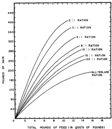
additional, gain equations may be derived from the total-gain equations by taking the first derivative of gain (G) with respect to total feed ('Y).l7 The marg-inal-gain equation is used to estimate the additional gain from the last pound of feed fed of a given ration. Total- and marginal-gain equations, for eight select-ed rations, are derivselect-ed from over-all stilbesh'ol produc-tion funcproduc-tion 8 and are shown in table 10. Similar equations derived from over-all nonstilbestrol produc-tion funcproduc-tion 9 are shown in table 11.
The predicted total-gain values for various levels of feed input for the eight selected rations, are shown in table 12 and plotted in fig. 3 for beef steers fed stil-bestrol. The estimated marginal gain values corre-sponding to the total-gain values are presented in table 13. Similarly, the predicted total-gain values for steers that were not fed stilbestrol are shown in table 14 and plotted in fig. 4, and the associated marginal gains are shown in table 15. The predicted values in both tables 12 and 13 show that, from the same total pounds of feed, total gain and marginal gain monotonically in-crease as the proportion of corn in the ration inin-creases. In table 12, 7,000 pounds of feed of an all-soilage ration is predicted to produce 125.6 pounds of gain; whereas, if the ration is 20:1, the 7,000 pounds of feed will produce 159.6 pounds of beef gains. Other columns in table 12 are interpreted in the same man-ner. Table 13 shows that with 7,000 pounds of all soil-age ration, the marginal gain is 0.0127; with 7,000 pounds of the 20:1 ration, the marginal gain is 0.0180. 11 For the method used, See: Earl O. Heady and John L. Dillon. Agricultllml production functions. Iowa State University Press, Ames, Iowa. 1961.
Table 10. Total and marginal gain equations, derived from the over-all stilbestrol quadratic function, for selected rations for 8S0-pound good-to-chaice feeder
steers.-Prediction equations for:
Ration b Total gain Marginal gain
Ration A GA - 0.023160514 'YA - 0.000000745 'Y"A oG
All soilage - 1.223605 H
o'Y:
=
0.023160514 - 0.000001508 'YARation B GD
=
0.02759913 'YD - 0.000000686 'Y"D oGB20:1 1.223605 H "'YD
=
0.02759913 - 0.000001372 'YDRation C Go
=
0.02898620 'YO - 0.000000672 'Y'o ~Go=
0.0289862015:1 1.223605 H v'YO - 0.000001344 yo
Ration D GD
=
0.0316342899 'YD - 0.000000554 'Y'D aGD10:1 - 1.223605 H a'YD = 0.0316342399 - 0.000001308 'YD
Ration E GE = 0.0335172901 'YE - 0.000000647 'Y"E aG"
8:1 - 1.223605 H a~= 0.0885172901 - 0.000001294 'YE
Ration F GF
=
0.0386956787 'YF - 0.000000651 'Y'F aGF5:1 - 1.223605 H a'YF
=
0.0386956787 - 0.000001802 'YFRation G Go = 0.0484632605 ')'G - 0.000000724 'Y"o aGo
3:1 - 1.223605 H a'Yo = 0.0464682605 - 0.000001448 'YO
Ration H Gu = 0.0542308423 'YII - 0.000000878 'Y'II aGIl
2:1 - 1.223605 H a'YII
=
0.0542308428 - 0.000001756 'YBa In each equation, 'Y denotes total pounds of feed of the particular ration indicated by the small capital letter following 'Y. b Ration is the ratio of soilage to com.
Table 11. Total and marginal gain equations, derived from the over-aU nonstilbestral quadratic function, for selected rations for 8S0-pound good-to-choice feeder steers.o
Prediction equations for:
Rationb Total gain Marginal gain
Ration A
All soilage Ration B
GA - 0.021287744 'YA - 0.000000578 'Y'A
- 2.2005042 H a'YA = 0.021287744 - 0.00000H56 'YA aGA
20:1
Gn = 0.02740.'34765 'Yll - 0.000000724 'Y'B
- 2.2005042 H a'YB aGB = 0.0274034765 - 0.000001448 'YB
Ration C 15:1
Go = 0.0293146425 'YO - 0.000000777 'Y"c
- 2.2005042 H aGe = 0.0293146425 - 0.000001556 'YO a'Yo
Ration D
10:1
GD = 0.0829632826 'YD - 0.000000892 'Y'D
- 2.2005042 H aGD a,),D
=
0.0329632326 - 0.000001784 'YDRation E
8:1
GE = 0.0355577856 'YE - 0.000000982 'Y"!)
- 2.2005042 H ~G" = 0.0355577856 - 0.000001964 'Y"
"'YE
Ration F GF
=
0.0426928071 'YF - 0.000001268 'Y'F aGF = 0.0426928071 _ 0.000002586 'YF5:1 - 2.2005042 H a'YF
Ration G Go = 0.0533953380 'YO - 0.000001802 'Y"o aGo = 0.0533953380 _ 0.000003604 'YG
3:1 - 2.2005042 H a'YG
Ration H Gil = 0.0640978689 'YII - 0.000002461 'Y"II ~= 0.0640978689 _ 0.000004922 'YB
2: 1 - 2.2005042 H O'YII
b In each equation, 'Y denotes total pounds of feed of the particular ration indicated by the small cavital letter following 1'. b Ration is the ratio of soilage to com.
Table 12. Estimated totol gain fram various total feed quantities' ('Y) selected stilbestrol rations fed to 8S0-paund gaod-to-choice feeder steers. &
Pounds Total gaine in pounds for selected ratioDs:d
of feed All fed soilage 20:1 15:1 10:1 8:1 5:1 3:1 2:1 500 11.4 13.6 14.3 15.7 16.6 19.2 23.1 26.9 1,000 22.4 26.9 28.3 31.0 32.9 38.0 45.7 53.4(0) 2,000 _ _ 'ic43~':;;.3 _ _ _ ----:5~2~.5;-_ _ _ ....,53:5",.3<-_ _ _ ~6:;;.0.:;;7 _ _ _ _ 6;;-4~.4.;-_ _ _ .-;7"'4;:;.8;---' 90.0 104.9 3,000 62.8 76.6 80.9 89.0 94.7 110.2 _....:;1;;:;3~2.~9:__--"if.154.8(r) 4,000 80.7 99.4 105.2 116.1 123.7 144.4 174.8 202.9 5,000 97.2 120.9 128.1 141.8 151.4 177.2 214.2 249.2(K) 6,000 H2.1 140.9 149.7 166.3 ,_""""""'1~7"'7~.8;---~2~0~8.';';7---'·1 252.7 298.8 7,000 125.6 159.6 170.0 189.4 202.9 239.0 289.7 336.6(b) 8,000 137.6 176.9 188.8 211.2 226.7 ;--...;2"'6~7="'.9:_--...;;3"'2"'S.'"i:8;__-1 377.7 ( I) 9,000 148.1 192.8 ;--_""20~6;=..4~---:2~3;;;1;:;.7~--~2~49.3 I 295.5 359.5 I 417.0 10,000 _...;;1;.;:5c77.~1,.__----;:2.;:,07"'.4_=_----' 222.6 250.9 270-.5-- 321.8 392.2 454.5 11,000 164.6 220.6 287.5 268.8 1--290~"'.4;---::;3~46"".9;,---' 428.4 12,000 170.6 282.4 251.0 285.4 309.0 870.6 13,000 175.1 242.9 263.2 300.7 14,000 178.1 15,000 179.7
• In addition to the feed fed of selected rations there would also be fed a certain amount of the supplement shown in table 3. This supplement would be fed at the rate of 0.2 of a ponnd per day. The estimated number of feeding days for each of the feed quantities Is shown in table 30.
b Temperature is held constant at the over-all mean • • All valnes are derived from the equations in table 10.
d The ratioll is the ratio of soilage to com, and the letters in parentheses in the last column refer to the feeding periods as follows (see table 29):
e=80 days, f=60 days, g=90 days, h=120 days and ;=140 days, for all quantities above the horizontal line.
Table 13. Estimated marginal gain from various total feed quantities (-yl of selected soilage-corn ration fed to SSO-pound good-to-choice feeder steers {with stilbestroll.
Mnrginal gain" in pounds for selected rations,-Pounds of feed fed 500 1,000 2,000 3,000 4,000 5,000 6,000 7,000 8,000 9,000 10,000 II,OOO 12,000 13,000 14,000 15,000 All soilage 0.0224 0.0217 0.0202 0.0187 0.0171 0.0157 0.0142 0.0127 0.0112 0.0097 0.0083 0.0068 0.0053 0.0038 0.0023 0.0008 20,1 15,1 0.0269 0.0283 0.0262 0.0276 0.0249 0.0263 0.0235 0.0250 0.0221 0.0236 0.0207 0.0223 0.0194 0.0209 0.0180 0.0196 0.0166 0.0182 0.0153 0.0169 0.0139 0.0155 0.0125 0.0142 0.0111 0.0128 0.0098 0.OIl5
• All values have been derived from the equations in table 10.
h The ration is the ratio· of soilage to com.
10,1 8,1 5,1 0.0310 0.0329 0.0380 0.0303 0.0322 0.0374 0.0290 0.0309 0.0361 0.0277 0.0296 0.0348 0.0264 0.0283 0.0335 0.0251 0.0270 0.0322 0.0238 0.0258 0.0309 0.0225 0.0245 0.0296 0.0212 0.0232 0.0283 0.0199 0.0219 0.0270 0.0185 0.0206 0.0257 0.0172 0.0193 0.0244 0.0159 0.0180 0.0230 0.0146 3,1 2,1 0.0457 0.0534 0.0450 0.0525 0.0436 0.0507 0.0421 0.0490 0.0407 0.0472 0.0392 0.0455 0.0378 0.0437 0.0363 0.0419 0.0349 0.0402 0.0334 0.0384 0.0320 0.0367 0.0305
Table 14. Estimated total gain from various total feed quantities' (-yl of selected soilage-corn rations fed to SSO-pound
good-to-choice feeder steers (without stilbestral).· Pounds of feed fed 500 1,000 2,000 3,000 4,000 5,000 6,000 7,000 8,000 9,000 10,000 11,000 12,000 13.000 14,000 15,000 16,000 17,000 All soilage 10.5 20.7 40.3 58.7 75.9 92.0 106.9 120.7 133.3 144.8 155.1 164.3 172.3 179.1 184.8 189.4 192.8 195.0 20,1 13.5 26.7 51.9 75.7 98.0 118.9 138.4 156.4 172.9 188.0 201.7 213.9 224.6 234.0 241.8 248.2
Total gain- in pounds
15,1 10,1 14.5 16.3 28.5 32.1 55.5 62.4 80.9 90.9 104.8 117.6 127.1 142.5 147.9 165.7 167.1 187.0 184.7 206.6 200.8 224.4 215.4 240.4 228.4 254.7 239.8 267.1 249.7 277.8 258.0 286.7 264.8
for selected rations, 4
8,1 5,1 3,1 2:1 17.5 21.0 26.2 31.4 34.6 41.4 51.6 61.6(0) 67.2 80.3 99.6 II8.4 97.8 116.7 144.0 170.1(') 126.5 150.5 184.8 217.0 153.2 181.8 221.9 259.0(K) 178.0 210.5 255.5 296.0 200.8 236.7 285.5 328.1(h) 221.6 260.4 311.8 355.3(1 ) 240.5 281.5 334.6 377.5 257.4 300.1 353.8 394.8 272.3 316.2 369.3 285.3 329.7 296.3 305.3
• In addition to the feed fed. there would also be fed a certain amount of the supplement shown in table 3. This supplement would be fed at the' rate of 0.2 of a pound per day. The estimated number of feeding days for each of the feed quantities is shown in table 31.
b Temperature is held constant at the over-all mean.
e All values are derived from the equations in table 11.
d The ration is the ratio of soilage to com. The letters in parentheses above (,Rch horizonlal line refer to the feeding periods: e=:30 days, f=60 days, g=90 days, h=120 days and i=over 120 days and up to 140 days for quantities below the line, traced out by the horizontal lines.
Table 15. Estimated marginal gain from various totol feed quantities (-y) of selected soilage-corn ration fed to SSO-pound
good-to-choice feeder steers (without stilbestrol).
Marginal gain' in pounds for selected rations: b
Pound. of feed All fed soilage 500 0.0207 1,000 0.0201 2,000 0.0190 3,000 0.0178 4,000 0.0167 5,000 0.0155 6,000 0.0144 7,000 0.0132 8,000 0.0120 9,000 0.0109 10,000 0.0097 11,000 0.00'16 12,000 0.0074 13,000 0.0063 14,000 0.0051 15,000 0 0040 16,000 0.0028 17.000 0.0017 20:1 0.0267 0.0260 0.0245 0.0231 0.0216 0.0202 0.0187 0.0173 0.0158 0.0144 0.0129 0.0115 0.0100 0.0086 0.0071 0.0057 15:1 0.0~88 0.0278 0.0262 0.0246 00231 0.0215 00'200 0.0184 0.0169 0.0153 0.0138 0.0122 0.0107 0.0091 0.0075 0.0060 • All values have been derived from the equations in table 11.
h The ration is the ratio of soilage to com.
10:1 001121 0.0312 0.0294 0.0276 0.0258 0.0240 0.0223 0.0205 00187 0.0169 0.0151 0.0133 0.0116 0.0097 0.0080 8:1 0.0346 0.0336 0.0316 0.09.97 0.0277 0.0257 0.0238 0.0218 0.0198 0.0179 0.0159 0.0140 0.0120 0.0100 0.0081 5:1 0.0414 0.0402 0.0376 0.0351 0.0325 0.0300 0.0275 0.0249 0.0224 0.0199 0.0173 0.0148 0.0122 3:1 0.0516 0.0498 0.0462 0.0426 0.0390 0.0354 0.0318 0.0282 0.0246 0.0210 0.0174 0.0138 2:1 0.0616 0.0592 0.0543 0.0493 0.0444 0.0395 0.0346 0.0296 0.0247 0.0198 0.0149